A measure of betweenness centrality
based on random walks

Abstract

Betweenness is a measure of the centrality of a node in a network, and is normally calculated as the fraction of shortest paths between node pairs that pass through the node of interest. Betweenness is, in some sense, a measure of the influence a node has over the spread of information through the network. By counting only shortest paths, however, the conventional definition implicitly assumes that information spreads only along those shortest paths. Here we propose a betweenness measure that relaxes this assumption, including contributions from essentially all paths between nodes, not just the shortest, although it still gives more weight to short paths. The measure is based on random walks, counting how often a node is traversed by a random walk between two other nodes. We show how our measure can be calculated using matrix methods, and give some examples of its application to particular networks.

1 Introduction

Over the years network researchers have introduced a large number of centrality indices, measures of the varying importance of the vertices in a network according to one criterion or another (Wasserman and Faust 1994; Scott 2000). These indices have proved of great value in the analysis and understanding of the roles played by actors in social networks, as well as by vertices in networks of other types, including citation networks, computer networks, and biological networks. Perhaps the simplest centrality measure is degree, which is the number of edges incident on a vertex in a network—the number of ties an actor has in social network parlance. Degree is a measure in some sense of the popularity of an actor. A more sophisticated centrality measure is closeness, which is the mean geodesic (i.e., shortest-path) distance between a vertex and all other vertices reachable from it. Closeness can be regarded as a measure of how long it will take information to spread from a given vertex to others in the network.

Another important class of centrality measures is the class of betweenness measures. Betweenness, as one might guess, is a measure of the extent to which a vertex lies on the paths between others. The simplest and most widely used betweenness measure is that of Freeman (1977; 1979), usually called simply betweenness. (Where necessary, to distinguish this measure from other betweenness measures considered in this paper, we will refer to it as shortest-path betweenness.) The betweenness of a vertex $i$ is defined to be the fraction of shortest paths between pairs of vertices in a network that pass through $i$. If, as is frequently the case, there is more than one shortest path between a given pair of vertices, then each such path is given equal weight such that the weights sum to unity. To be precise, suppose that $g^{(st)}_{i}$ is the number of geodesic paths from vertex $s$ to vertex $t$ that pass through $i$, and suppose that $n_{st}$ is the total number of geodesic paths from $s$ to $t$. Then the betweenness of vertex $i$ is

$$b_{i}={\sum_{s<t}g^{(st)}_{i}/n_{st}\over\frac{1}{2}n(n-1)},$$ (1)

where $n$ is the total number of vertices in the network. We may, or may not, according to taste, consider the end-points of a path to fall on that path; the choice makes only the difference of an additive constant in the values for $b_{i}$. In this paper we will generally include the end-points.

Betweenness centrality can be regarded as a measure of the extent to which an actor has control over information flowing between others. In a network in which flow is entirely or at least mostly along geodesic paths, the betweenness of a vertex measures how much flow will pass through that particular vertex. Betweenness can be calculated for all vertices in time $\mathrm{O}(mn)$ for a network with $m$ edges and $n$ vertices (Newman 2001; Brandes 2001).

In most networks however, information (or anything else) does not flow only along geodesic paths (Stephenson and Zelen 1989; Freeman et al. 1991). News or a rumor or a message or a fad does not know the ideal route to take to get from one place to another; more likely it wanders around more randomly, encountering who it will. And even in a case such as the famous small-world experiment of Milgram (1967; Travers and Milgram 1969), or its modern-day equivalent (Dodds et al. 2003), in which participants are explicitly instructed to get a message to a target by the most direct route possible, there is no evidence that people are especially successful in this task. Thus we would imagine that in most cases a realistic betweenness measure should include non-geodesic paths in addition to geodesic ones.

Furthermore, by giving all the weight to the geodesic paths, and none to any other paths, no matter how closely competitive they are, the shortest-path betweenness measure can produce some odd effects. Consider the network sketched in Fig. 1a, for instance, in which two large groups are bridged by connections among just a few of their members. Vertices A and B will certainly get high betweenness scores in this case, since all shortest paths between the two communities must pass through them. Vertex C on the other will hand get a low score, since none of those shortest paths pass through it, taking instead the direct route from A to B. It is plausible however that in many real-world situations C would have quite a significant role to play in information flows. Certainly it is possible for information to flow between two individuals via a third mutual acquaintance, even when the two individuals in question are themselves well acquainted.

Figure 1: (a) Vertices A and B will have high (shortest-path) betweenness in this configuration, while vertex C will not. (b) In calculations of flow betweenness, vertices A and B in this configuration will get high scores while vertex C will not.

To address these problems, Freeman et al. (1991) suggested a more sophisticated betweenness measure, usually known as flow betweenness, that includes contributions from some non-geodesic paths. Flow betweenness is based on the idea of maximum flow. Imagine each edge in a network as a pipe that can carry a unit flow of some fluid. We can ask what the maximum possible flow then is between a given source vertex $s$ and target vertex $t$ through these pipes. In general the answer is that more than a single unit of flow can be carried between source and target by making simultaneous use of several different paths through the network. The flow betweenness of a vertex $i$ is defined as the amount of flow through vertex $i$ when the maximum flow is transmitted from $s$ to $t$, averaged over all $s$ and $t$. Maximum flow from a given $s$ to all reachable targets $t$ can be calculated in worst-case time $\mathrm{O}(m^{2})$ using, for instance, the augmenting path algorithm (Ahuja et al. 1993), and hence the flow betweenness for all vertices can be calculated in time $\mathrm{O}(m^{2}n)$.

In practical terms, one can think of flow betweenness as measuring the betweenness of vertices in a network in which a maximal amount of information is continuously pumped between all sources and targets. Necessarily, that information still needs to “know” the ideal route (or one of the ideal routes) from each source to each target, in order to realize the maximum flow. Although the flow betweenness does take account of paths other than the shortest path (and indeed need not take account of the shortest path at all), this still seems an unrealistic definition for many practical situations: flow betweenness suffers from some of the same drawbacks as shortest-path betweenness, in that it is often the case that flow does not take any sort of ideal path from source to target, be it the shortest path, the maximum flow path, or another kind of ideal path.

Moreover, like the shortest-path measure, flow betweenness can give counterintuitive results in some cases. Consider for example the network sketched in Fig. 1b, which again has two large groups joined by a few contacts. In this case, the maximum flow from one group to the other is clearly limited to two units, one unit flowing through each of vertices A and B. Vertex C will, in this case, get a low betweenness score, even though the path through C may be as short or shorter than that through A or B. Once again, it is plausible that in practical situations C would actually play quite a significant role.

In this paper, therefore, we propose a new betweenness measure, which might be called random-walk betweenness. Roughly speaking, the random-walk betweenness of a vertex $i$ is equal to the number of times that a random walk starting at $s$ and ending at $t$ passes through $i$ along the way, averaged over all $s$ and $t$. This measure is appropriate to a network in which information wanders about essentially at random until it finds its target, and it includes contributions from many paths that are not optimal in any sense, although shorter paths still tend to count for more than longer ones since it is unlikely that a random walk becomes very long without finding the target. In some sense, our random-walk betweenness and the shortest-path betweenness of Freeman (1977) are at opposite ends of a spectrum of possibilities, one end representing information that has no idea of where it is going and the other information that knows precisely where it is going. Some real-world situations may mimic these extremes while others, such as perhaps the small-world experiment, fall somewhere in between. In the latter case it may be of use to compare the predictions of the two measures to see how and by how much they differ: if they differ little, then either is a reasonable metric by which to characterize the system; if they differ by a lot, then we may need to know more about the particular mode of information propagation in the network to make meaningful judgments about betweenness of vertices.

Our random-walk betweenness can, as we will show, be calculated for all vertices in a network in worst-case time $\mathrm{O}((m+n)n^{2})$ using matrix methods, making it comparable in its computational demands with flow betweenness.

Some other centrality measures based on random walks merit a mention in this context, although none of them are betweenness measures. Bonacich’s power centrality (Bonacich 1987) can be derived in a number of ways, but one way of looking at it is in terms of random walks that have a fixed probability $\beta$ of dying per step. The power centrality of vertex $i$ is the expected number of times such a walk passes through $i$, averaged over all possible starting points for the walk. The random-walk centrality introduced recently by Noh and Rieger (2003) is a measure of the speed with which randomly walking messages reach a vertex from elsewhere in the network—a sort of random-walk version of closeness centrality. The information centrality of Stephenson and Zelen (1989) is another closeness measure, which bears some similarity to that of Noh and Rieger. In essence it measures the harmonic mean length of paths ending at a vertex $i$, which is smaller if $i$ has many short paths connecting it to other vertices.

The outline of this paper is as follows. In Sec. 2 we define in detail our random-walk betweenness and show how it is calculated. We introduce the measure first using an analogy to the flow of electrical current in a circuit, and then show that this is equivalent also to the flow of a random walk. In Sec. 3 we give a number of examples of applications of our measure, first to networks artificially designed to pose a challenge for the calculation of betweenness, and then to various real-world social networks, including a collaboration network of scientists, a network of sexual contacts, and Pagdett’s network of intermarriages between prominent families in 15th century Florence. In Sec. 4 we give our conclusions.

2 Random-walk betweenness

In this section we give the definition of our random-walk betweenness measure and derive matrix expressions that allow it to be calculated rapidly using a computer. For pedagogical purposes, we will take a slightly circuitous route in developing our ideas. We start by introducing a definition of our betweenness measure that does not use random walks but instead is based on current flow in electrical circuits. This definition is simple and intuitive and makes for easy calculations. Later we introduce the random-walk definition of our measure and prove that the two definitions are the same. The developments of this section follow similar lines to a previous presentation we have given on methods for hierarchical clustering (Newman and Girvan 2003).

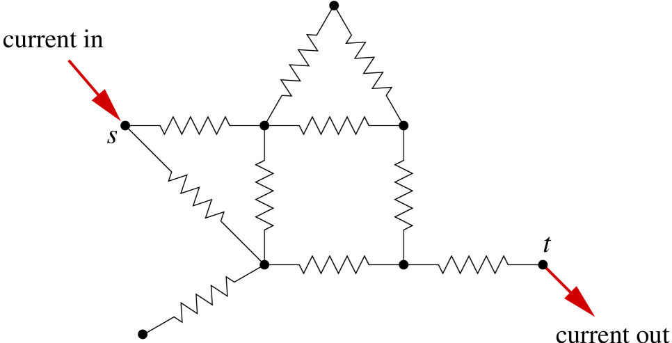
Figure 2: An electrical circuit as discussed in the text, in which the edges of a network have been replaced by identical unit resistors, and unit current is injected at vertex $s$ and removed at vertex $t$. The betweenness of a vertex is defined to be equal to the current flowing through that vertex averaged over all $s$ and $t$.

2.1 A current flow analogy

Consider, then, an electrical circuit created by placing a unit resistance on every edge of the network of interest, as shown in Fig. 2. One unit of current is injected into the network at a source vertex $s$ and one unit extracted at a target vertex $t$, so that current in the network as a whole is conserved. We now define the current-flow betweenness of a vertex $i$ to be the amount of current that flows through $i$ in this setup, averaged over all $s$ and $t$.

Let $V_{i}$ be the voltage at vertex $i$ in the network, measured relative to any convenient point. Kirchhoff’s law of current conservation states that the total current flow into or out of any vertex is zero, which implies that the voltages satisfy the equations

$$\sum_{j}A_{ij}(V_{i}-V_{j})=\delta_{is}-\delta_{it},$$ (2)

for all $i$, where $A_{ij}$ is an element of the adjacency matrix thus:

$$A_{ij}=\biggl{\{}\begin{array}[]{rl}1&\qquad\mbox{if there is an edge between $i$ and $j$,}\\ 0&\qquad\mbox{otherwise,}\end{array}$$ (3)

and $\delta_{ij}$ is the Kronecker $\delta$:

$$\delta_{ij}=\biggl{\{}\begin{array}[]{rl}1&\qquad\mbox{if $i=j$,}\\ 0&\qquad\mbox{otherwise.}\end{array}$$ (4)

Noting that $\sum_{j}A_{ij}=k_{i}$, the degree of vertex $i$, we can write Eq. (2) in matrix form as

$$(\mathbf{D}-\mathbf{A})\cdot\mathbf{V}=\mathbf{s},$$ (5)

where $\mathbf{D}$ is the diagonal matrix with elements $D_{ii}=k_{i}$ and the source vector $\mathbf{s}$ has elements

$$s_{i}=\Biggl{\{}\begin{array}[]{rl}+1&\qquad\mbox{for $i=s$,}\\ -1&\qquad\mbox{for $i=t$,}\\ 0&\qquad\mbox{otherwise.}\end{array}$$ (6)

We cannot simply invert the matrix $\mathbf{D}-\mathbf{A}$ to get the voltage vector $\mathbf{V}$, because the matrix (which is called the graph Laplacian) is singular: the vector $\mathbf{V}=(1,1,1,\ldots)$ is always an eigenvector with eigenvalue zero because voltage is arbitrary to within an additive constant, and since the determinant is the product of the eigenvalues, it follows that the determinant is always zero. Mathematically, this says that one of the equations in our system of $n$ equations is redundant. (Physically, it is telling us that current is conserved.) To fix the problem we need only choose one equation, any equation, and remove it from the system, to get a matrix we can invert. This operation is made most simple if we simultaneously choose to measure our voltages relative to the corresponding vertex. Thus, let us measure voltages relative to some vertex $v$, and remove the $v$th equation, which means removing the $v$th row of $\mathbf{D}-\mathbf{A}$. Since $V_{v}=0$, we can also remove the $v$th column, giving a square $(n-1)\times(n-1)$ matrix, which we denote $\mathbf{D}_{v}-\mathbf{A}_{v}$. Then

$$\mathbf{V}=(\mathbf{D}_{v}-\mathbf{A}_{v})^{-1}\cdot\mathbf{s}.$$ (7)

The voltage of the one missing vertex $v$ is, by definition, zero. To represent this, let us now add a $v$th row and column back into $(\mathbf{D}_{v}-\mathbf{A}_{v})^{-1}$ with values all equal to zero. The resulting matrix we will denote $\mathbf{T}$. Then, using Eq. (6), the voltage at vertex $i$ for source $s$ and target $t$ is given in terms of the elements of $\mathbf{T}$ by

$$V^{(st)}_{i}=T_{is}-T_{it}.$$ (8)

The current flowing through the $i$th vertex is given by a half of the sum of the absolute values of the currents flowing along the edges incident on that vertex:

$$I^{(st)}_{i}=\mbox{$\frac{1}{2}$}\sum_{j}A_{ij}|V^{(st)}_{i}-V^{(st)}_{j}|=\mbox{$\frac{1}{2}$}\sum_{j}A_{ij}|T_{is}-T_{it}-T_{js}+T_{jt}|,\quad\mbox{for $i\neq s,t$.}$$ (9)

As noted, this expression does not work for the source and target vertices, for which one also has to take account of the current injected and removed from the network, but these vertices necessarily have a current flow of exactly one unit, so one can simply write

$$I^{(st)}_{s}=1,\qquad I^{(st)}_{t}=1.$$ (10)

(Alternatively, if one is adopting the convention under which the end-points of a path are not considered part of that path, then one should set these two currents to 0 rather than 1.) Then the betweenness is the average of the current flow over all source-target pairs:

$$b_{i}={\sum_{s<t}I^{(st)}_{i}\over\frac{1}{2}n(n-1)}.$$ (11)

If the network has more than one component, then the procedure described here should be repeated separately for each component.

The inversion of the matrix takes time $\mathrm{O}(n^{3})$, while the evaluation of Eq. (11) takes time $\mathrm{O}(mn)$ for each vertex or $\mathrm{O}(mn^{2})$ for all of them. Thus the total running time to calculate the current-flow betweenness for all vertices is $\mathrm{O}((m+n)n^{2})$, or $\mathrm{O}(n^{3})$ on a sparse graph. This is comparable with the time for calculation of the flow betweenness, although slower than the fastest algorithms for shortest-path betweenness. In our experience, the calculation is tractable for networks up to about $10\,000$ vertices using typical desktop computing resources available at the time of writing.

This current-flow betweenness measure seems an intuitively reasonable one. Current will flow along all paths from source to target, but more along shorter than longer ones, the shorter ones offering less resistance than the longer. And vertices that lie on no path from source to target, those that sit in a cul-de-sac off to the side of the network, get a betweenness of zero, which is also sensible. However, there is no special reason to believe that the flow of electrical current has anything to do with processes in non-electrical networks, such as social networks. In the following section, therefore, we introduce our random-walk betweenness, whose definition, we believe, is relevant for social networks and other types of networks also, and we show that it is in fact numerically equal to the current-flow betweenness.

2.2 Random walks

Imagine a “message,” which could be information of almost any kind, that originates at a source vertex $s$ on a network. The message is intended for some target $t$, but the message, or those passing it, have no idea where $t$ is, so the message simply gets passed around at random until it finds itself at $t$. Thus, on each step of its travels, the message moves from its current position on the network to one of the adjacent vertices, chosen uniformly at random from the possibilities. This is a random walk.

With the important proviso discussed in the following paragraph, let us define a betweenness measure for a vertex $i$ that is equal to the number of times that the message passes through $i$ on its journey, averaged over a large number of trials of the random walk. The full random-walk betweenness of vertex $i$ will then be this value averaged over all possible source/target pairs $s,t$.

There is one small, but important, further technical point. It would be perfectly possible for a vertex to accrue a high betweenness score if a random walk were simply to walk back and forth through that vertex many times, without actually going anywhere. This situation does not correspond to our intuition of what it means to have high betweenness, and indeed if we count walks in this way our betweenness measure is found to give mostly useless results. So instead, we define the betweenness of vertex $i$ to be the net number of times a walk passes through $i$. By “net” we mean that if a walk passes through a vertex and then later passes back through it in the opposite direction, the two cancel out and there is no contribution to the betweenness. Furthermore, if, when averaged over many possible realizations of the walk in question, we find that the walk is equally likely to pass in either direction through a vertex, then again the two directions cancel. How we allow for these cancellations in practice will become clear shortly.

Consider then an absorbing random walk, a walk that starts at vertex $s$ and makes random moves around the network until it finds itself at vertex $t$ and then stops. If at some point in this walk we find ourselves at vertex $j$, then the probability that we will find ourselves at $i$ on the next step is given by the matrix element

$$M_{ij}={A_{ij}\over k_{j}},\qquad\mbox{for $j\neq t$,}$$ (12)

where once again $A_{ij}$ is an element of the adjacency matrix, Eq. (3), and $k_{j}=\sum_{i}A_{ij}$ is the degree of vertex $j$. In matrix notation, we can write $\mathbf{M}=\mathbf{A}\cdot\mathbf{D}^{-1}$, where $\mathbf{D}$ is, as before, the diagonal matrix with elements $D_{ii}=k_{i}$.

The only exception to Eq. (12), as noted, is for $j=t$; since this is an absorbing random walk, we never leave $t$ once we get there (a behavior sometimes jokingly called the “Hotel California effect”), so $M_{it}=0$ for all $i$. Alternatively, we can simply remove row $t$ from the matrix altogether. We can also remove column $t$ without affecting transitions between any other vertices. Let us denote by $\mathbf{M}_{t}=\mathbf{A}_{t}\cdot\mathbf{D}_{t}^{-1}$ the matrix with these elements removed, and similarly for $\mathbf{A}_{t}$ and $\mathbf{D}_{t}$.

Now for a walk starting at $s$, the probability that we find ourselves at vertex $j$ after $r$ steps is given by $[\mathbf{M}_{t}^{r}]_{js}$, and the probability that we then take a step to an adjacent vertex $i$ is $k_{j}^{-1}[\mathbf{M}_{t}^{r}]_{js}$. Summing over all values of $r$ from 0 to $\infty$, the total number of times we go from $j$ to $i$, averaged over all possible walks, is $k_{j}^{-1}[(\mathbf{I}-\mathbf{M}_{t})^{-1}]_{js}$. In matrix notation we can write this as an element of the vector

$$\mathbf{V}=\mathbf{D}_{t}^{-1}\cdot(\mathbf{I}-\mathbf{M}_{t})^{-1}\cdot\mathbf{s}=(\mathbf{D}_{t}-\mathbf{A}_{t})^{-1}\cdot\mathbf{s},$$ (13)

where $\mathbf{s}$ is defined as before—see Eq. (6). (The element $s_{t}=-1$ is not strictly necessary—we could give $s_{t}$ any value we like, since row $t$ is removed from the equations anyway. We make this particular choice in order to demonstrate that our random-walk betweenness is the same as the current-flow betweenness.) Clearly this equation is precisely the same as Eq. (7), for the particular choice $v=t$.

Now the net flow of the random walk along the edge from $j$ to $i$ is given by the absolute difference $|V_{i}-V_{j}|$ and the net flow through vertex $i$ is a half the sum of the flows on the incident edges, just as in Eq. (9). The rest of the derivation follows through as before, and the final net flow of random walks through vertex $i$ is given by Eq. (11). (Although Eq. (13) was derived for the particular case in which the $t$th row and column are removed from the matrix $\mathbf{D}-\mathbf{A}$, the developments of Sec. 2.1 show that the same result can be derived by removing any row and column.)

To summarize, the prescription for calculating random-walk betweenness, which is the expected net number of times a random walk passes through vertex $i$ on its way from a source $s$ to a target $t$, averaged over all $s$ and $t$, is as follows for each separate component of the graph of interest.

1. Construct the matrix $\mathbf{D}-\mathbf{A}$, where $\mathbf{D}$ is the diagonal matrix of vertex degrees and $\mathbf{A}$ is the adjacency matrix.

2. Remove any single row, and the corresponding column. For example, one could remove the last row and column.

3. Invert the resulting matrix and then add back in a new row and column consisting of all zeros in the position from which the row and column were previously removed (e.g., the last row and column). Call the resulting matrix $\mathbf{T}$, with elements $T_{ij}$.

4. Calculate the betweenness from Eq. (11), using the values of $I_{i}$ from Eqs. (9) and (10).

3 Examples and applications

In this section we give a number of examples to illustrate the properties and use of our random-walk betweenness measure in the analysis of network data.

3.1 Simple examples

We start off by presenting some cases with which previous betweenness measures have difficulties, but for which, as we now show, our new measure works well. Our examples are based on the graphs sketched in Fig. 1, with the two groups consisting of complete graphs of five vertices each, as depicted in Fig. 3. We show figures for the betweenness scores in Table 1.

Figure 3: Example networks of the types sketched in Fig. 1, with the groups represented by completely connected graphs of five vertices each.

		betweenness measure
network		shortest-path	flow	random-walk
Network 1:	vertices A & B	$0.636$	$0.631$	$0.670$
	vertex C	$0.200$	$0.282$	$0.333$
	vertices X & Y	$0.200$	$0.068$	$0.269$
Network 2:	vertices A & B	$0.265$	$0.269$	$0.321$
	vertex C	$0.243$	$0.004$	$0.267$
	vertices X & Y	$0.125$	$0.024$	$0.194$

Table 1: Betweenness values calculated using shortest-path, flow, and random-walk measures for the two networks of Fig. 3. In each network, we intuitively expect vertex C to have betweenness lower than that of vertices A and B, but higher than that of vertices X and Y. The shortest-path and flow betweenness measures each fail to do this for one of these two challenging networks (numbers in boxes). Our random-walk measure on the other hand orders the vertices correctly in each case.

As the table shows, the shortest path betweenness fails to give a higher score to vertex C in the first network than to any of the other vertices within the two communities, while flow betweenness has the same problem with vertex C in the second network. In both cases, by contrast, our random-walk betweenness gives vertex C a distinctly higher score, reflecting our intuition that this vertex has a higher centrality in both of the networks.

3.2 Correlation with other measures

Shortest-path betweenness is known to be strongly correlated with vertex degree in most networks (Nakao 1990; Goh et al. 2003), and it has been argued that this makes it a less useful measure. If the two are strongly correlated, then what is the point of going to the effort of calculating betweenness, when degree is almost the same and much easier to calculate? The answer is that there are usually a small number of vertices in a network for which betweenness and degree are very different, and betweenness is useful precisely in identifying these vertices.

Figure 4: Scatter plots of the random-walk betweenness of vertices in the sexual contact network of Fig. 5, against vertex degree (left) and standard shortest-path betweenness (right). The dotted lines indicate the best linear fits in each case, which have the correlation coefficients indicated.

We can look at a similar question for our random-walk measure. In Fig. 4, for example, we show scatter plots of random-walk betweenness vs. (a) degree and (b) shortest-path betweenness for the actors in a network of sexual contacts drawn from the study of Potterat et al. (2002). As the figure shows, the random-walk betweenness is moderately highly correlated with degree ($r^{2}=0.626$) and very highly correlated with shortest-path betweenness ($r^{2}=0.923$). Thus, in general, vertices with higher degree or higher shortest-path betweenness tend also to have higher random-walk betweenness. However, this observation misses the real point of interest, which is that there are a few vertices that have random-walk betweenness values quite different from their scores on the other two measures.

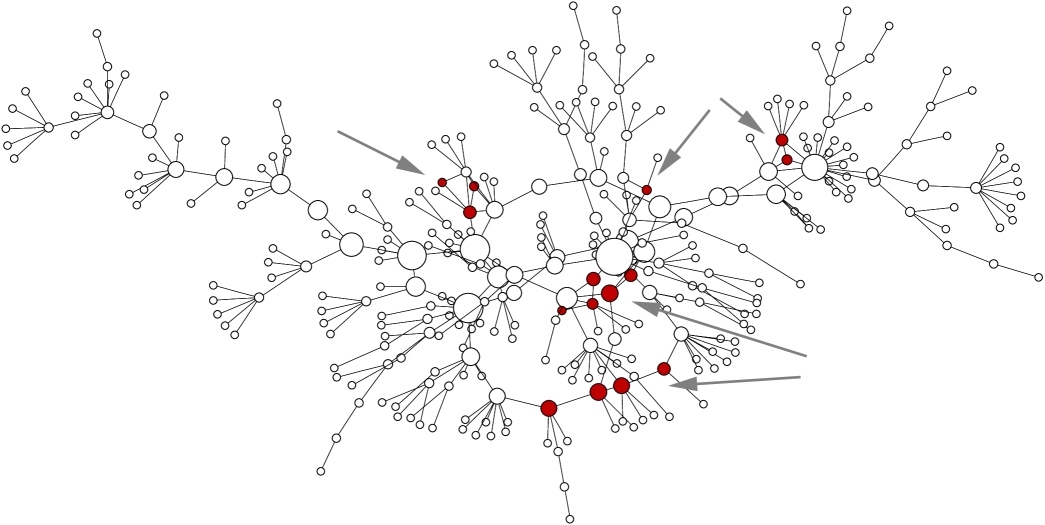
Figure 5: The largest component of a network of sexual contacts between high-risk actors in the city of Colorado Springs, CO, as reconstructed by Potterat et al. (2002). The size of the vertices increases linearly with their random-walk betweenness, as defined in this paper. The highlighted vertices (also indicated by the arrows) are those for which the random-walk betweenness is substantially greater than shortest-path betweenness (a factor of two or more).

In Fig. 5 we show a picture of the network in question, in which we have drawn each the vertices with a size indicating their random-walk betweenness score. It is immediately clear that some, but not all, of the high-degree vertices have high random-walk betweenness. Furthermore, we have highlighted the vertices in the network for which the random-walk betweenness is more than twice their shortest-path betweenness—these are vertices which the shortest-path measure misses because, although they lie on many paths between others, they don’t lie on many shortest paths.

The primary reason for the study of networks of sexual contacts is to improve our understanding of the propagation and control of sexually transmitted diseases. Certainly there is no reason to suppose that diseases always know precisely where they are going and spread along the shortest path to some “target” victim. A random-walk model of disease spread is probably a more reasonable representation of what actually happens, in which case the highlighted nodes in Fig. 5 are nodes that are likely to be responsible for transmission of the disease to others, but which would be missed if we evaluated the centralities using standard shortest-path-based methods.

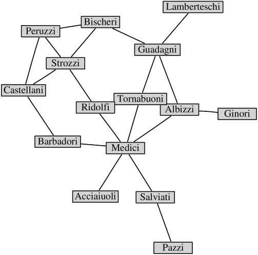
Figure 6: The network of intermarriage relations between the 15th century Florentine families studied by Padgett and Ansell (1993). One family, Pucci, which had no marriage ties with others, is omitted from the picture.

3.3 Example applications

We now give two brief examples of applications of our betweenness measure to previously studied networks. First, we look at Padgett’s famous network of intermarriages between prominent families in early 15th century Florence (Padgett and Ansell 1993), depicted in Fig. 6. In Table 2, we rank the fifteen families by their random-walk betweenness, finding that the Medici come out well ahead of the competition, and in particular, they easily best their arch-rivals, the Strozzi. It is suggested that that it was in part the Medici’s skillful manipulation of this marriage network that led to their eventual dominance of the Florentine political landscape.

family	betweenness	family	betweenness
Medici	$0.652420$	Barbadori	$0.269363$
Guadagni	$0.451309$	Salviati	$0.257143$
Albizzi	$0.362961$	Peruzzi	$0.245624$
Strozzi	$0.333302$	Pazzi	$0.133333$
Ridolfi	$0.317014$	Lamberteschi	$0.133333$
Bischeri	$0.314018$	Ginori	$0.133333$
Tornabuoni	$0.306102$	Acciaiuoli	$0.133333$
Castellani	$0.284705$

Table 2: The random-walk betweenness scores of the fifteen families in the network of Fig. 6.

As a second example, we show in Fig. 7 the largest component of a coauthorship network taken from the study by Newman and Park (2003). The actors in this network are scientists, primarily in applied mathematics and theoretical physics, who work on graph theory and related mathematical studies of networks, and ties represent coauthorship of papers. As in Fig. 5, the size of the vertices represents their betweenness, calculated using our random-walk measure. As we can see there are a number of actors central to the groups in the network who have high betweenness, although there are others who do not. And there are less central actors with high betweenness because they are the brokers who establish connections between different groups (e.g., those labeled “A” in the figure). But notice also that, where there are two (or more) paths to an outlying group of vertices, those along all paths get a high score (e.g., those labeled “B”), since the random-walk betweenness counts all paths and not just geodesic ones.

4 Conclusions

Betweenness is a measure of network centrality that counts the paths between vertex pairs on a network that pass through a given vertex. Vertices with high betweenness lie on paths between many others and may thus have some influence over the spread of information across the network. One can define a variety of different betweenness measures, depending on which paths one counts and how they are weighted. The most widely used measure, first proposed by Freeman (1977), counts only shortest paths, and is thus appropriate to cases in which information flow is entirely or mostly along such paths. Flow betweenness (Freeman et al. 1991) counts all paths that carry information when a maximum flow is pumped between each pair of vertices. In many networks, however, neither of these cases is realistic. Both count only a small subset of possible paths between vertices, and both assume some kind of optimality in information transmission (shortest paths or maximum flow).

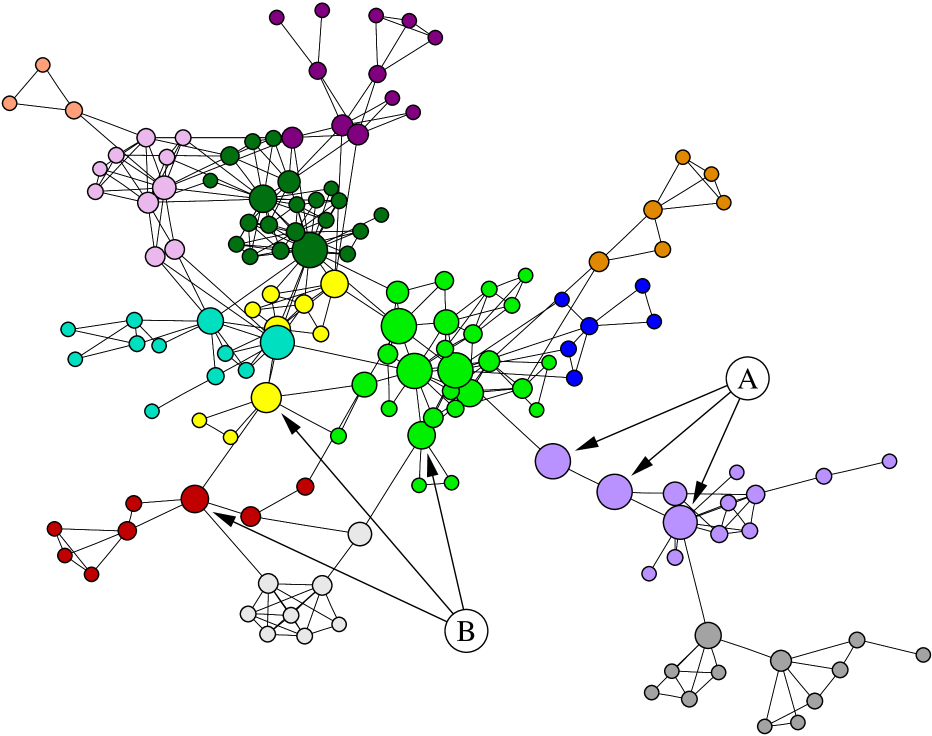
Figure 7: The largest component of the coauthorship network of scientists working on networks from Newman and Park (2003). Size of vertices represents their score on the random-walk betweenness measure developed here. Vertices on a single path from one part of the network to another, such as those labeled “A,” get a high score. So however do those labeled “B,” even though they lie on one of several paths between different parts of the network. The colors of the vertices represent one possible clustering of the network, according to the method of Girvan and Newman (2002), and are included as a guide to the eye.

In this paper we have proposed a new betweenness measure that counts essentially all paths between vertices (we exclude those that don’t actually lead from the designated source to the target), and which makes no assumptions of optimality. Our measure is based on random walks between vertex pairs and asks, in essence, how often a given vertex will fall on a random walk between another pair of vertices. The measure is particularly useful for finding vertices of high centrality that do not happen to lie on geodesic paths or on the paths formed by maximum-flow cut-sets. We have shown that our betweenness can be calculated using matrix inversion methods in time that scales as the cube of the number of vertices on a sparse graph, making it computationally tractable for networks typical of current sociological studies.

We have given a number of brief examples of the use of our betweenness measure, including artificial examples illustrating cases in which it gives substantially different results from previous measures, an example of how it correlates with other measures in a network of sexual contacts, and two applications to previously studied networks, Padgett’s famous Florentine families, and a network of collaborations between scientists. We would be delighted to see more, and more extensive, applications of our random-walk betweenness measure in future studies.

References

- Ahuja et al. (1993) Ahuja, R. K., Magnanti, T. L., and Orlin, J. B., 1993. Network Flows: Theory, Algorithms, and Applications. Prentice Hall, Upper Saddle River, New Jersey.
- Bonacich (1987) Bonacich, P. F., 1987. Power and centrality: A family of measures. Am. J. Sociol. 92, 1170–1182.
- Brandes (2001) Brandes, U., 2001. A faster algorithm for betweenness centrality. Journal of Mathematical Sociology 25, 163–177.
- Dodds et al. (2003) Dodds, P. S., Muhamad, R., and Watts, D. J., 2003. An experimental study of search in global social networks. Science 301, 827–829.
- Freeman (1977) Freeman, L. C., 1977. A set of measures of centrality based upon betweenness. Sociometry 40, 35–41.
- Freeman (1979) Freeman, L. C., 1979. Centrality in social networks: Conceptual clarification. Social Networks 1, 215–239.
- Freeman et al. (1991) Freeman, L. C., Borgatti, S. P., and White, D. R., 1991. Centrality in valued graphs: A measure of betweenness based on network flow. Social Networks 13, 141–154.
- Girvan and Newman (2002) Girvan, M. and Newman, M. E. J., 2002. Community structure in social and biological networks. Proc. Natl. Acad. Sci. USA 99, 7821–7826.
- Goh et al. (2003) Goh, K.-I., Oh, E., Kahng, B., and Kim, D., 2003. Betweenness centrality correlation in social networks. Phys. Rev. E 67, 017101.
- Milgram (1967) Milgram, S., 1967. The small world problem. Psychology Today 2, 60–67.
- Nakao (1990) Nakao, K., 1990. Distribution of measures of centrality: Enumerated distributions of Freeman’s graph centrality measures. Connections 13(3), 10–22.
- Newman (2001) Newman, M. E. J., 2001. Scientific collaboration networks: II. Shortest paths, weighted networks, and centrality. Phys. Rev. E 64, 016132.
- Newman and Girvan (2003) Newman, M. E. J. and Girvan, M., 2003. Finding and evaluating community structure in networks. Preprint cond-mat/0308217.
- Newman and Park (2003) Newman, M. E. J. and Park, J., 2003. Why social networks are different from other types of networks. Preprint cond-mat/0305612.
- Noh and Rieger (2003) Noh, J. D. and Rieger, H., 2003. Random walks on complex networks. Preprint cond-mat/0307719.
- Padgett and Ansell (1993) Padgett, J. F. and Ansell, C. K., 1993. Robust action and the rise of the Medici, 1400–1434. Am. J. Sociol. 98, 1259–1319.
- Potterat et al. (2002) Potterat, J. J., Phillips-Plummer, L., Muth, S. Q., Rothenberg, R. B., Woodhouse, D. E., Maldonado-Long, T. S., Zimmerman, H. P., and Muth, J. B., 2002. Risk network structure in the early epidemic phase of HIV transmission in Colorado Springs. Sexually Transmitted Infections 78, i159–i163.
- Scott (2000) Scott, J., 2000. Social Network Analysis: A Handbook. Sage Publications, London, 2nd ed.
- Stephenson and Zelen (1989) Stephenson, K. A. and Zelen, M., 1989. Rethinking centrality: Methods and examples. Social Networks 11, 1–37.
- Travers and Milgram (1969) Travers, J. and Milgram, S., 1969. An experimental study of the small world problem. Sociometry 32, 425–443.
- Wasserman and Faust (1994) Wasserman, S. and Faust, K., 1994. Social Network Analysis. Cambridge University Press, Cambridge.