[

Repulsion-Sustained Supercurrent and Flux Quantization in Rings of Symmetric Hubbard Clusters

Abstract

We test the response to a threading magnetic field of rings of 5-site $C_{4v}$-symmetric repulsive Hubbard clusters connected by weak intercell links; each 5-site unit has the topology of a CuO₄ cluster and a repulsive interaction is included on every site. In a numerical study of the three-unit ring with 8 particles, we take advantage of a novel exact-diagonalization technique which can be generally applied to many-fermion problems. For O-O hopping we find Superconducting Flux Quantization (SFQ), but for purely Cu-Cu links bound pair propagation is hindered by symmetry. The results agree with $W=0$ pairing theory.

]

The repulsive Hubbard ring in the presence of a magnetic flux has been studied by several authors[1][2][3][4]. An anomalous Aharonov-Bohm (AB) effect[5] with ground-state energy oscillations versus flux $\phi$ having a period shorter than the foundamental one $\phi_{0}=hc/e$ was reported, but no sign of superconductivity was found. The rings that we consider in this paper have nodes which consist of 5-site units with a CuO₄ topology. In the following we shall refer to the central site of each node as Cu and to the four external sites as O just to distinguish their position in the unit cell, even if we acknowlegde that the present model may be too idealized to have much direct relevance to high-$T_{c}$ cuprates. The 5-site cluster will be also called $\mathrm{CuO}_{4}$. Below we show numerical solutions of such a model that clearly show superconducting pair hopping if the total number of particles is $2|\Lambda|+2p$ where $|\Lambda|$ is the number of units and $0<p<|\Lambda|$; in particular, once a magnetic field is switched on into the ring, SFQ is unambiguously observed. We note that in our model no superconducting response is obtained with less than 2 particles per 5-site unit; the Zhang-Rice picture[6] for the two-dimensional $d-p$ model does not represent superconducting pairs and for the present small system we need to explore a scenario with a slightly larger density of particles. By replacing CuO₄ by larger units one can model other ranges of filling fraction.

The repulsive Hubbard Hamiltonian has two-body singlet eigenstates without double occupation[7][8][9][10] called $W=0$ pairs. Such solutions are also allowed in the fully symmetric clusters ${\cal C}$. In the many-body ground state these pairs get dressed and bound, and this is signaled by $\Delta_{{\cal C}}(N)<0$ where $\Delta_{{\cal C}}(N)=E^{(0)}_{{\cal C}}(N)+E^{(0)}_{{\cal C}}(N-2)-2E^{(0)}_{{\cal C}}(N-1)$; $E^{(0)}_{{\cal C}}(N)$ is the interacting ground state energy of the cluster ${\cal C}$ with $N$ particles. By means of a non-perturbative canonical transformation[11][12], it can also be shown that $\Delta_{{\cal C}}(N)<0$ is due to an attractive effective interaction and at weak coupling $|\Delta_{{\cal C}}(N)|$ is just the binding energy of the pair. The extension of the theory to the full plane was also put forth in Ref.[11]. The $C_{4v}$ symmetric 5-site cluster is the smallest one where the $W=0$ pairing mechanism works. We have already described $W=0$ pairing in great detail as a function of the one-body and interaction parameters on all sites; the study was extended to larger clusters too[9][13].

We are using CuO₄ as the unit just for the sake of simplicity, but the $W=0$ mechanism produces bound pairs at different fillings for larger clusters[10] too. In order to simplify the analysis, here we neglect the O-O hopping term within each unit and the only nonvanishing hopping matrix elements are those between an O site and the central Cu site; they are all equal to $t$. In the total Hamiltonian

$$H_{\rm tot}=H_{0}+H_{\tau},$$ (1)

$H_{0}$ describes the units and $H_{\tau}$ the hopping between first-neighbor units.

$$H_{0}=\sum_{\alpha=1}^{|\Lambda|}[t\sum_{i\sigma}(d^{{\dagger}}_{\alpha\sigma}p_{\alpha,i\sigma}+p_{\alpha,i\sigma}^{{\dagger}}d_{\alpha\sigma})+\quad\quad\quad$$ (2)

$$U(\hat{n}^{(d)}_{\alpha\uparrow}\hat{n}^{(d)}_{\alpha\downarrow}+\sum_{i}\hat{n}^{(p)}_{\alpha,i\uparrow}\hat{n}^{(p)}_{\alpha,i\downarrow})]$$ (3)

where $p^{{\dagger}}_{\alpha,i\sigma}$ is the creation operator onto the O $i=1,..,4$ of the $\alpha$-th unit and so on. The point symmetry group of $H_{0}$ includes $S_{4}^{|\Lambda|}$, with $|\Lambda|$ the number of nodes; in this report we consider $|\Lambda|=2$ and $|\Lambda|=3$.

We take $H_{\tau}$ invariant under the $S_{4}$ subgroup of $S_{4}^{|\Lambda|}$, although a square symmetry would be enough to preserve the $\Delta_{\mathrm{CuO}_{4}}(4)<0$ property. We analyzed alternative models for this term.

First,we studied hopping between corresponding O sites, i.e. connecting the $i$-th O site of the $\alpha$-th unit to move towards the $i$-th O site of the $\beta$-th unit with hopping integral $\tau_{\alpha\beta}\equiv|\tau_{\alpha\beta}|e^{i\theta_{\alpha\beta}}$:

$$H_{\tau}=\sum_{\alpha=\beta\pm 1}\sum_{i\sigma}\left[\tau_{\alpha\beta}p_{\alpha,i\sigma}^{{\dagger}}p_{\beta,i\sigma}+{\mathrm{h}.c.}\right]\;.$$ (4)

In numerical work we assumed small $|\tau_{\alpha\beta}|\ll|\Delta_{\mathrm{CuO}_{4}}(4)|$. This is necessary because the clusters that we can diagonalize explicitly are small and a large $|\tau|$ with a flux of the order of a fluxon would produce a strong perturbation on the ground state multiplet. The same flux in a large system would indeed be perturbative even for $|\tau|\sim t$.

For $N=2|\Lambda|$ and $\tau_{\alpha\beta}\equiv 0$, the unique ground state consists of 2 particles in each CuO₄ unit. We assume a total number of $N=2|\Lambda|+2p$ particles. When $U/t$ is such that $\Delta_{\mathrm{CuO}_{4}}(4)<0$, each of the $p$ added pairs prefers to lie on a single $\mathrm{CuO}_{4}$ and for $N=2|\Lambda|+2p$ the unperturbed ground state is $2^{p}$$\times$${|\Lambda|}\choose{p}$ times degenerate (since ${}^{1}{\cal E}$ has dimension 2).

We exactly diagonalize the $|\Lambda|=2$ and $|\Lambda|=3$ ring Hamiltonian. The numerical work is made easy by the powerful Spin-Disentangled technique, which we briefly introduced recently[14], but deserves a fuller illustration. To the best of our knowledge, it was not invented earlier, which is somewhat surprising, being a very general method.

We let $M_{\uparrow}+M_{\downarrow}=N$ where $M_{\sigma}$ is the number of particles of spin $\sigma$; $\{|\phi_{\alpha\sigma}\rangle\}$ is a real orthonormal basis, that is, each vector is a homogeneous polynomial in the $p^{{\dagger}}$ and $d^{{\dagger}}$ of degree $M_{\sigma}$ acting on the vacuum. We write the ground state wave function in the form

$$|\Psi\rangle=\sum_{\alpha\beta}L_{\alpha\beta}|\phi_{\alpha\uparrow}\rangle\otimes|\phi_{\beta\downarrow}\rangle$$ (5)

which shows how the $\uparrow$ and $\downarrow$ configurations are entangled. The particles of one spin are treated as the “bath” for those of the opposite spin: this form also enters the proof of a famous theorem by Lieb[15]. In Eq.(5) $L_{\alpha\beta}$ is a $m_{\uparrow}\times m_{\downarrow}$ rectangular matrix with $m_{\sigma}$=${5|\Lambda|}\choose{M_{\sigma}}$. We let $K_{\sigma}$ denote the kinetic energy $m_{\sigma}\times m_{\sigma}$ square matrix of $H_{\rm tot}$ in the basis $\{|\phi_{\alpha\sigma}\rangle\}$, and $N^{(\sigma)}_{s}$ the spin-$\sigma$ occupation number matrix at site $s$ in the same basis ($N^{(\sigma)}_{s}$ is a symmetric matrix since the $|\phi_{\alpha\sigma}\rangle$’s are real). Then, $L$ is acted upon by the Hamiltonian $H_{\rm tot}$ according to the rule

$$H_{\rm tot}[L]=[K_{\uparrow}L+LK_{\downarrow}]+U\sum_{s}N^{(\uparrow)}_{s}LN^{(\downarrow)}_{s}\;.$$ (6)

In particular for $M_{\uparrow}=M_{\downarrow}$ ($S_{z}=0$ sector) it holds $K_{\uparrow}=K_{\downarrow}$ and $N^{(\uparrow)}_{s}=N^{(\downarrow)}_{s}$. Thus, the action of $H$ is obtained in a spin-disentangled way. The generality of the method is not spoiled by the fact that it is fastest in the $S_{z}=0$ sector, because it is useful provided that the spins are not totally lined up; on the other hand, $S_{z}=0$ can always be assumed, as long as the Hamiltonian is $SU(2)$ invariant.

For illustration, consider the Hubbard model with two sites $a$ and $b$ and two electrons (H₂ molecule) each in the $\phi_{a}$ or $\phi_{b}$ orbital. The intersite hopping is $t$ and the on-site repulsion $U$. In the standard method, one sets up basis vectors for the $S_{z}=0$ sector

$$|\psi_{1}\rangle=|\phi_{a\uparrow}\rangle\otimes|\phi_{a\downarrow}\rangle,\quad\quad|\psi_{2}\rangle=|\phi_{a\uparrow}\rangle\otimes|\phi_{b\downarrow}\rangle,$$ (7)

$$|\psi_{3}\rangle=|\phi_{b\uparrow}\rangle\otimes|\phi_{a\downarrow}\rangle,\quad\quad|\psi_{4}\rangle=|\phi_{b\uparrow}\rangle\otimes|\phi_{b\downarrow}\rangle,$$ (8)

One then looks for eigenstates (three singlets and one triplet)

$$|\Psi\rangle=\sum_{i=1}^{4}\psi_{i}|\psi_{i}\rangle$$ (9)

of the Hamiltonian

$$H_{{\rm H}_{2}}=\left(\begin{array}[]{rrrr}U&t&t&0\\ t&0&0&t\\ t&0&0&t\\ 0&t&t&U\end{array}\right).$$ (10)

Insted of working with $4\times 4$ matrices, we can cope with $2\times 2$ by the spin-disentangled method using the form in Eq.(5) with

$$L=\left(\begin{array}[]{rr}\psi_{1}&\psi_{2}\\ \psi_{3}&\psi_{4}\end{array}\right),\quad\quad K_{\sigma}=\left(\begin{array}[]{rr}0&t\\ t&0\end{array}\right),$$

$$N_{a}^{(\sigma)}=\left(\begin{array}[]{rr}1&0\\ 0&0\end{array}\right),\quad\quad N_{b}^{(\sigma)}=\left(\begin{array}[]{rr}0&0\\ 0&1\end{array}\right).$$

Using Eq.(6), one finds

$$H_{{\rm H}_{2}}|\Psi\rangle=\sum_{\alpha=a,b}\sum_{\beta=a,b}(H_{{\rm H}_{2}}[L])_{\alpha\beta}|\phi_{\alpha\uparrow}\rangle\otimes|\phi_{\beta\downarrow}\rangle$$ (13)

with

$$H_{{\rm H}_{2}}[L]=\left(\begin{array}[]{cc}U\psi_{1}+t(\psi_{2}+\psi_{3})&t(\psi_{1}+\psi_{4})\\ t(\psi_{1}+\psi_{4})&U\psi_{4}+t(\psi_{2}+\psi_{3})\end{array}\right).\\$$ (14)

The reader can readily verify that this is the same as applying $H_{{\rm H}_{2}}$ in the form of Eq.(10) to the standard wave function in Eq.(9) and then casting the result in the form of Eq.(5). Since we can apply $H_{{\rm H}_{2}}$ we can also diagonalize it. The advantage of working with $2\times 2$ rather than $4\times 4$ matrices for the H₂ toy model is ridiculous, but it grows with the size of the problem and in the $|\Lambda|=3$ ring case it is spectacular. In the $S_{z}=0$ sector for $|\Lambda|$=3 the size of the problem is 1863225 and the storage of the Hamiltonian matrix requires much space; by this device, we can work with matrices whose dimensions is the square root of those of the Hilbert space: $1365\times 1365$ matrices solve the $1863225\times 1863225$ problem, and are not even required to be sparse.

Here we have implemented this method for the Hubbard Hamiltonian. We emphasize, however, that this approach will be generally useful for the many-fermion problem, even with a realistic Coulomb interaction, which can be suitably discretized. Starting from a trial wave function of the form in Eq.(5) we can avoid computing the Hamiltonian matrix, since its operation is given by Eq.(6). Each new application of the Hamiltonian takes us to a new Lanczos site and we can proceed by generating a Lanczos chain. To this end we need to orthogonalize to the previous sites by the scalar product given by $\langle\Psi_{1}|\Psi_{2}\rangle={\mathrm{T}r}(L_{1}^{{\dagger}}L_{2})$. In this way we put the Hamiltonian matrix in a tri-diagonal form. This method is well suited since we are mainly interested in the low-lying part of the spectrum. A severe numerical instability sets in when the chain exceedes a few tens of sites, i.e. well before the Lanczos method converges. Therefore we use repeated two-site chains alternated with moderate-size ones.

In the basis of the sites (of the original cluster) the occupation matrices $N^{(\sigma)}_{s}$ are diagonal with elements equal to 0 or 1, simplifying the calculation of the interaction term. Moreover, in choosing the trial wave function for small $\tau$ we take full advantage from our knowledge of the $S_{4}$ irrep of the $\tau=0$ ground state. This speeds the calculation by a factor of the order of 2 or 3 compared to a random starting state (or even more, if $U$ is large). Typically, starting from a $\tau=0$ ground state for the three-unit ring, 24 short Lanczos chains were enough to obtain a roughly correct energy and a 20-site chain achieved an accurate eigenvalue and an already stabilized eigenvector. In limiting cases when the results could be checked against analytic ones, using double precision routines an accuracy better than 12 significant digits was readily obtained.

The two-unit ring ($|\Lambda|=2$) does not allow to insert a flux; the reason is that each unit is at the left and at the right of the other, and one cannot tell which is the clockwise motion. Results on the spectrum of such a system will be reported in a more comprehensive paper. Here, for the three-unit ring ($|\Lambda|=3$) we focus on the case ${U\over t}<34$ (which grants $\Delta_{\mathrm{CuO}_{4}}(4)<0$) and $p=1$ (total number of particles $2|\Lambda|+2p=8$).

The inter-unit hopping $\tau$ between the O sites breaks the symmetry group $C_{3v}\otimes S_{4}^{3}$ into $C_{3v}\otimes S_{4}$ for real $\tau$; in a magnetic field (complex $\tau$), this further breaks into $C_{3}\otimes S_{4}$. More explicitly, let us label the ground state multiplet components by the crystal momentum $2\pi\hbar k/3$ where $k$ is an integer. Real $\tau$ separates $k=0$ from the $k=1$ and $k=2$ subspace of $C_{3}$ , but cannot split $k=1$ and 2 because they belong to the degenerate irrep of $C_{3v}$; this degeneracy is resolved by complex $\tau$ , when we insert a magnetic flux $\phi$ by $\tau=|\tau|e^{i\theta}$, $\theta=\frac{2\pi}{3}(\phi/\phi_{0})$.

The persistent diamagnetic currents carried by bound pairs screen the magnetic flux. We calculated the expectation value of the total current operator[16]

$$\hat{I}=c\frac{\partial H_{\rm tot}}{\partial\phi}=\frac{e}{\hbar|\Lambda|}\sum_{i,\alpha,\sigma}i(\tau\,p_{\alpha+1,i\sigma}^{\dagger}p_{\alpha,i\sigma}-\tau^{*}p_{\alpha,i\sigma}^{\dagger}p_{\alpha+1,i\sigma})$$ (15)

as a function of the flux and versus $k$; this current operator yields a gauge invariant average $I$. We note incidentally that by expanding $\hat{I}$ in Eq.(15) in powers of $\phi$ near $\phi=0$ one may identify paramagnetic and diamagnetic contributions with the zeroth and the first order terms respectively[17], although such a splitting is not gauge invariant.

The numerical results for $I$ are reported in Fig.(1); they also convey direct evidence of the SFQ since according to the Hellmann-Feynman theorem the current is proportional to the flux derivative of the ground-state energy. At $\phi=0$ the ground state has $k=0.$ Near $\phi=0$ the system generates a diamagnetic current which screens the threaded magnetic field; $\phi=0$ is a local minimum of the ground state energy, which grows quadratically in $\phi$ (diamagnetic behaviour). However, when $\phi$ exceedes a critical value $\sim\phi_{0}/4$, a symmetry change of the ground state occurs due to a level crossing to $k=2$. This corresponds to a sharp discontinuity of the current which suddenly changes sign; thus, for stronger flux the current enhances the external field until, at $\phi=\phi_{0}/2$ the current vanishes again, signaling the energy minimum at half fluxon. This anti-screening of the field beyond the level crossing is interesting but the paradox is easily understood. Indeed, like at $\phi=0$, the eigenfuctions at $\phi=\phi_{0}/2$ may be choosen real, since $H_{\tau}(\phi=\phi_{0}/2)$ is obtained from $H_{\tau}(\phi=0)$ by reversing the sign of four O-O $\tau$ bonds connecting two nearest neighbours units. Thus, near $\phi_{0}/2$ the magnetic flux can still be considered as a small perturbation, but the unperturbed real inter-unit Hamiltonian is $H_{\tau}(\phi=\phi_{0}/2)$; the current normally screens this perturbation. The vanishing of the current at $\phi=\phi_{0}/2$, when the ground state energy is in a new minimum belonging to the $k=2$ subspace, also marks the restoring of the time reversal invariance, like in the BCS theory[18]. Indeed, at $\phi=\phi_{0}/2$ the symmetry group is $\tilde{C}_{3v}\otimes S_{4}$ where $\tilde{C}_{3v}$ is isomorphous to $C_{3v}$ (reflections $\sigma$ are replaced by $\sigma g$, where $g$ is a suitable gauge transformation). This feature was also found in other geometries[11][13]. Finally, a level crossing at a critical value $\sim 3\phi_{0}/4$ takes to the $k=1$ ground state and to the minimum at $\phi=\phi_{0}$; at this point the flux can be gauged away taking us back to $\phi=0,k=0$. We numerically verified that $E_{k=2}(\phi)=E_{k=2}(\phi_{0}-\phi)$, $E_{k=0}(\phi)=E_{k=1}(\phi_{0}-\phi)$ and $E_{k=1}(\phi)=E_{k=0}(\phi_{0}-\phi)$, where $E_{k}(\phi)$ is the ground state energy in the $k$ sector. Thus, the dressed $W=0$ pair screens the vector potential like one particle with an effective charge $e^{\ast}=2e$ does. At both minima of $E^{(0)}(\phi)$ we have computed $\Delta_{3-{\rm unit}}(8)\approx-10^{-2}t$. Here, the half-integer AB effect is actually SFQ. From Fig.(1) we see that the maximum value of the diamagnetic current is of the order of $1\div 10$ nano Ampere if $t=1$ eV and the ratio ${I\over\phi/\phi_{0}}\approx e|\tau|/h$ near $\phi=0$. The present results are in line with the expectations of the analytic theory that we have presented elsewhere[14]. As foreseen, this pattern disappears when $U/t\rightarrow 0.$

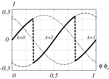
FIG. 1.: Total current for the three-$\mathrm{CuO}_{4}$ ring, as a function of the magnetic flux. Here $U=5\ t$, $|\tau|=0.001\,t$. The current is in units of $e|\tau|/h$. The thick line marks the ground state current.

Next, we report the effects of an inter-unit hopping $\tau_{\rm Cu}$ between Cu sites only; this does not break the $S_{4}^{|\Lambda|}$ symmetry and therefore its consequences on pair propagation and SFQ are drastically different. In order to study the propagation of a bound pair we again assume the total number of particles $2|\Lambda|+2=8$. The full system threaded by the flux has a $C_{3}\otimes S_{4}^{3}$ symmetry because the O sites are not involved in the inter-unit Hamiltonian. We computed the ground state energy versus flux for the case $\Delta_{\mathrm{CuO}_{4}}(4)<0$; $\tau_{\rm Cu}$ produces much smaller effects than $\tau$ for $|\tau_{\rm Cu}|\ll|\Delta_{\mathrm{CuO}_{4}}(4)|$. Therefore we are free to take the inter-unit hopping as large as $|\tau_{\rm Cu}|=\;0.1t$ without causing a drastic change; the dependence of the ground state energy is still weak, see Fig.(2). At $\phi=0$, the correction[19] due to $|\tau_{\rm Cu}|$ to ground state energy is only $\sim 10^{-3}t$. However, the most spectacular change is that the system now behaves like a paramagnet.

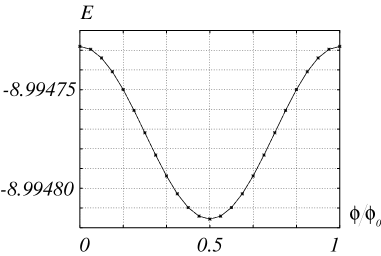
FIG. 2.: Ground state energy $E$ of the three-unit ring in units of $t$, as a function of the concatenated magnetic flux. $E$ is $k$-independent (see text). Here $U=5\ t$, $|\tau_{\rm Cu}|=0.1t$.

The reason of this unusual behavior is the local symmetry, which forbids any flux-induced splitting of the three $k$ levels; the effective mass is infinite and the $W=0$ pair, however bound, is localized. Indeed the $S_{4}$ label of each $\mathrm{CuO}_{4}$ unit is a good quantum number. No SFQ is observed because the screening of the magnetic field by the bound pair is forbidden. The small correction to the ground state energy comes from a second-order process. Suppose we prepare the system e.g. in an unperturbed state ${|4,2,2\rangle}$, that is , with 4 particles in the first $\mathrm{CuO}_{4}$ and 2 in the others; the bound pair is localized on the first cluster. The evolution of the wave packet involves virtual states ${|3,3,2\rangle}$ and ${|3,2,3\rangle}$ which are obtained when a particle jumps to the nearby clusters. This particle must be in totalsymmetric state, because the irreps of each unit must be conserved. However, such a process occurs with a tiny amplitude because the energy misfit is severe. This is particularly clear at weak coupling, when we can speak in terms of orbitals, and the lowest-energy $A_{1}$ particle of the first cluster must hop to antibonding $A_{1}$ orbitals of the nearby clusters; the amplitude of this process is further reduced by the overlap of these orbitals with the localized Cu one. Moreover, such virtual processes are insensitive to the flux. Any $\phi$ dependence arises from third-order corrections in which the $A_{1}$ particle virtually goes around the trip clockwise or anticlockwise. In the ground state, of course, it chooses the wise in such a way to gain energy from the magnetic field. This is why a paramagnetic dependence on the flux is seen in Fig.(2) and the correction goes like $-\phi^{2}$ at small $\phi$. This is interesting because it shows how the local symmetry can hinder the tunneling of bound pairs carrying conserved quantum numbers; SFQ is not a necessary consequence of superconductivity if the pairs are not totalsymmetric.

In conclusion, we have found that Hubbard-like repulsive graphs hosting $W=0$ 2-body states can be used to model bound pairs and their propagation. Thus, SFQ may be found in purely repulsive 1$d$ Hubbard models only if the nodes are represented by a non-trivial basis. For rings of $\mathrm{CuO}_{4}$-units and weak O-O links we find a half-integer AB effect which is unambiguosly interpreted as SFQ. Next, we reported a counterexample, namely, the case of Cu-Cu links, when pairing is not leading to SFQ due to the large effective mass of the particles. By manipulating matrices whose dimension is the square root of the overall size of the Hilbert space we were able to exactly diagonalize the Hamiltonian: $\sqrt{m}\times\sqrt{m}$ matrices solve the $m\times m$ problem by means of a suitable disentanglement of the up and down spin configurations.

REFERENCES

- [1] F. V. Kusmartsev, J. Phys.: Condens. Matter 3, 3199 (1991).
- [2] A. J. Schofield, J. M. Wheatley and T. Xiang, Phys. Rev. B 44, 8349 (1991).
- [3] N. Yu and M. Fowler, Phys. Rev. B 45, 11795 (1992).
- [4] F. Nakano, J. Phys. A 33, 5429 (2000).
- [5] Y. Aharonov and D. Bohm, Phys. Rev. 115, 485 (1959); R.G. Chambers, Phys. Rev. Lett. 5, 3 (1960).
- [6] F. C. Zhang and T. M. Rice, Phys. Rev. B 37, 3759 (1988).
- [7] Michele Cini and Adalberto Balzarotti, Il Nuovo Cimento D 18, 89 (1996)
- [8] Michele Cini and Adalberto. Balzarotti, J. Phys. C 8, L265 (1996).
- [9] Michele Cini and Adalberto Balzarotti, Solid State Comm. 101, 671 (1997); Michele Cini, Adalberto Balzarotti, J. Tinka Gammel and A. R. Bishop, Il Nuovo Cimento D 19, 1329 (1997).
- [10] Michele Cini and Adalberto Balzarotti, Phys. Rev. B 56, 14711 (1997).
- [11] Michele Cini, Gianluca Stefanucci and Adalberto Balzarotti, Eur. Phys. J. B 10, 293 (1999).
- [12] Michele Cini, Gianluca Stefanucci and Adalberto Balzarotti, Solid State Commun. 109, 229 (1999).
- [13] Michele Cini Adalberto Balzarotti and Gianluca Stefanucci, Eur. Phys. J. B 14, 269 (2000).
- [14] Michele Cini, Gianluca Stefanucci, Enrico Perfetto and Agnese Callegari, J. Phys.: Condens Matter 14, L709 (2002).
- [15] E. H. Lieb, Phys. Rev. Lett. 62, 1201 (1989).
- [16] W. Kohn, Phys. Rev. 133, A171 (1964).
- [17] E. Dagotto, Rev. Mod. Phys. 66,763 (1994).
- [18] W. A. Little and R. D. Parks, Phys. Rev. Lett. 9, 9 (1962).
- [19] Using as above one finds , and .