Alpha-Relaxation Processes in Binary Hard-Sphere Mixtures

Abstract

Molecular-dynamics simulations are presented for two correlation functions formed with the partial density fluctuations of binary hard-sphere mixtures in order to explore the effects of mixing on the evolution of glassy dynamics upon compressing the liquid into high-density states. Partial-density-fluctuation correlation functions for the two species are reported. Results for the alpha-relaxation process are quantified by parameters for the strength, the stretching, and the time scale, where the latter varies over almost four orders of magnitude upon compression. The parameters exhibit an appreciable dependence on the wave vector; and this dependence is different for the correlation function referring to the smaller and that for the larger species. These features are shown to be in semi-quantitative agreement with those calculated within the mode-coupling theory for ideal liquid-glass transitions.

I Introduction

If one compresses or cools a liquid, there appear slow dynamical processes which are referred to as structural relaxation. These processes are precursors of the liquid-glass transition. The study of these phenomena has been a very active field of research in recent years. Several new experimental techniques were introduced to measure the evolution of structural relaxation spectra within the GHz band. Molecular-dynamics simulation techniques have been improved considerably so that correlation functions of liquids in equilibrium can be obtained for time intervals covering five to six orders of magnitude. The wealth of information obtained on glassy dynamics is a challenge for the theory of amorphous condensed matter. However, consensus on the understanding of the slow dynamics in glass-forming liquids has not yet been achieved cre (2002); pis (2003).

Simple monoatomic liquids crystallize before structural relaxation dynamics is fully developed. Therefore, studies of the glassy dynamics have to be performed on simple molecular systems or suitable mixtures. Recently, for example, a four-component mixture was studied by neutron-scattering spectroscopy. This system transforms to a metallic glass at low temperatures, but it exhibits the same scenario for the evolution of structural relaxation as known for molecules Meyer (2002). The first molecular-dynamics studies of structural relaxation in an equilibrium liquid were performed for a binary mixture of particles interacting by purely repulsive potentials Bernu et al. (1985, 1987); Roux et al. (1989). A binary Lennard-Jones system has been introduced Kob and Andersen (1994), whose interaction potentials are similar to the ones proposed for the description of the glass-forming Ni-P mixture Stillinger and Weber (1982). This system has been used extensively to analyze all facets of glassy dynamics in the equilibrium liquid and also for the quenched non-equilibrium system Kob (2003); Sciortino and Tartaglia (2001). In the mentioned previous studies, mixing was merely introduced as a means of suppressing crystallization. In the present paper, we analyze the influence of mixing on the structural relaxation.

In order to identify the effect of mixing on the glassy dynamics, we have performed molecular-dynamics simulations for four binary hard-sphere mixtures differing in the size ratio of the constituents and in the composition. By increasing the total packing fraction up to $0.605$, the evolution of structural relaxation was detected for a time interval up to five orders of magnitude. As reported earlier Foffi et al. (2003), two scenarios for mixing effects have been identified. For a mixture with a small size disparity of the constituents, the increase of the mixing percentage of the small particles for a fixed total packing fraction leads to a slowing down of the long-time dynamics. In this case, mixing stabilizes the glass state. However, upon mixing particles with a large size disparity, the increase of the percentage of the small particles at fixed packing fraction speeds up the structural relaxation. In this case, mixing stabilizes the liquid. The present paper reports a detailed analysis of the long-time relaxation processes, traditionally referred to as alpha processes, for the two scenarios mentioned.

Glassy dynamics and a liquid-glass transition can also be observed experimentally in colloidal suspensions. In particular, one can prepare glass-forming colloids where the interaction potential is a very good approximation to a hard-sphere repulsion Pusey (1991). Informative light-scattering studies of structural relaxation for such a hard-sphere suspension have been reported van Megen and Underwood (1993). To suppress crystallization, a narrow distribution of particle sizes was chosen. Strictly, such a system is a multi-component mixture. But ignoring the small polydispersity, it can be viewed as a one-component system. In the same sense, one can consider a colloid studied by Henderson et al. Henderson et al. (1996) as an approximation for a binary hard-sphere mixture with a size ratio $0.8$ between the two groups of particles, and a mixture studied by Williams and van Megen Williams and van Megen (2001) as one with size ratio $0.6$. For the first mixture, a dramatic effect of mixing on the nucleation ratio was observed, but no effect on the glassy dynamics has been reported. For the second mixture, it was shown that the time scale for the alpha relaxation decreased upon mixing. Our simulation results Foffi et al. (2003) suggest that the cited experiments do not deal with colloid-specific features. Rather, they exemplify the two scenarios for mixing effects on structural relaxation. Therefore, the present paper provides a detailed list of quantitative predictions for correlation functions of glassy colloids, which can be measured by photon-correlation spectroscopy.

The mode-coupling theory for ideal liquid-glass transitions provides a physical explanation for the evolution of structural relaxation in simple systems and allows for the first-principle evaluation of the density-correlation functions Götze and Sjögren (1992). The results of this theory for the hard-sphere system have been used for a detailed analysis of the light-scattering data obtained for hard-sphere colloids with a small polydispersity van Megen (1995). The theory has been extended recently to a discussion of binary hard-sphere mixtures. In particular, the above mentioned two mixing scenarios had been obtained Götze and Th. Voigtmann (2003). It was possible to describe a major part of the scattering data for a mixture Williams and van Megen (2001) quantitatively by the theoretical results Th. Voigtmann (2003a). These findings provide a motivation to use our simulation results also for a detailed quantitative test of the mode-coupling theory for the alpha-relaxation process.

The paper is organized as follows. In Sec. II, the simulation details are described, representative results for the two mixtures considered are exhibited, and the mode-coupling-theory formulas for the alpha-relaxation process are listed. Then, in Sec. III, it will be explained how the alpha-relaxation processes are parameterized. The results for the parameters are compared with the corresponding ones obtained from the mode-coupling-theory findings. Section IV presents a comparison of the alpha-relaxation master functions for the density-fluctuation correlation functions of the simulation data with the corresponding theoretical results. In Sec. V, the findings are summarized.

II Basic concepts and results

II.1 Specification of the systems

Let $N$ and $\varrho$ denote the total number of particles and the total number density, respectively, of the binary hard-sphere mixture (HSM) to be studied. Further numbers specifying the system are the particle diameters $d_{\alpha}$, the particle masses $m_{\alpha}$, their thermal velocities $v_{\alpha}$, the partial number densities $\varrho_{\alpha}$ and number concentrations $x_{\alpha}=\varrho_{\alpha}/\varrho=N_{\alpha}/N$, as well as the partial packing fractions $\varphi_{\alpha}=(\pi/6)\varrho_{\alpha}d_{\alpha}^{3}$. Here, $\alpha={\text{A}}$ and B labels the big and small particles, respectively. In the present work, the size ratio $\delta=d_{\text{B}}/d_{\text{A}}$, the total packing fraction $\varphi=\varphi_{\text{A}}+\varphi_{\text{B}}$, and the relative packing fraction of the smaller species, $x=\varphi_{\text{B}}/\varphi$, will be used as convenient control parameters to characterize the thermodynamic state.

Density fluctuations of species $\alpha$ for wave vector $\vec{q}$ are constructed from the positions $\vec{r}_{k}^{(\alpha)}$, $k=1,\ldots,N_{\alpha}$, of particles of type $\alpha$: $\varrho_{\alpha}(\vec{q})=\sum_{k}\exp[i\vec{q}\vec{r}_{k}^{(\alpha)}]/\sqrt{N}$. The partial structure factors $S_{\alpha\beta}(q)=\langle\varrho_{\alpha}(\vec{q})^{*}\varrho_{\beta}(\vec{q})\rangle$ provide the simplest statistical information on the equilibrium distribution of particles, i.e., on the structure. Here, $\langle\cdot\rangle$ denotes canonical averaging. The structure factors depend on the wave vector only via $q=|\vec{q}|$. They can be written as $S_{\alpha\beta}(q)=x_{\alpha}\delta_{\alpha\beta}+\varrho x_{\alpha}h_{\alpha\beta}(q)x_{\beta}$, with $h_{\alpha\beta}(q)$ denoting the Fourier transform of the pair-correlation function. The latter can be expressed in terms of the direct correlation functions $c_{\alpha\beta}(q)$ via the Ornstein-Zernike equation: $h_{\alpha\beta}(q)=c_{\alpha\beta}(q)+\varrho\sum_{\gamma}c_{\alpha\gamma}(q)x_{\gamma}h_{\gamma\beta}(q)$ Hansen and McDonald (1986). The $S_{\alpha\beta}(q)$, $h_{\alpha\beta}(q)$, and $c_{\alpha\beta}(q)$ are elements of real symmetric two-by-two matrices. The discussions will be restricted to such stable and metastable states where $S_{\alpha\beta}(q)$ and $c_{\alpha\beta}(q)$ are smooth functions of $q$ and of the control parameters $\varphi$, $\delta$, and $x$.

The main quantities of interest in this paper are the density correlators $\Phi_{\alpha\beta}(q,t)=\langle\varrho_{\alpha}(\vec{q},t)^{*}\varrho_{\beta}(\vec{q})\rangle$. These correlation functions provide the simplest statistical characterization of the structural dynamics. They are real even functions of time $t$, and they form the elements of a symmetric two-by-two matrix. In principle, the correlators can be measured as intermediate coherent scattering functions by neutron-scattering experiments for conventional liquids, or by photon-correlation spectroscopy for colloidal suspensions. A short-time expansion yields $\Phi_{\alpha\beta}(q,t)=S_{\alpha\beta}(q)-(1/2)(qv_{\alpha}t)^{2}x_{\alpha}\delta_{\alpha\beta}+{\mathcal{O}}(t^{3})$ Hansen and McDonald (1986). Within the regime of normal-liquid states, say, $\varphi<0.4$, the short-time dynamics varies on a $30\%$ level upon changes of the control parameters. There are no structural relaxation phenomena apparent in the transient dynamics.

Two mixtures shall be considered in the following. A system with $\delta=0.60$ and $x=0.20$, referred to as the $\delta=0.60$-system, is representative for a mixture with large size disparity. In this case, $54\%$ of the particles are of species B. A system with $\delta=0.83$ and $x=0.37$, referred to as the $\delta=0.83$-system, contains $50\%$ of small particles. It is representative for a mixture with small size disparity. These mixtures have been used before, together with systems of smaller percentages $x$, in order to demonstrate the evolution of mixing anomalies with variations of $x$ Foffi et al. (2003). Since we are not interested in details of the short-time dynamics, the masses of the particles are chosen equal, i.e. $v_{\text{A}}=v_{\text{B}}$. The units of length and time are chosen such that $d_{\text{A}}=1$ and $v_{\text{A}}=v_{\text{B}}=1$. With these units, the natural time scale for the microscopic motion is $t_{\text{mic}}=d_{\text{A}}/v_{\text{A}}=1$.

II.2 Results from molecular dynamic simulations

We perform standard molecular dynamics simulations for binary mixtures of $N=1237$ and $N=700$ hard-sphere particles with size ratios $\delta=0.60$ and $\delta=0.83$, respectively. The algorithm follows the usual event-driven scheme for the simulation of hard-sphere particles Rapaport (1997), where the trajectory of the system is propagated from one collision to the next one. To generate dense enough initial configurations without particle overlaps, we applied the same procedure as described earlier Zaccarelli et al. (2002): Starting from a random distribution of points, particles were separated growing their diameters in successive steps until the desired size was reached. From the initial configuration, each simulation proceeds by an equilibration run, followed by a production run during which positions and velocities are saved for subsequent analysis. In all cases, the equilibration time was larger than the time it takes for the particles’ average displacement to reach one diameter of the large species, $d_{\text{A}}$. Up to four independent runs per state point have been performed to reduce statistical errors. Density correlation functions $\Phi_{\alpha\beta}(q,t)$ and static structure factors $S_{\alpha\beta}(q)$ have been calculated by averaging over the independent runs and over $300$ different wave vectors $\vec{q}$ of the same modulus $q$. The longest simulation run requested about three weeks, i.e. the largest density studied took about three months of CPU time on a fast AMD Athlon processor to be completed.

We checked that no crystallization occurred during the production runs by monitoring the time evolution of the pressure of the system, and by visual inspection of the configurations. We also evaluated the wave-vector resolved structure factor without angular averaging to make sure that no crystalline peaks have developed. Other mixture compositions than the ones presented below have been tried; for $\delta=0.83$ and $x=0.276$ as well as for $\delta=0.60$ and $x=0.10$, it was also possible to study the glassy dynamics in the liquid phase Foffi et al. (2003), despite a stronger tendency to crystallization. A system with $\delta=0.60$ and $x=0.05$ did not stay in the homogeneous liquid phase long enough for a study of structural relaxation.

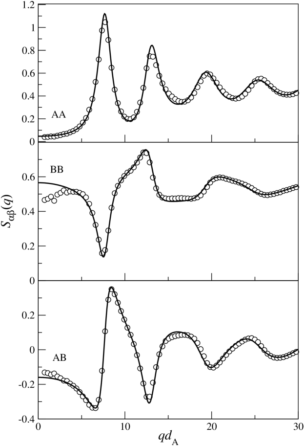
Figure 1: Partial structure factors $S_{\alpha\beta}(q)$, $\alpha,\beta={\text{A}},{\text{B}}$, of a binary hard sphere mixture (HSM) for diameter ratio of the particles $\delta=d_{\text{B}}/d_{\text{A}}=0.60$, a relative packing ratio $x$ of the smaller species of $20\%$, and total packing fraction $\varphi=0.60$. Circles are the molecular-dynamics simulation results, while full lines are the results calculated within Percus-Yevick theory. Here and in the following figures, the diameter of the larger spheres is chosen as the unit of length, $d_{\text{A}}=1$.

Figure 2: The pair distribution functions $g_{\alpha\beta}(r)$ corresponding to the results shown in Fig. 1.

Figures 1 and 2 exhibit a typical set of structure factors and the corresponding pair distribution functions. The results refer to the $\delta=0.60$ system, and the lines are calculated using the Percus-Yevick theory for HSM Lebowitz and Rowlinson (1964); Baxter (1970). Obviously, this approximation theory accounts for the data rather well, even though the packing fraction $\varphi=0.60$ considered is rather large. But there are small systematic deviations of the kind known from the discussion of hard-sphere mixtures at smaller packing fractions Malijevský et al. (1997). For example, the theory overestimates the height of the first and second peak of $S_{{\text{A}}{\text{A}}}(q)$ by about $10\%$. The contact values for the radial distribution function are $11.6$, $6.87$, and $8.76$ for the AA, BB and AB function, respectively, while the Percus-Yevick theory yields $8.88$, $6.32$, and $7.28$, respectively. It will be discussed below that these discrepancies have to be acknowledged if one intends to consider the results of the mode-coupling theory (MCT) quantitatively. Even though the results of Percus-Yevick theory are well-known, a side remark on its qualitative features might be in order. Increasing the size disparity, i.e. decreasing $\delta$ below unity, the height of the first diffraction peak in $S_{{\text{A}}{\text{A}}}(q)$ decreases. Simultaneously, the wing of the peak at $qd_{\text{A}}\approx 9$ increases. Within MCT, the first trend stabilizes the liquid state, while the second trend stabilizes the glass. The first trend dominates at the glass transition for small $\delta$, the second one that for larger $\delta$ Götze and Th. Voigtmann (2003). For the radial distribution functions, these trends correspond to a reduction of the contact values and a decrease of the averaged radius of the first neighbor shell with decreasing $\delta$. Moreover, at larger size disparities, a splitting of the first-neighbor-shell peak into a double peak is observed, as is evident in Fig. 2.

Figure 3: Molecular-dynamics-simulation results for the density correlators $\Phi_{\alpha\beta}(q,t)$, $\alpha,\beta={\text{A}},{\text{B}}$, for the $\delta=0.60$ mixture for wave vector $qd_{\text{A}}=5$. The dotted and dashed lines refer to packing ratios $\varphi=0.40$ and $0.45$, respectively. The full lines are correlators for $\varphi=0.530$, $0.550$, $0.570$, $0.580$, $0.590$, $0.595$, $0.600$, and $0.605$ (from left to right). Here and in the following figures, the unit of time is chosen such that the thermal velocity of the particles is unity.

Figure 4: The analogous results as shown in Fig. 3, but for wave number $qd_{\text{A}}=10$.

Figures 3 and 4 exhibit representative examples for the evolution of the glassy dynamics upon compressing the $\delta=0.60$ mixture. The wave vectors $qd_{\text{A}}=5$ and $qd_{\text{A}}=10$ have been chosen since they exhibit the characteristic differences in mixing effects for small and large wave vectors that have been discussed before Foffi et al. (2003); Götze and Th. Voigtmann (2003). Note that the values of the partial correlation functions can be quite different; in particular the small values of the AB correlator at $qd_{\text{A}}=10$ are responsible for the worse signal to noise ratio observed there.

The correlators for $\varphi=0.40$ are close to exponentials whose characteristic decay time is near the natural time scale $t_{\text{mic}}=1$ for the microscopic dynamics. They are typical for normal-liquid behavior which can be described on a $30\%$ accuracy level by Enskog’s theory for dense gases Boon and Yip (1980). If the packing fraction increases to $\varphi=0.45$, the time scale for the decay of the correlators increases by about $40\%$, so that for $t\approx 5$ all correlators have decayed to below the $5\%$ level of their initial values. Increasing $\varphi$ above $0.45$, a new relaxation pattern evolves for the dynamics outside the transient regime, say for $t>5$. The $\Phi_{\alpha\beta}(q,t)$-versus-$\log t$ diagrams exhibit a two-step relaxation scenario that has repeatedly been observed before in simulation studies and experiments. First, the correlators decrease towards some plateau. The curves become flatter and the plateau lengths increase if $\varphi$ increases. Then, the correlators decrease from the plateau to zero. The dynamics for $t\gtrsim t_{\text{mic}}$ is called structural relaxation. Our simulations document this process, which is characteristic for glass-forming liquids, for a time interval extending over nearly five orders of magnitude.

The second step of the structural relaxation, i.e., the decay below the mentioned plateau is conventionally referred to as the alpha process. The figures demonstrate that the time scale for the alpha process increases the faster with increasing $\varphi$ the larger the packing fraction. The decay cannot be described by an exponential function, rather it is stretched over wider time intervals. Obviously, the whole structural relaxation pattern, in particular the alpha process, shows a subtle dependence on the wave vector $q$. It is the goal of this paper to characterize the alpha process, in particular its $q$ dependence, quantitatively.

II.3 Some mode-coupling-theory equations

Within MCT, the concept of a plateau and of an alpha-relaxation process can be defined precisely in the sense of asymptotic laws describing the dynamics near an idealized liquid-to-glass transition. These laws provide a motivation for the parameterization of the data. In addition, our data shall be used to test quantitatively the results of the theory. In this section, the required formulas are compiled.

Let us introduce an obvious matrix notation to get the following equations in a transparent form. $\boldsymbol{S}(q)$, $\boldsymbol{\Phi}(q,t)$, etc., shall denote two-by-two matrices with elements $S_{\alpha\beta}(q)$, $\Phi_{\alpha\beta}(q,t)$, etc. The Zwanzig-Mori formalism Hansen and McDonald (1986) can be used to derive the exact equation of motion for the density correlators,

$$\boldsymbol{I}(q)\partial_{t}^{2}\boldsymbol{\Phi}(q,t)+\boldsymbol{S}^{-1}(q)\boldsymbol{\Phi}(q,t)+\int_{0}^{t}\boldsymbol{M}(q,t-t^{\prime})\partial_{t^{\prime}}\boldsymbol{\Phi}(q,t^{\prime})\,dt^{\prime}=\boldsymbol{0}\,.$$ (1a)

Here, $$\boldsymbol{I}(q) I_{\alpha\beta}(q)=1/(q^{2}v_{\alpha}^{2}x_{\alpha})\delta_{\alpha\beta} M_{\alpha\beta}(q,t) \boldsymbol{\Phi}(q,t\!=\!0)=\boldsymbol{S}(q) \partial_{t}\boldsymbol{\Phi}(q,t\!=\!0)=\boldsymbol{0} \boldsymbol{M}^{\text{MCT}}(q,t) \boldsymbol{M}^{\text{reg}}(q,t) t_{\text{mic}} \boldsymbol{M}(q,t)=\boldsymbol{M}^{\text{reg}}(q,t)+\boldsymbol{M}^{\text{MCT}}(q,t) \mathcal{F}$$ is a matrix of inertia parameters, . The kernels are fluctuating-force correlation functions, and they reflect the complicated many-body interaction effects. The equation of motion has to be solved with the initial conditions and . The essential step in the theory is the application of Kawasaki’s factorization approximation in oder to identify the kernel contribution , which expresses the coupling of the forces to the density fluctuations. The remainder of the kernel, , is assumed to describe the normal-liquid-state dynamics. It is anticipated to vary regularly in the control parameters and to decay on the scale for the transient motion. One gets , where the mode-coupling kernel is given by the mode-coupling functional ,

$$\boldsymbol{M}^{\text{MCT}}(q,t)={\mathcal{F}}[\boldsymbol{\Phi}(t)](q)\,,$$ (1b)

which reads

$${\mathcal{F}}_{\alpha\beta}[\boldsymbol{\Phi}](q)=\frac{1}{2q^{2}}\frac{\varrho}{x_{\alpha}x_{\beta}}\sum_{\alpha^{\prime}\beta^{\prime}\alpha^{\prime\prime}\beta^{\prime\prime}}\sum_{\vec{k}}V_{\alpha\alpha^{\prime}\alpha^{\prime\prime}}(\vec{q},\vec{k},\vec{p})\Phi_{\alpha^{\prime}\beta^{\prime}}(k)\Phi_{\alpha^{\prime\prime}\beta^{\prime\prime}}(p)V_{\beta\beta^{\prime}\beta^{\prime\prime}}(\vec{q},\vec{k},\vec{p})\,.$$ (1c)

In the sum, the abbreviation $$\vec{p}=\vec{q}-\vec{k} V_{\alpha\alpha^{\prime}\alpha^{\prime\prime}}(\vec{q},\vec{k},\vec{p}) c_{\alpha\beta}(k) \langle\varrho_{\alpha}(\vec{q})^{*}\varrho_{\beta}(\vec{k})\varrho_{\gamma}(\vec{p})\rangle$$ is used. The vertices are expressed in terms of the direct correlation functions and a triple average . Simplifying the latter by the convolution approximation, one gets

$$V_{\alpha\alpha^{\prime}\alpha^{\prime\prime}}(\vec{q},\vec{k},\vec{p})=(\vec{q}\vec{k}/q)c_{\alpha\alpha^{\prime}}(k)\delta_{\alpha\alpha^{\prime\prime}}+(\vec{q}\vec{p}/q)c_{\alpha\alpha^{\prime\prime}}(p)\delta_{\alpha\alpha^{\prime}}\,.$$ (1d)

Note that the mode-coupling functional is determined by the equilibrium structure alone. Specifying the structure factors and a model for $$\boldsymbol{M}^{\text{reg}}(q,t) q^{*} 140 qd_{\text{A}}^{*}=56.8 200 qd_{\text{A}}^{*}=79.8$$, the preceding equations are closed. To proceed towards a numerical solution, one introduces a grid of equally spaced wave numbers extending up to a cutoff . In this paper, we use wave numbers and for the calculations based on the simulated structure factors. Some results based on the Percus-Yevick approximation shall also be shown, and for those we used wave numbers up to . We refer to Ref. Götze and Th. Voigtmann (2003) and the papers quoted there for further details.

The MCT equations exhibit bifurcations for the long-time limits of the solutions. For packing fractions $\varphi$ below some critical value $\varphi^{c}=\varphi^{c}(\delta,x)$, one gets $\boldsymbol{\Phi}(q,t\to\infty)=\boldsymbol{0}$. In this parameter regime, the solutions describe ergodic liquid dynamics. For $\varphi\geq\varphi^{c}$, the long-time limits are non-degenerate symmetric positive definite matrices $\boldsymbol{\Phi}(q,t\to\infty)=\boldsymbol{F}(q)$. For these states, the solutions describe amorphous solids, i.e., ideal glasses. The long-time limits obey the implicit equations

$$\boldsymbol{F}(q)=\boldsymbol{S}(q)-\left[\boldsymbol{S}(q)^{-1}+{\mathcal{F}}[\boldsymbol{F}](q)\right]^{-1}\,.$$ (2)

These equations are defined by the equilibrium structure alone; neither the inertia matrix $\boldsymbol{I}(q)$ nor the regular memory kernel $\boldsymbol{M}^{\text{reg}}(q,t)$ enter. The above equation for $\boldsymbol{F}(q)$ can be solved by a standard iteration procedure Franosch and Th. Voigtmann (2002).

Let $\boldsymbol{F}^{c}(q)$ denote the non-degenerate positive definite matrix of long-time limits at the transition point $\varphi=\varphi^{c}$. For reasons of continuity, $\boldsymbol{\Phi}(q,t)$ has to be close to $\boldsymbol{F}^{c}(q)$ for a large time interval if $|\varphi-\varphi^{c}|$ is small. The correlators are the closer to $\boldsymbol{F}^{c}(q)$ the smaller $|\varphi-\varphi^{c}|$, and the time interval of this close approach extends simultaneously. Thereby, the evolution of the plateaus, which were discussed above in connection with Figs. 3 and 4, is explained by MCT, and the $\boldsymbol{F}^{c}(q)$ are the MCT expressions for the plateaus.

The decay of the correlators from the plateaus to zero for small negative $\varphi-\varphi^{c}$ shall be characterized by some time scale $\tau(\varphi)$. Obviously, $\lim_{\varphi\to\varphi^{c}}\tau(\varphi)=\infty$. Let us consider the dynamics of the relaxation from the plateau on the time scale $\tau$ by writing $t=\tilde{t}\tau$ with $\tilde{t}$ fixed but positive. There holds

$$\lim_{\varphi\to\varphi^{c}}\boldsymbol{\Phi}(q,\tilde{t}\tau)=\boldsymbol{\Psi}(q,\tilde{t})\,,$$ (3)

where $\boldsymbol{\Psi}(q,\tilde{t})$ obeys the equation Fuchs and Latz (1993)

$$\boldsymbol{\Psi}(q,\tilde{t})=\boldsymbol{S}(q)\tilde{\boldsymbol{M}}(q,\tilde{t})\boldsymbol{S}(q)-\boldsymbol{S}(q)\frac{d}{d\tilde{t}}\int_{0}^{\tilde{t}}\tilde{\boldsymbol{M}}(q,\tilde{t}-\tilde{t}^{\prime})\boldsymbol{\Psi}(q,\tilde{t}^{\prime})\,d\tilde{t}^{\prime}\,,$$ (4a)

to be solved with the initial condition $$\boldsymbol{\Psi}(q,\tilde{t}\!=\!0)=\boldsymbol{F}^{c}(q) \tilde{\boldsymbol{M}}(q,\tilde{t})$$. Here, is determined by the mode-coupling functional for the critical point,

$$\tilde{\boldsymbol{M}}(q,\tilde{t})={\mathcal{F}}^{c}[\boldsymbol{\Psi}(\tilde{t})](q)\,.$$ (4b)

The numerical solution of the equation for $$\boldsymbol{\Psi}(q,\tilde{t})$$ is done similar to that for the full equations of motion.

Equation (3) implies the following conclusion. Given some $\tilde{t}_{-}$ and some error margin,

$$\boldsymbol{\Phi}(q,t)=\boldsymbol{\Psi}(q,t/\tau)$$ (5)

is valid within the margin for $\tilde{t}=t/\tau>\tilde{t}_{-}$, provided $\varphi-\varphi^{c}$ is small enough. This is the superposition principle for the MCT alpha process. It describes the correlators in terms of a $\varphi$-independent master function $\boldsymbol{\Psi}(q,\tilde{t})$, and attributes the strong $\varphi$-dependence to that of the scale $\tau$. Presenting the correlators as functions of $\tilde{t}$, the interval for $\tilde{t}$ where they coincide expands to lower values of $\tilde{t}$ if $|\varphi-\varphi^{c}|$ decreases. The master functions $\boldsymbol{\Psi}(q,\tilde{t})$ depend only on the equilibrium structure. Neither the inertia parameters in $\boldsymbol{I}(q)$ nor the regular kernel $\boldsymbol{M}^{\text{reg}}(q,t)$ have any influence on $\boldsymbol{\Psi}(q,\tilde{t})$. These quantities enter the time scale $\tau$ only.

There are complicated but straight-forward formulas to evaluate from ${\mathcal{F}}^{c}$ the so-called von Schweidler exponent $b$, $0<b<1$, a critical amplitude $\boldsymbol{H}^{(1)}(q)$, which is a positive definite matrix, and a correction amplitude $\boldsymbol{H}^{(2)}(q)$ Th. Voigtmann (2003b). These quantities determine the von Schweidler expansion of the master functions,

$$\boldsymbol{\Psi}(q,\tilde{t})=\boldsymbol{F}^{c}(q)-\boldsymbol{H}^{(1)}(q)\tilde{t}^{b}+\boldsymbol{H}^{(2)}(q)\tilde{t}^{2b}\,.$$ (6)

Here, terms of order $\tilde{t}^{3b}$ have been dropped. Thereby an equation is obtained for the beginning of the alpha process.

The MCT equations have been studied before for binary HSM using the Percus-Yevick approximation for the structure factors Götze and Th. Voigtmann (2003). In the present paper, results will be presented using the structure factors $\boldsymbol{S}(q)$ obtained from the simulation work. For the two mixtures we have calculated

$$\varphi^{c}_{\text{MCT}}=0.548,\,b=0.44 \delta=0.60 x=0.20$$ (, ); (7a)

$$\varphi^{c}_{\text{MCT}}=0.545,\,b=0.43 \delta=0.83 x=0.37$$ (, ). (7b)

From the simulation data, the critical packing fractions $\varphi^{c}$ for the liquid-glass transitions of the two mixtures have been determined from the alpha-relaxation times of the density auto-correlation functions, see Sec. III.5, yielding values of $0.606$ and $0.586$, respectively. The errors of $10\%$ and $7\%$, respectively, exhibited by the values noted in Eqs. (7a) and (7b), indicate the uncertainty one should expect for MCT results. It is worth to stress that if one bases MCT on Percus-Yevick approximation for the structure factors, one gets as critical values for the two mixtures $0.520$ and $0.515$, respectively. Hence, the use of correct instead of approximated structure factor input to the theory improves the results for the critical points. It is remarkable that the modest errors of the Percus-Yevick theory, which are exhibited in Fig. 1, lead to noteworthy changes in the MCT results for the critical points.

III Parameterization of the alpha-relaxation processes

III.1 Evolution of the alpha process

Figure 5: Density auto-correlation functions $\Phi_{{\text{A}}{\text{A}}}(q,t)$ and $\Phi_{{\text{B}}{\text{B}}}(q,t)$ of the $\delta{}{=d_{\text{B}}/d_{\text{A}}}=0.60$ system for wave number $qd_{\text{A}}=7.5$, presented as functions of the rescaled time $\tilde{t}=t/\tau$. The upper panel exhibits simulation results for packing fractions $\varphi=0.605$, $0.60$, $0.595$, $0.59$, $0.58$, $0.57$, and $0.53$; the lower panel for $\varphi=0.605$, $0.60$, $0.595$, $0.59$, and $0.58$ (from left to right). For each $\varphi$, the scaling time $\tau$ is chosen such that the curves coincide for large times.

The evolution of the alpha-relaxation scaling law is examined in Fig. 5. The upper panel is a typical example for the majority of correlators obtained in our simulations. For every packing fraction $\varphi$, some time scale $\tau\equiv\tau(\varphi)$ can be defined so that the long-time parts of the correlators coincide if these are considered as functions of $\tilde{t}=t/\tau$. This coinciding part provides the master functions $\Psi_{\alpha\beta}(q,\tilde{t})$ for the alpha process of the fluctuation considered. Upon increasing $\varphi$, the $\tilde{t}$ interval where Eq. (3) holds, expands to lower values of the rescaled time $\tilde{t}$. Thus, the observed scenario confirms the MCT prediction. However, our data also exhibit violations of the above described scenario, which cannot be understood in the framework of MCT. These occur only for the BB correlators of the $\delta=0.60$ mixture for wave vectors around the structure-factor peak position, $qd_{\text{A}}\approx 7$; and this only for the two largest packing fractions examined, $\varphi=0.600$ and $0.605$. The lower panel of Fig. 5 shows a representative example. The following analysis of $\boldsymbol{\Psi}(q,\tilde{t})$ shall therefore be based on those data sets that do not exhibit the described phenomenon; i.e. for $\varphi<0.60$.

Figure 6: Normalized large-particle density auto-correlation functions $\phi_{\text{A}}(q,t)=\Phi_{{\text{A}}{\text{A}}}(q,t)/S_{{\text{A}}{\text{A}}}(q)$ obtained from the simulations for three wave numbers $q$ and packing fraction $\varphi=0.595$ (left full line) for the $\delta=0.60$ mixture. The right full lines are the simulation results for $\varphi=0.590$, rescaled on the first curve for large times $t$. The dashed and dash-dotted lines are fits to the alpha process by the Kohlrausch function, Eq. (8), and the von Schweidler expansion, Eq. (6), with $b=0.44$, respectively. The fit interval for the latter is indicated by the horizontal dotted arrow.

Figure 7: The analogous set of curves as in Fig. 6, but now obtained for the numerical solutions of the MCT equations. The packing fractions for the full curves are $\varphi=0.548$ and $0.545$. The additional dash-dotted lines are the asymptotes given by the first two terms in Eq. (6).

The stretched exponential,

$$\phi_{\alpha}^{\text{K}}(q,\tilde{t})=A_{\alpha}(q)\exp\left[-(\tilde{t}/\tilde{\tau}_{\alpha}(q))^{\beta_{\alpha}(q)}\right]\,,$$ (8)

is an often used empirical function for the description of alpha processes. It was introduced by Kohlrausch for the description of dielectric relaxation data. The description of the alpha-process master function by an amplitude—also called plateau value—$A_{\alpha}(q)$, a time scale $\tilde{\tau}_{\alpha}(q)$, and a Kohlrausch exponent $\beta_{\alpha}(q)$ shall be used here as well. The dashed lines in Fig. 6 exhibit representative examples for an analysis of the normalized auto-correlation functions $\phi_{\text{A}}(q,t)=\Phi_{{\text{A}}{\text{A}}}(q,t)/S_{{\text{A}}{\text{A}}}(q)$. The figures contain rescaled data for $\varphi=0.595$ and $0.590$, in oder to identify a major part for the interval of rescaled times $\tilde{t}$, for which the superposition principle is valid. Similarly, Fig. 7 exhibits examples for a fit of the stretched exponentials to the numerical solutions of the MCT equations. The $q$ vectors are as close to the ones of Fig. 6 as permitted by the use of discrete wave vector grids. Note that the choice of the overall time scale is irrelevant for the discussion of the master functions $\boldsymbol{\Psi}(q,\tilde{t})$.

Figures 6 and 7 confirm an observation often made earlier: the fits by Eq. (8) provide a good description of a major part of the alpha process. However, there are also systematic deviations between the fit function $\phi_{\alpha}^{\text{K}}(q,\tilde{t})$ and the master functions $\Psi_{\alpha\alpha}(q,\tilde{t})$. This holds in a similar manner for the fits to the data and to the MCT results. The fit contains unavoidable systematic errors, because the fit parameters depend somewhat on the time interval chosen for the fit optimization. In our analysis, the fit was done so that the large-$\tilde{t}$ part is described best. Thereby, the errors of the fit appear solely for the small-$\tilde{t}$ part of the master functions.

Equation (6) suggests another fit formula, which is valid for the small-$\tilde{t}$ part of the master functions. But the small-$\tilde{t}$ part can be identified only to the limited extend to which the scaling interval can be established. Consequently, also the fit using the von Schweidler series contains unavoidable uncertainties. The dotted lines in Fig. 6 exhibit representative examples for such fits. Fits could be achieved with von Schweidler exponents $b$ chosen between $0.40$ and $0.50$. Therefore, the predicted exponents, Eq. (7), are confirmed within an uncertainty of $\pm 0.05$. All the results shown are obtained with the cited theoretical exponents. The remaining fit parameters shall be discussed below.

Note that these results can depend somewhat on the time window chosen for the fit, which is $3.5<t<200$ for the fits discussed here. Similarly, the dotted lines in Fig. 7 exhibit the results of Eq. (6) for the MCT results. But here, the functions $\boldsymbol{F}^{c}(q)$, $\boldsymbol{H}^{(1)}(q)$, and $\boldsymbol{H}^{(2)}(q)$, as well as the scale $\tau$ are calculated from the MCT equations. In this sense, the dotted lines are not fit results. The discrepancies between the dotted and the full lines represent the ones between the full solution of the MCT equations of motion and the specified second-order asymptotic description of the solution. It is reassuring that the discrepancies between the full and the dotted lines in Fig. 6 exhibit similar trends as the ones shown in Fig. 7. A quantitative account of the differences between the results shown in the two figures is included in the discussions of the following sections.

III.2 The plateau values

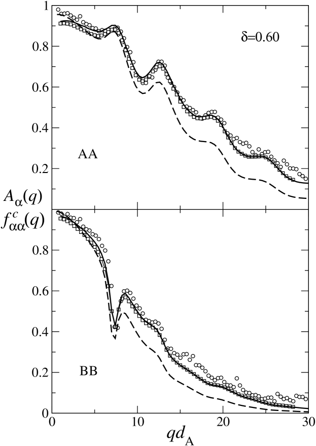
Figure 8: Circles and squares represent the Kohlrausch amplitudes $A(q)$ determined by fitting Eq. (8) to the simulation data and MCT solutions, respectively, for the normalized auto-correlation functions $\Phi_{\alpha\alpha}(q,t)/S_{\alpha\alpha}(q)$ of the big particles, $\alpha={\text{A}}$ (top panel), and the small particles, $\alpha={\text{B}}$ (bottom panel), of the $\delta=0.60$ mixture. The full and dashed lines show the MCT plateau values $f^{c}_{\alpha\alpha}(q)=F^{c}_{\alpha\alpha}(q)/S_{\alpha\alpha}(q)$ calculated with the simulation results for the structure factor and the Percus-Yevick approximation for the $S_{\alpha\beta}(q)$, respectively.

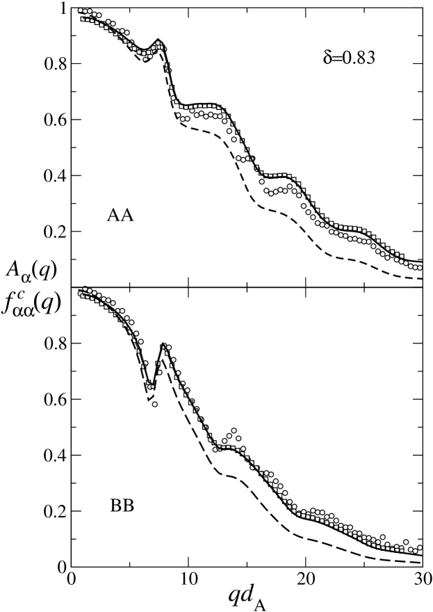
Figure 9: Analogous results as in Fig. 8, but for the mixture with size ratio $\delta=0.83$.

The circles in Figs. 8 and 9 exhibit the plateau values of the two-step relaxation process, $A_{\alpha}(q)$, obtained by fitting Eq. (8) to the simulation data for the normalized auto-correlation functions $\phi_{\alpha}(q,t)$. For $qd_{\text{A}}<6$, the $A_{\alpha}(q)$ are very large; they almost reach their upper limit unity for $q$ tending to zero. This is a typical mixing phenomenon. For one-component systems, $A(q)\approx 0.4$ is expected for small $q$ Bengtzelius et al. (1984); Fuchs and Latz (1993). The width $q_{1/2}$ of the $A_{\alpha}(q)$-versus-$q$ curves, defined by $A_{\alpha}(q_{1/2})=1/2$, is about $7\%$ larger for $\alpha={\text{A}}$ in Fig. 8 than in Fig. 9. This means that the large particles are better localized in the mixture with the larger size disparity. For the smaller B particles, the opposite trend is observed. Similarly, the plateaus for the A correlators exhibit some small peak near the position $qd_{\text{A}}=7.5$ of the structure-factor peak, while the B-correlator plateau values exhibit a pronounced minimum there. For the $\delta=0.60$ mixture, $A_{\text{A}}(q)$ exhibits a minimum near $qd_{\text{A}}=11$, which is accompanied by a maximum near $qd_{\text{A}}=12$. Instead, the $\delta=0.83$ system has a shoulder for $A_{\text{A}}(q)$ for $9<q<12$. All these details are reproduced semi-quantitatively by the results obtained from the MCT values, which are shown as squares in the figures. There are only a few cases where the plateau values deduced from the data differ by up to $10\%$ from the ones deduced from the MCT results: the B plateaus for the $\delta=0.60$ system for $qd_{\text{A}}\approx 16$ or the A plateaus for the $\delta=0.83$ system for $qd_{\text{A}}\approx 17$, for example.

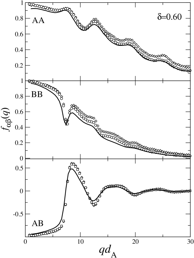
Figure 10: The circles exhibit the plateau values $f_{\alpha\beta}(q)$ for the $\delta=0.60$ mixture, obtained by fitting the simulation data for the normalized correlators $\Phi_{\alpha\beta}(q)/\sqrt{S_{\alpha\alpha}(q)S_{\beta\beta}(q)}$ to the von Schweidler expansion, Eq. (6), see text. $\alpha={\text{A}}$ refers to the big particles, $\alpha={\text{B}}$ to the small ones. The fit was optimized to the data for $\varphi=0.59$. The full lines are the MCT results for the normalized plateaus $f^{c}_{\alpha\beta}(q)=F^{c}_{\alpha\beta}(q)/\sqrt{S_{\alpha\alpha}(q)S_{\beta\beta}(q)}$. For $\alpha=\beta$, they agree with the lines shown in Fig. 8. The squares are fit results optimized for the data for $\varphi=0.595$.

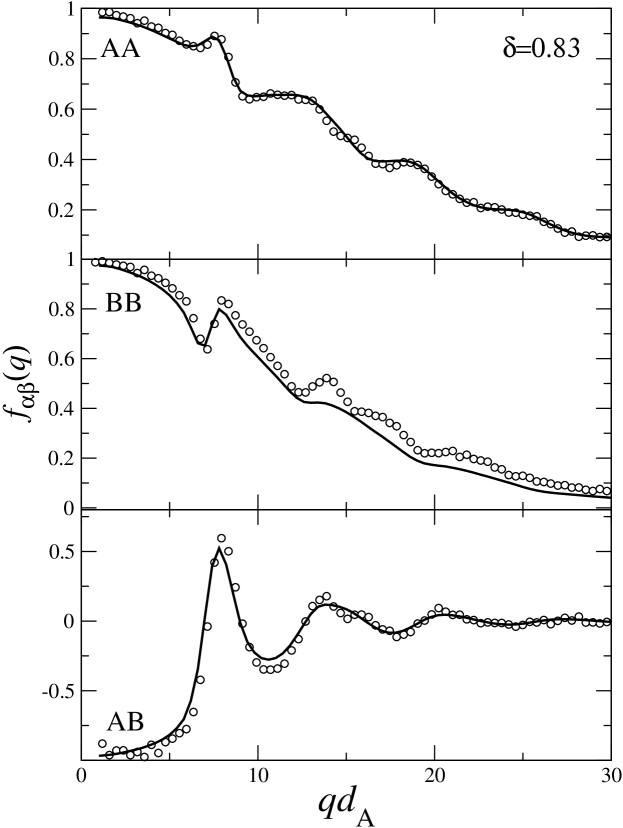
Figure 11: The analog of Fig. 10, but for the $\delta=0.83$ system. The fits are based on the data for $\varphi\approx 0.582$.

The symbols in Figs. 10 and 11 show the results for the plateau values $f_{\alpha\beta}(q)$ obtained from fitting Eq. (6) to the simulation data, normalized by $\Phi_{\alpha\beta}(q,t)/\sqrt{S_{\alpha\alpha}(q)S_{\beta\beta}(q)}$. The fit results obtained for the $\delta=0.60$ mixture for $\varphi=0.590$ and those for $\varphi=0.595$ differ by about $5\%$. This difference thus appears as the inherent uncertainty of the data analysis. No such difference could be identified for the $\delta=0.83$ mixture. The full lines in the figures exhibit the MCT plateau values $f^{c}_{\alpha\beta}(q)=F^{c}_{\alpha\beta}(q)/\sqrt{S_{\alpha\alpha}(q)S_{\beta\beta}(q)}$. For the diagonal functions, $\alpha\beta={\text{A}}{\text{A}}$ and $\alpha\beta={\text{B}}{\text{B}}$, these lines are identical to the full lines shown in Figs. 8 and 9. Those lines should help to compare the plateau results $A_{\alpha}(q)$ with the corresponding fit results for the $f_{\alpha\alpha}(q)$. Obviously, all qualitative features of the plateau fits based on the Kohlrausch function agree with the ones based on the von Schweidler series, both for the fits to the simulation data and for those to the MCT results. The MCT results for $f^{c}_{{\text{A}}{\text{A}}}(q)$ of the $\delta=0.83$ mixture are in perfect agreement with the simulation data, while $f_{{\text{B}}{\text{B}}}(q)$ is underestimated systematically by MCT. But the difference is only about $5\%$, except for $qd_{\text{A}}\approx 14$, where the discrepancy reaches about $10\%$. The deviations for $f_{{\text{A}}{\text{B}}}(q)$ are of similar size. For the system with larger size disparity, the discrepancies between data and MCT result is somewhat larger, but it is not seriously larger than the inherent uncertainty of the fits.

Figure 7 exhibits also the leading term of the von Schweidler expansion. In general, accounting for the next-to-leading term of ${\mathcal{O}}(\tilde{t}^{2b})$ increases the range of validity of the von Schweidler expansion dramatically Fuchs and Latz (1993). Indeed, a data analysis with a $q$-independent exponent $b$ is possible only if the ${\mathcal{O}}(\tilde{t}^{2b})$ term is included Sciortino et al. (1996). However, if $\varphi$ is not close enough to $\varphi^{c}$, it may happen that the ${\mathcal{O}}(\tilde{t}^{3b})$ terms cancel ${\mathcal{O}}(\tilde{t}^{2b})$ contributions. In such case, the fit range may shrink upon inclusion of the ${\mathcal{O}}(\tilde{t}^{2b})$ terms Franosch et al. (1997). This accident is demonstrated by Fig. 7 for $qd_{\text{A}}=10.2$. Such phenomenon cannot be foreseen in an unbiased data analysis, which then, necessarily, must lead to errors in the fit amplitudes. This explains why the sign of the correction amplitude identified in the lower panel of Fig. 6 differs from the one shown in the lower panel of Fig. 7.

An obvious source of errors in the MCT results is due to using incorrect equilibrium-structure information in the mode-coupling functional. It was mentioned in connection with Eq. (7) that replacing the structure factors by their Percus-Yevick approximations increases remarkably the difference between the MCT results for the critical packing fractions and the results derived from the simulation data. The dashed lines in Figs. 8 and 9 exemplify the same phenomenon for the plateau values. These are the MCT results for the $f^{c}_{\alpha\alpha}(q)$ based on the use of the Percus-Yevick structure factors. This approximation for the equilibrium structure leads to underestimations of the plateau values by more than $10\%$. Figures 8 and 9 demonstrate that MCT is so sensitive to the small deviations between $S_{\alpha\beta}(q)$ and the Percus-Yevick results which are exhibited in Fig. 1, that they lead to serious flaws in the quantitative predictions for the dynamics.

Figure 12: MCT plateau values $f^{c}(q)$ for the one-component hard-sphere system, calculated with the simulated structure factor (solid line), with the Percus-Yevick approximation (dashed line), and with the Verlet-Weis expression for $S(q)$ (dash-dotted line). The values for $qd<5$ based on the simulated structure factor are unreliable and have been cut off in the figure.

The difference between the MCT results for the $f^{c}_{\alpha\beta}(q)$ based on the Percus-Yevick approximation and those using $S_{\alpha\beta}(q)$ as obtained from numerical simulations is of similar size for both the $\delta=0.60$ and the $\delta=0.83$ system. It is not a specialty of mixtures, as is demonstrated by Fig. 12. There, the comparison is repeated for the one-component hard-sphere system (HSS). The MCT result for the critical point based on the Percus-Yevick structure factor is $\varphi^{c}_{\text{PY}}=0.516$, and the corresponding plateau values $f^{c}_{\text{PY}}(q)$ are shown as a dashed line. The Verlet-Weis modification of the Percus-Yevick structure factor Verlet and Weis (1972) is an empirical improvement of $S(q)$, in particular for the contact values. Using this as input for the MCT, one gets as the critical point $\varphi^{c}_{\text{VW}}=0.525$. The corresponding $f^{c}_{\text{VW}}(q)$, which are shown as the dash-dotted line, are systematically larger than the ones based on the Percus-Yevick results for $S(q)$. We could obtain simulation data for the structure factor of the metastable HSS for packing fractions up to $\varphi=0.54$. Beyond this packing fraction, crystallization was always taking place before particles could diffuse one nearest neighbor distance, making it impossible to generate data meeting our equilibration criteria. Extrapolating the smoothly $\varphi$-dependent $S(q)$ up to $\varphi=0.55$, we calculated as the critical point $\varphi^{c}_{\text{HSS}}=0.546$ and obtained the full line as the plateau values. It is remarkable that the differences between $f^{c}(q)$ and $f^{c}_{\text{VW}}(q)$ for $qd_{\text{A}}>10$ are larger than those between $f^{c}_{\text{VW}}(q)$ and $f^{c}_{\text{PY}}(q)$. Note that we find, using the simulation results for the structure factors, $\varphi^{c}(\delta\!=\!0.83)<\varphi^{c}_{\text{HSS}}<\varphi^{c}(\delta\!=\!0.60)$, i.e., the system with small size disparity shows a change of $\varphi^{c}$ upon mixing that is qualitatively different from the one seen for large size disparity. This MCT result is qualitatively the same as predicted originally on the basis of the Percus-Yevick approximation Götze and Th. Voigtmann (2003) and is confirmed by our simulations Foffi et al. (2003).

III.3 Von Schweidler-expansion amplitudes

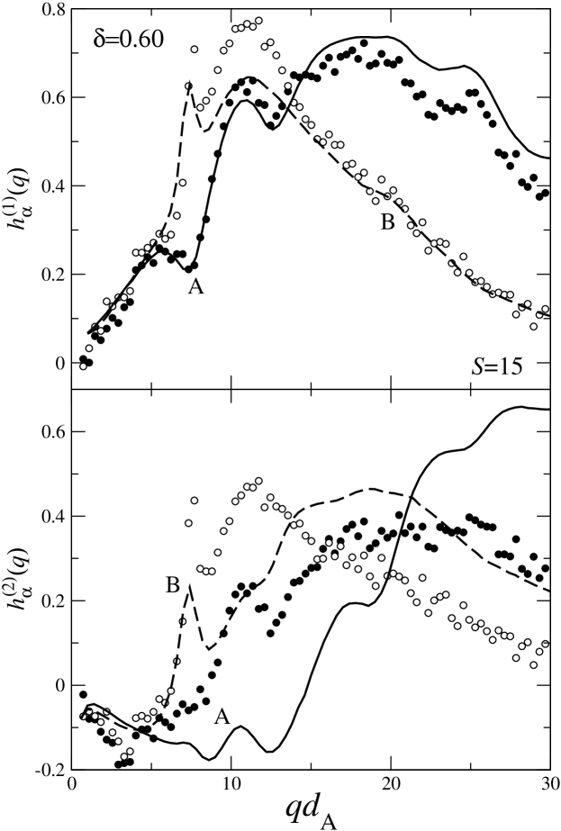
Figure 13: Amplitudes $h_{\alpha}^{(1,2)}(q)=H_{\alpha\alpha}^{(1,2)}(q)/S_{\alpha\alpha}(q)$ for the von Schweidler-law expansion of the normalized density auto-correlation functions $\Psi_{\alpha\alpha}(q,\tilde{t})/S_{\alpha\alpha}(q)$ for the $\delta=0.60$ mixture. The dots and circles are the results of fitting Eq. (6) to the simulation data for $\alpha={\text{A}}$ (large) and $\alpha={\text{B}}$ (small particles), respectively. The full and dashed lines are the corresponding results calculated from the MCT equations. Scale factors $S=15$ and $S^{2}$ are used for the comparisons of the $h_{\alpha}^{(1)}(q)$ and $h_{\alpha}^{(2)}(q)$, respectively, to account for the different time scales $\tau$ used in the analysis of the simulation data and of the calculations.

The amplitudes $H_{\alpha\beta}^{(1)}(q)$ in Eq. (6) are the most important parameters quantifying the dynamics in a time interval where the correlators are close to their plateaus. The upper panel of Fig. 13 exhibits a set of representative results. It compares the amplitudes $h_{\alpha}^{(1)}(q)$ of the normalized master functions $\Psi_{\alpha\alpha}(q,\tilde{t})/S_{\alpha\alpha}(q)$ obtained from the analysis of the simulation data for the $\delta=0.60$ mixture with the corresponding quantities calculated within MCT. For the quantitative comparison, a scale factor $S$ has to be adjusted since the arbitrariness of the time scale $\tau$ implies an arbitrariness in the prefactor $\tau^{-b}$ of $h_{\alpha}^{(1)}(q)=H_{\alpha\alpha}^{(1)}(q)/S_{\alpha\alpha}(q)$. The $h_{\alpha}^{(1)}$-versus-$q$ curves exhibit a subtle structure. While $h_{\text{A}}^{(1)}(q)$ has a maximum for $qd_{\text{A}}\approx 5.7$ followed by a minimum for $qd_{\text{A}}\approx 7.4$, i.e. for a wave vector near the structure-factor peak position, $h_{\text{B}}^{(1)}(q)$ increases monotonically to a maximum for $qd_{\text{A}}\approx 7.4$. While $h_{\text{A}}^{(1)}(q)$ increases for $qd_{\text{A}}>7.4$ monotonically to a maximum for $qd_{\text{A}}\approx 11$, $h_{\text{B}}^{(1)}(q)$ exhibits a sharp minimum for $q$ slightly above $7.4$ before it also reaches a maximum for $qd_{\text{A}}\approx 11$. For $qd_{\text{A}}>11$, $h_{\text{B}}^{(1)}(q)$ decreases monotonically, while $h_{\text{A}}^{(1)}(q)$ has a minimum for $qd_{\text{A}}\approx 12.7$ and then exhibits a broad maximum. These features are reproduced by the MCT results. The MCT results agree with the data on a $10\%$ level, except for the B amplitudes for $qd_{\text{A}}$ near $10$, where there are $20\%$ discrepancies.

The amplitudes $h_{\alpha}^{(2)}(q)$, which describe corrections to von Schweidler’s law $\Psi_{\alpha\alpha}(q,\tilde{t})/S_{\alpha\alpha}(q)=f^{c}_{\alpha\alpha}(q)-h_{\alpha}^{(1)}(q)\tilde{t}^{b}$, exhibit a zero at some wave vector $q_{\alpha}^{*}$. For $q<q_{\alpha}^{*}$, the amplitudes are negative, and for $q>q_{\alpha}^{*}$ they are positive. These features and also the value $q_{\text{B}}^{*}\approx 6$ are reproduced by the MCT results. Notably, the MCT results for $qd_{\text{A}}\leq 12$ still share some qualitative features with the results obtained from the fit to the simulation data, e.g. the sharp peak followed by a sharp minimum in $h_{\text{B}}^{(2)}(q)$ at $qd_{\text{A}}\approx 7$, and the peak in $h_{\text{A}}^{(2)}(q)$ at $qd_{\text{A}}\approx 11$. Otherwise, one notices serious discrepancies between data and MCT results. For example, MCT predicts a particularly large range of validity of von Schweidler’s law for the density fluctuations of the large particles for a wave vector $qd_{\text{A}}\approx 15$. But the data analysis is done best for this case by using a correction amplitude near $0.2$. The identified discrepancies signalize the limitations in the determination of a correction amplitude for an asymptotic law from data which cannot be chosen sufficiently close to the singularity.

III.4 The stretching exponents

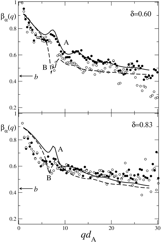
Figure 14: The stretching exponents $\beta_{\alpha}(q)$ obtained by fitting the Kohlrausch function, Eq. (8), to the alpha-relaxation master functions for the density auto-correlation functions of the two mixtures with size ratios $\delta$ of the particles $0.60$ and $0.83$. The arrows in the two panels mark the von Schweidler exponents $b$, Eqs. (7). The dots and circles are obtained by fits to the simulation data for the big particles, $\alpha={\text{A}}$, and the small ones, $\alpha={\text{B}}$, respectively. The full and dashed lines are the corresponding results obtained by fits to the solutions of the MCT equations.

The exponent $\beta$ in Eq. (8) provides a convenient overall measure for the alpha-relaxation stretching. It quantifies in an averaged manner deviations of the alpha-relaxation process from a Debye law, $\phi(t)\propto\exp(-\tilde{t}/\tilde{\tau})$. The latter is the universal result for the dynamics of a variable coupled to a white-noise field. Figure 14 shows that for $2<q<6$, the exponent decreases considerably with increasing $q$. There is no difference between the fluctuations for the large and the small particles in this wave-vector interval; and the stretching is larger for the system with smaller size disparity. For the wave vectors near the structure-factor-peak position, $qd_{\text{A}}\approx 7$, the stretching of the B-fluctuations of the $\delta=0.60$ mixture is much bigger than the one of the A-fluctuations: $\beta_{\text{B}}\approx 0.5$ versus $\beta_{\text{A}}\approx 0.75$. There is an indication of the same phenomenon for the $\delta=0.83$ mixture. For larger wave vectors, $\beta_{\text{A}}$ is somewhat larger than $\beta_{\text{B}}$ for the mixture with large size disparity. For the $\delta=0.83$ mixture, $\beta_{\text{A}}$ equals $\beta_{\text{B}}$ for $qd_{\text{A}}>8$ within the noise of the data.

For $qd_{\text{A}}<6$, the MCT results overestimate $\beta_{\alpha}(q)$ by about $10\%$. The $qd_{\text{A}}\approx 7$ anomaly and also the large-$q$ variation for the $\delta=0.60$ mixture are described well by the theory. For the system with small size disparity, MCT overestimates the $qd_{\text{A}}\approx 7$ anomaly, and there is a slight trend to underestimate $\beta_{\alpha}(q)$ for large $q$.

For large wave vectors, the MCT alpha-process-master functions approach the Kohlrausch law. In this asymptotic regime, $\beta_{\alpha}(q)=b$ Fuchs (1994). Figure 14 illustrates that this theoretical result is consistent with the simulation data.

III.5 The alpha-relaxation time scale

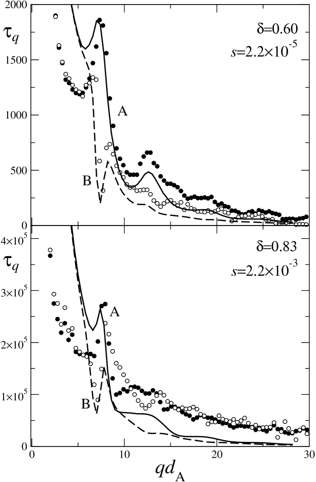
Figure 15: Alpha-relaxation time scales $\tau_{\alpha}(q)$ obtained by fitting Eq. (8) to the data (symbols) and MCT results (lines). The coding is the same as used in Figs. 13 and 14. A multiplication factor $s$ is applied to the MCT results in order to account for the different time scales relative to that used for the data.

The fit of Eq. (8) to the long-time parts of the correlators yields the time scales $\tilde{\tau}_{\alpha}(q)$ for the alpha processes up to an overall scale $\tau$. The results for the fits allow for a comparison of the scales for the fluctuations of the large particles with those for the small ones. They also allow to discuss the $q$ dependence of the relaxation times. In order to compare the scales from the data with those calculated from MCT, one has to fit an overall scale factor $s$.

Figure 15 exhibits the results for the two mixtures. For $qd_{\text{A}}\leq 6$, $\tilde{\tau}_{\text{A}}(q)=\tilde{\tau}_{\text{B}}(q)$, and both scales decrease with increasing wave vector $q$. These features are reproduced by MCT, but the theory overestimates the time scales seriously. For wave vectors near the structure-factor-peak position, $\tilde{\tau}_{\text{A}}$ exhibits a pronounced maximum, and $\tilde{\tau}_{\text{B}}$ has a sharp minimum. The ratios of the scales is about $5$ and $3$ for the systems with large and small size disparity, respectively. This feature is reproduced well by MCT. For the $\delta=0.60$ mixture, $\tilde{\tau}_{\text{A}}(q)$ exhibits a maximum for $qd_{\text{A}}\approx 13$, while $\tilde{\tau}_{\text{B}}(q)$ has a shoulder there. For $qd_{\text{A}}\geq 15$, the relaxation times decrease with increasing $q$. The time scales for the large particles are somewhat larger than those for the small particles. These features are reproduced qualitatively by MCT, but the theory underestimates the time scales by a factor $2$ to $3$ for wave vectors above the structure-factor-peak position. For the $\delta=0.83$ mixture, the scale $\tilde{\tau}_{\text{A}}(q)$ exhibits a shoulder for $10<q<13$ in accord with MCT. The time $\tilde{\tau}_{\text{B}}(q)$ exhibits a minimum for $qd_{\text{A}}\approx 12$, while MCT shows a kink there. Again, MCT underestimates the $\tilde{\tau}_{\alpha}(q)$ for $qd_{\text{A}}\geq 10$.

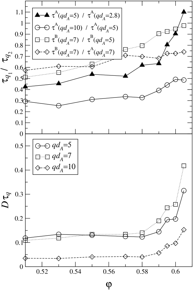
Figure 16: Ratio of alpha-relaxation times $\tau^{\alpha}(q)$ (upper panel) and product of alpha-relaxation times with the large-particle diffusivity $D=D_{\text{A}}$ (lower panel) for the $\delta=0.60$ system as functions of the packing fraction $\varphi$ (see text). The lines are guides to the eye.

Let us consider the variation of the alpha-relaxation time scales as functions of the packing fraction $\varphi$. To this end, we have determined a time scale $\tau^{\alpha}(q,\varphi)$ for this process by arbitrarily choosing $\phi_{\alpha\alpha}(q,t\!=\!\tau^{\alpha}(q,\varphi))=0.1$, for those values of $q$ where the plateau values are still appreciably larger than $0.1$. Equation (3) formulates the scale coupling of the MCT results. While the time scales of two alpha processes, say $\tau_{1}$ and $\tau_{2}$, diverge for vanishing distance parameter $\varepsilon=(\varphi^{c}-\varphi)/\varphi^{c}$, the ratio $\tau_{1}/\tau_{2}$ is a smooth function of $\varepsilon$. For example, let $\tau_{1}$ and $\tau_{2}$ refer to the alpha processes of the correlator $\phi_{{\text{A}}{\text{A}}}(q,t)$ of the $\delta=0.60$ system for $qd_{\text{A}}=10$ and $qd_{\text{A}}=5$, respectively. If $\varepsilon$ increases up to about $0.05$, $\tau_{1}/\tau_{2}$ decreases linearly with $\varepsilon$ by about $4\%$. The simulation results behave similarly, as is shown in the upper panel of Fig. 16. If the packing fraction increases from $0.50$ to $0.605$, the alpha-relaxation time scales of the density-fluctuation correlators increase by more than three orders of magnitude. Still, the shown three representative ratios for the scales vary by less than a factor two. Hence, the scale-coupling prediction is verified on a $10\%$ level for the three ratios shown in the upper panel of Fig. 16 by the open symbols. These examples are representative for density-fluctuation scales with intermediate and large wave numbers. If one of the wave numbers decreases to small values, the violation of the scale coupling becomes larger, as is demonstrated by the full symbols in Fig. 16. The diffusivity $D$ is proportional to the inverse of the alpha-relaxation scale $\tau_{D}$ of the mean-squared displacement. Hence, a $\tau\cdot D$-versus-$\varphi$ diagram demonstrates the coupling of the scales for the processes described by $\tau$ and that for the diffusivity. The lower panel of Fig. 16 shows the results for the $\delta=0.60$ system. Here, $\tau$ refers to the scale for the density fluctuations of the A particles, and the $D$ are the simulation data for the A-particle diffusivities Foffi et al. (2003). The scale coupling holds for $\varepsilon\geq 0.05$. However, approaching the transition point more closely, contrary to the MCT results, the scale for the diffusivity decouples from that for the density fluctuations. The diffusivity does not decrease with decreasing $\varepsilon$ as strongly as $1/\tau$. The results of our simulations for the $\delta=0.83$ system behave similarly. The described decoupling is in qualitative agreement with the behavior found earlier for the simulation results of a binary Lennard-Jones system Kob and Andersen (1994) and for a model for water Starr et al. (1999).

Figure 17: $\tau^{-1/\gamma}$ with $\gamma=3$ as function of the packing fraction $\varphi$. The $\tau$ are the alpha-relaxation times for the large-particle density-fluctuation correlators $\phi_{{\text{A}}{\text{A}}}(q,t)$ calculated from the MCT equations, defined by $\phi_{{\text{A}}{\text{A}}}(q,\tau)=0.1$. The wave numbers $q$ are $10.2$ (diamonds), $7.4$ (squares), and $5.0$ (circles). The dotted lines are the asymptotic laws $\tau^{-1/\gamma}\propto(\varphi^{c}-\varphi)$ with $\varphi^{c}(\delta=0.60)=0.548$ and $\varphi^{c}(\delta=0.83)=0.545$.

Figure 18: $\tau^{-1/\gamma}$ with $\gamma=3$ (left scale) as function of $\varphi$. The $\tau$ are the alpha-relaxation times for the large-particle correlation functions at wave number $qd_{\text{A}}=10$ (diamonds), $7$ (squares), and $5$ (circles), defined by $\phi_{{\text{A}}{\text{A}}}(q,\tau)=0.1$. The upper and lower triangles are $D^{1/\gamma}$ (right scale) for the diffusivities of the small and big particles, respectively. The dashed lines are linear interpolations of the data for large $\varphi$.

MCT predicts a power-law divergence in the asymptotic limit of vanishing $\varepsilon$ for the common scale $\tau$ in Eq. (3): $\tau\propto\varepsilon^{-\gamma}$. The exponent $\gamma$ is determined by the von Schweidler exponent $b$ Götze and Sjögren (1992). The value $b\approx 0.44$ used throughout the preceding discussions implies $\gamma\approx 3.0$. Figure 17 demonstrates this property for the MCT results for $\tau_{\text{A}}(q)$ for three representative wave numbers $q$ in form of a rectification diagram. In agreement with typical results for the simple HSS Franosch et al. (1997), the asymptotic description holds well for $\varepsilon$ up to about $0.05$, and there appear deviations if $\varphi$ differs from $\varphi^{c}$ by more than $5\%$. Analogous rectification diagrams for the simulation data are shown in Fig. 18. Linear extrapolations of the data to large $\varphi$ for three wave numbers $q$ yield estimates for the critical packing fractions: $\varphi^{c}(\delta=0.60)=0.606\pm 0.001$ and $\varphi^{c}(\delta=0.83)=0.585\pm 0.001$. The rectification curves for the diffusivity relaxation times for both types of particles are included in the figure as $D^{1/\gamma}$-versus-$\varphi$ plots. The data seem to follow the power-law predictions, but lead to slightly different estimates of $\varphi^{c}$, also depending on the species $\alpha={\text{A}},{\text{B}}$. For the $\delta=0.60$ system, we get $\varphi^{c}_{D_{\text{A}}}\approx 0.609$ and $\varphi^{c}_{D_{\text{B}}}\approx 0.619$, while for the $\delta=0.83$ system, $\varphi^{c}_{D_{\text{A}}}\approx 0.588$ and $\varphi^{c}_{D_{\text{B}}}\approx 0.590$. The decoupling of the diffusivity scales from the ones for the density fluctuations mentioned above yields this overestimation of the critical packing fractions. Let us emphasize that the described estimations of $\varphi^{c}$ have been done with the bias of a given exponent $\gamma=3.0$. An unbiased three-parameter fit of the scale as a function of $\varphi$ by the formula $\tau=C(\varphi^{c}-\varphi)^{-\gamma}$ suffers from correlations between the fit parameters $\varphi^{c}$ and $\gamma$. Indeed, such fits to the diffusivities of the two species lead to differing exponents $\gamma$ Foffi et al. (2003), in disagreement with MCT. A similar result has also been found in a simulation of a binary Lennard-Jones mixture Kob and Andersen (1994). Fig. 18 however shows that on the basis of our simulation data, one can, given the restricted range of validity of the asymptotic law, not distinguish between these different $\gamma$ values. Note that the largest discrepancy, either in $\gamma$ or in $\varphi^{c}$, emerges for the B particles in the $\delta=0.60$ system. Unbiased fits lead to larger uncertainties for $\varphi^{c}$, since a decrease of the fit parameter $\varphi^{c}$ can partly be compensated by a decrease of the fit parameter $\gamma$. One could get the crossing points of the $D^{1/\gamma^{\prime}}$-versus-$\varphi$ curves closer to that of the $\tau^{-1/\gamma}$-versus-$\varphi$ curves in Fig. 18, if one would use some $\gamma^{\prime}<\gamma$. Such formulation of the decoupling phenomenon is suggested by Fig. 16, since the increase in $D\cdot\tau$ for $\varphi$ increasing above $0.58$ can be fitted by $(\varphi^{c}-\varphi)^{x}$, $x=\gamma^{\prime}-\gamma<0$.

A comparison of Figs. 17 and 18 leads to two questions, which we cannot answer. Why is the range of the distances $\varepsilon$, where the power-law asymptote describes the alpha scales, so much larger for the simulation results than for the MCT solutions? Why do the deviations of $\tau^{-1/\gamma}$ for larger $\varepsilon$ from the small-$\varepsilon$ asymptote have a different sign for the simulation results than for the MCT solutions?

IV The alpha-process shape functions

Figure 19: Alpha-master functions $\tilde{\phi}_{\alpha\beta}(q,t)=\phi_{\alpha\beta}(q,t)/f_{\alpha\beta}(q)$ for the $\delta=0.60$ mixture ($\alpha={\text{A}}$ refers to large particles, $\alpha={\text{B}}$ to small ones). The circles and triangles represent the simulation data for $\varphi=0.595$ and $0.59$, respectively, scaled as in Fig. 5. The solid lines are MCT results for the master function $\Psi_{\alpha\beta}(q,t)/F^{c}_{\alpha\beta}(q)$, and a solution for a distance $\varepsilon=(\varphi-\varphi^{c})/\varphi^{c}\approx-0.015$ from the critical point. Time has been rescaled for all curves in order to match the alpha-time scale of the simulation data at $qd_{\text{A}}=5$, $\alpha\beta={\text{A}}{\text{A}}$. The results refer to wave vectors $qd_{\text{A}}=5$, $7.5$, $10$, and $12.5$ (from top to bottom), where the curves for different $q$ have been shifted vertically by $0.3$ for enhanced clarity.

Figure 20: As in Fig. 19, but for $\delta=0.83$ and $\varphi\approx 0.582$ (circles) and $\varphi\approx 0.575$ (triangles). The solid lines are the theoretical master curve and a curve with $\varepsilon\approx-0.01$.

The preceding parameterization of the correlation functions shows that there is no universal master function for the alpha-relaxation processes. For example, the stretching of the density-fluctuation auto-correlation functions for the large particles generally differs from the one for the small particles, and it depends on the wave vector of the fluctuations. It is a challenge for a microscopic theory to describe the alpha-process shape functions for different probing variables. Figures 19 and 20 present our simulation results for the two mixtures under consideration for four representative wave vectors in comparison with the MCT curves. All results are rescaled by the plateau values and by the time scales discussed in Sec. III. The data are shown for two packing fractions in order to document the asymptotic regime of validity of the superposition principle. The MCT master function is complemented by a curve for some small $\varphi^{c}-\varphi$, in order to indicate the effect of preasymptotic corrections to the alpha-process asymptote.

Figure 19 shows that, typically, the decay of the correlators of the $\delta=0.60$ system from $90\%$ to $5\%$ of their respective plateau values is stretched on a time interval of about three decades. With two exceptions, this decay is described well by the MCT master functions for the alpha process. The first exception is the AA correlator for $qd_{\text{A}}=7.5$ for rescaled times $t\approx 4\times 10^{3}$. Here, the data decay less rapidly as the exponential long-time tail obtained by MCT. The second exception concerns the BB correlator for $qd_{\text{A}}=10$ and $qd_{\text{A}}=12.5$. Here, the data fall on the master functions only for such long times, where the correlator is below $70\%$ of the plateau value. But, the MCT results for $(\varphi-\varphi^{c})/\varphi^{c}\approx-0.015$, which are added in rescaled presentation as full lines in Fig. 19, exhibit the same phenomenon. The reason for this is the large size of the critical amplitude $h_{\text{B}}^{(1)}(q)$ for these wave vectors, cf. Fig. 13. They cause particularly large preasymptotic corrections to the alpha-scaling law near the plateau. Thus, the specified exceptions are not a defect of MCT, but a confirmation of a subtlety of that theory.

The test of the alpha-process shape functions for $\delta=0.83$, Fig. 20, exhibits a series of problems. Deviations of the data from exponential decay for the very long rescaled times $t\approx 5\times 10^{5}$ occur for $qd_{\text{A}}=5$ and $qd_{\text{A}}=7.5$ for all three correlators. The AB correlator for $qd_{\text{A}}=12.5$ shows more stretching than the MCT solutions. Furthermore, the BB correlators for $qd_{\text{A}}=10$ and $qd_{\text{A}}=12.5$ miss the plateau. However, the latter is an obvious mistake of the data analysis, which could be eliminated by correcting the plateau value. We did not carry out this correction in order to emphasize that $5\%$ errors in the determination of the plateau values are almost unavoidable in an unbiased data analysis. The reduction of the scaling regime for the BB correlator for $qd_{\text{A}}=10$ and $12.5$ occurs for the $\delta=0.83$ system as discussed above for the $\delta=0.60$ system; and it can be explained in the same manner.

The most severe problem exhibited by Fig. 20 is the following. Even for $\varepsilon\approx 0.02$, in the simulation, several correlators stay within a $5\%$ interval around the plateau for time intervals as large as $2.5$ decades or more. This holds, e.g., for the AA correlator for $qd_{\text{A}}=7.5$, for the BB correlator for $qd_{\text{A}}=5$, and for the AB correlator for $qd_{\text{A}}=7.5$ and $10$. The full lines show that this feature cannot be explained by MCT. Even if the distance parameter $\varepsilon=(\varphi^{c}-\varphi)/\varphi^{c}$ is as small as $10^{-2}$, the calculated correlators cross their plateaus much steeper than exhibited by the simulation data.

V Conclusions

Molecular-dynamics simulations have been presented for two dense binary mixtures of hard spheres. One mixture deals with a size ratio $\delta=0.60$ for the two particle species and the other with $\delta=0.83$. The first system is representative for the situation where mixing stabilizes the liquid state, and the other for the one where mixing stabilizes the glass Foffi et al. (2003). The data demonstrate the evolution of a two-step relaxation scenario with increasing packing fraction $\varphi$, Figs. 3 and 4, which is similar to the one detected previously for other systems. In this paper, a comprehensive analysis of the second relaxation step, usually referred to as the alpha process, is presented. It deals with the decay of the correlators from some plateau to zero. The process was identified as that part of the correlators exhibiting the superposition principle predicted originally by mode-coupling theory (MCT), Fig. 5. This pattern is exhibited by all our simulation data except for the correlators for the small particles of the $\delta=0.60$ system for wave numbers near the structure-factor peak position, and this for the two largest densities $\varphi=0.600$ and $0.605$, Fig. 5. This violation of the superposition principle might indicate that MCT ignores relaxation processes which become important close to the liquid-glass transition point in this mixture. A possibility that we cannot exclude, however, are precursors of crystallization or phase separation.

The simulation data for the alpha process have been fitted by Kohlrausch functions and by the von Schweidler expansion, Eqs. (8) and (6), respectively. These fits provide two estimates of the plateau values. Usually, these estimates agree on a $5\%$ accuracy level, Fig. 6. Analyzing the MCT results with Kohlrausch functions, one gets plateaus which agree with the correct values within $5\%$, Fig. 7. This means, that both mentioned fit procedures yield reliable estimations for the plateaus, within the indicated uncertainty level. These plateau values exhibit a remarkable structure as functions of the wave number $q$. There are qualitative differences in the structure of the plateau functions referring to the A particles and the B particles. And there are quantitative differences between the results for the two mixtures. All these results are described quantitatively by the MCT results except for some rare cases, where data and theory differ by up to $10\%$, Figs. 8–11.

MCT requires the structure factors as input for the equations of motion. The MCT results reported in this paper are based on the simulation results for the studied systems, Fig. 1. Replacing these structure factors by their Percus-Yevick approximation results, MCT still reproduces all qualitative features of the mentioned plateau functions. However, one systematically underestimates the data. The error of the MCT results caused by the specified erroneous structure information can be as large as $20\%$, Figs. 8 and 9. These findings do not deal with mixture-specific effects. They apply also for the simple hard-sphere system, Fig. 12.

The stretching of the alpha processes is parameterized by the Kohlrausch exponents $\beta_{\alpha}(q)$, and the relative time scales are quantified by the scales $\tau_{\alpha}(q)$. These quantities vary with the wave vector and they depend on the index $\alpha$ for the species, $\alpha={\text{A}},{\text{B}}$. MCT reproduces the $\beta_{\alpha}(q)$ reasonably, but there occur discrepancies up to $20\%$. The trends for the $\tau_{\alpha}(q)$ are reproduced by the theory, but there occur large quantitative errors, Figs. 14 and 15.

Writing the von Schweidler expansion, Eq. (6), for the diagonal correlators in the form $\Psi_{\alpha\alpha}(q,\tilde{t})=F_{\alpha\alpha}^{c}(q)\left[1-[h_{\alpha}^{(1)}(q)/F_{\alpha\alpha}^{c}(q)]{\tilde{t}}^{b}+[h_{\alpha}^{(2)}(q)/F_{\alpha\alpha}^{c}(q)]{\tilde{t}}^{2b}\right]$, one notices that $h_{\alpha}^{(1)}(q)$ defines a relative time scale $\tilde{\tau}_{\alpha}(q)=[h_{\alpha}^{(1)}(q)/F_{\alpha\alpha}^{c}(q)]^{-1/b}$ while $h_{\alpha}^{(2)}(q)$ specifies the shape. The amplitudes $h_{\alpha}^{(1)}(q)$ are reproduced reasonably by MCT, but there occur errors up to $20\%$. MCT describes the trend of the $q$- and species-dependence of the correction amplitudes $h_{\alpha}^{(2)}(q)$, but there are large discrepancies between data and theory, Fig. 13.

The contradicting conclusions concerning the description of the alpha process parameters arrived at in the preceding two paragraphs indicate that the described problems are ones of the fitting procedures. Indeed, Figs. 19 and 20 show that MCT describes the alpha-process master functions well.

Qualitative discrepancies between MCT and simulation data concern the ratio of the time scales $\tau(q)$ for the alpha-relaxation processes for the density fluctuations of intermediate wave numbers $q$ and the time scale $\tau_{D}$ determining the strong variation of the particle diffusivity $D$, $D\propto 1/\tau_{D}$. If the packing fraction of the $\delta=0.60$ system increases from $0.51$ to $0.605$, $\log\tau(q)$ increases by $3.5$, but $\log\tau_{D}$ increases only by $3.0$. The ratio $\tau(q)/\tau_{D}\propto\tau(q)D$ is practically constant if $\varphi$ increases from $0.51$ to $0.58$, i.e. there is perfect scale coupling within this density interval. But increasing $\varphi$ further, the ratio increases by up to a factor $4$, Fig. 16. MCT overestimates the trend to particle localization near the glass transition point. This overestimation of $\tau_{D}$ seems to be the reason why the calculated relaxation times $\tau(q)$ exceed the data for small $q$, as is demonstrated in Fig. 15 for $qd_{\text{A}}\leq 5$. The longest time scale for $q\to 0$ is that for the collective diffusion process: $\tau^{\text{coll}}(q)\propto 1/(q^{2}D^{\text{coll}}(q))$. The coupling of this mode to the density fluctuations causes the divergence of $\tau(q)$ for $q\to 0$. One should expect that an underestimation of the tagged-particle diffusivity $D$ implies the same mistake for the collective diffusivity $D^{\text{coll}}$. This explains, why the decoupling of $\tau(q)$ and $\tau(q^{\prime})$ increases if $q^{\prime}$ decreases to small values, as shown by the filled symbols in Fig. 16.

The increase of the time scales $\tau(q)$ with increasing packing fraction is described well by the asymptotic power law for the MCT results, Fig. 18. However, the mentioned scale decoupling implies that the extrapolation to zero of the $(1/\tau_{D})^{1/\gamma}$-versus-$\varphi$ graphs leads to an estimation of the critical packing fraction $\varphi^{c}$, which exceeds the value obtained from the $(1/\tau(q))^{1/\gamma}$-versus-$\varphi$ extrapolation by $0.6\%$ Foffi et al. (2003).

Finally, a feature of our simulation data should be emphasized which concerns the time regime where the correlators cross their plateaus. It deals with times larger than the ones describing the short-time transient but preceding the regime of validity of the alpha-relaxation scaling law. Within MCT, this regime is described for large densities by the $\beta$-relaxation scaling laws. In this respect, the MCT results for the hard-sphere mixtures behave as the ones for the simple hard-sphere system Götze and Th. Voigtmann (2003). Figure 20 shows, however, that the correlators for the $\delta=0.83$ system are close to the plateaus for time intervals exceeding the ones for corresponding MCT results by more than an order of magnitude. Hence, the $\beta$-relaxation theory cannot account for the simulation data dealing with the plateau crossing. In that respect our simulation data for the hard-sphere mixture are also qualitatively different from the ones measured for quasi-bidisperse hard-sphere colloids Williams and van Megen (2001) and from the simulation data for the binary Lennard-Jones mixture Kob (2003).