Freezing transitions in fluids of long elongated molecules

Abstract

We have used the density-functional theory to locate the freezing transitions and calculate the values of freezing parameters for a system of long elongated molecules which interact via the Gay-Berne pair potential. The pair correlation functions of isotropic phase which enter in the theory as input informations are found from the Percus-Yevick integral equation theory. At low temperatures the fluid freezes directly into the smectic $A$ phase on increasing the density. The nematic phase is found to stabilize in between the isotropic and smectic $A$ phases only at high temperatures and high densities. These features of the phase diagram are in good agreement with the computer simulation results.

I Introduction

A system consisting of anisotropic molecules is known to exhibit liquid crystalline phases in between the isotropic liquid and the crystalline solid. The liquid crystalline phases that commonly occur in a system of long elongated molecules are nematic and smectic (Sm $A$) phases 1 . In the nematic phase the full translational symmetry of the isotropic fluid phase (denoted as $R^{3}$) is maintained but the rotational symmetry $O(3)$ or $SO(3)$ (depending upon the presence or absence of the center of symmetry) is broken. In the simplest form of the axially symmetric molecules the group $SO(3)$ [or $O(3)$] is replaced by one of the uniaxial symmetry $D_{\infty h}$ or $D_{\infty}$. The phase possessing the $R^{3}\wedge D_{\infty h}$ (denoting the semi-direct product of the translational group $R^{3}$ and the rotational group $D_{\infty h}$) symmetry is known as uniaxial nematic phase.

The smectic liquid crystals, in general, have a stratified structure with the long axis of molecules parallel to each other in layers. This situation corresponds to partial breakdown of translational invariance in addition to the breaking of the rotational invariance. Since a variety of molecular arrangements are possible within each layer, a number of smectic phases are possible. The simplest among them is the Sm $A$ phase. In this phase the center of mass of molecules in a layer are distributed as in a two dimensional fluid but the molecular axes are on the average along a direction normal to the smectic layer (i.e. the director ${\bf\hat{n}}$ is normal to the smectic layer). The symmetry of the Sm $A$ phase is $(R^{2}\times Z)\wedge D_{\infty h}$ where $R^{2}$ corresponds to a two dimensional liquid structure and Z for a one-dimensional periodic structure. The other non-chiral and non-tilted smectic phase seen in a system of long elongated molecules is smectic $B_{h}$(Sm $B_{h}$) phase. In each smectic layer of the Sm $B_{h}$ phase, the director is parallel to the layer normal as in the Sm $A$ phase, and there is short-range positional but long range bond-orientational hexagonal orders in smectic plane. The azimuthally symmetrical x-ray ring of Sm $A$ is replaced by a six-fold modulated diffused pattern 2 . The phase is thus characterized by a $D_{6h}$ point group symmetry and is uniaxial like Sm $A$.

All these phases including that of the isotropic liquid and the crystalline solids are characterized by the average position and orientation of molecules and by the intermolecular spatial and orientational correlations. The factor responsible for the existence of these distinguishing features is the anisotropy in both the shape of molecules and the attractive forces between them. The relationship between the intermolecular interactions and the relative stability of these phases is very intriguing and not yet fully understood. For a real system one faces the problem of knowing accurate intermolecular interaction as a function of intermolecular separation and orientations. This is because the mesogenic molecules are so complex that none of the methods used to calculate interactions between molecules can be applied without drastic approximations. Consequently, one is forced to use the phenomenological descriptions, either as a straightforward model unrelated to any particular physical system , or as a basis for describing by means of adjustable parameters between two molecules. Since our primary interest here is to relate the phases formed and their properties to the essential molecular factor responsible for the existence of liquid crystals and not to calculate the properties of any real system, the use of the phenomenological potential is justified. One such phenomenological model which has attracted lot of attention in computer simulations is one proposed by Gay and Berne 3 .

In the Gay-Berne (GB) pair potential model, the molecules are viewed as rigid units with axial symmetry. Each individual molecule $i$ is represented by a center-of-mass position ${\bf r_{i}}$ and an orientation unit vector ${\bf\hat{e}_{i}}$ which is in the direction of the main symmetry axis of the molecule. The GB interaction energy between a pair of molecules (i, j) is given by

$$u({\bf r_{ij}},{\hat{\bf e_{i}}},{\hat{\bf e_{j}}})=4\epsilon({\hat{\bf e_{i}}},{\hat{\bf e_{j}}})(R^{-12}-R^{-6})$$ (1)

where

$$R=\frac{r_{ij}-\sigma({\hat{\bf e_{i}}},{\hat{\bf e_{j}}},{\hat{\bf r}_{ij}})+\sigma_{0}}{\sigma_{0}}$$ (2)

Here $\sigma_{0}$ is a constant defining the molecular diameter, $r_{ij}$ is the distance between the center of mass of molecules $i$ and $j$ and $\hat{\bf r}_{ij}={{\bf r}_{ij}}/{|{\bf r}_{ij}|}$ is a unit vector along the center-center vector ${\bf r}_{ij}={\bf r}_{i}-{\bf r}_{j}$. $\sigma({\hat{\bf e_{i}}},{\hat{\bf e_{j}}},{\hat{\bf r}_{ij}})$ is the distance (for given molecular orientation) at which the intermolecular potential vanishes and is given by

$$\sigma({\hat{\bf e_{i}}},{\hat{\bf e_{j}}},\hat{\bf r}_{ij}) = \sigma_{0}\left[1-\chi\left(\frac{({\hat{\bf e_{i}}}.{\hat{\bf r}_{ij}})^{2}+({\hat{\bf e_{j}}}.{\hat{\bf r}_{ij}})^{2}-2\chi({\hat{\bf e_{i}}}.{\hat{\bf r}_{ij}})({\hat{\bf e_{j}}}.{\hat{\bf r}_{ij}})({\hat{\bf e_{i}}}.{\hat{\bf e_{j}}})}{1-\chi^{2}({\hat{\bf e_{i}}}.{\hat{\bf e_{j}}})^{2}}\right)\right]^{-\frac{1}{2}}$$ (3)

The parameter $\chi$ is a function of the ratio $x_{0}(\equiv\sigma_{e}/\sigma_{s})$ which is defined in terms of the contact distances when the particles are end-to-end $(e)$ and side-by-side $(s)$,

$$\chi=\frac{x_{0}^{2}-1}{x_{0}^{2}+1}$$ (4)

The orientational dependence of the potential well depth is given by a product of two functions

$$\epsilon({\hat{\bf e_{i}}},{\hat{\bf e_{j}}},\hat{\bf r}_{ij})=\epsilon_{0}\epsilon^{\nu}({\hat{\bf e_{i}}},{\hat{\bf e_{j}}})\epsilon^{\prime\mu}({\hat{\bf e_{i}}},{\hat{\bf e_{j}}},\hat{\bf r}_{ij})$$ (5)

where the scaling parameter $\epsilon_{0}$ is the well depth for the cross configuration $(\hat{\bf e_{i}}.{\hat{\bf e_{j}}}=\hat{\bf r}_{ij}.\hat{\bf e_{i}}=\hat{\bf r}_{ij}.\hat{\bf e_{j}}=0)$. The first of these functions

$$\epsilon({\hat{\bf e_{i}}},{\hat{\bf e_{j}}})=[1-\chi^{2}({\hat{\bf e_{i}}}.{\hat{\bf e_{j}}})^{2}]^{-\frac{1}{2}}$$ (6)

favors the parallel alignment of the particle and so aids liquid crystal formations. The second function has a form analogous to $\sigma({\hat{\bf e_{i}}},{\hat{\bf e_{j}}},{\hat{\bf r}_{ij}})$, i.e.

$$\epsilon^{\prime}({\hat{\bf e_{i}}},{\hat{\bf e_{j}}},{\hat{\bf r}_{ij}})=\left[1-\chi^{\prime}\left(\frac{({\hat{\bf e_{i}}}.{\hat{\bf r}_{ij}})^{2}+({\hat{\bf e_{j}}}.{\hat{\bf r}_{ij}})^{2}-2\chi^{\prime}({\hat{\bf e_{i}}}.{\hat{\bf r}_{ij}})({\hat{\bf e_{j}}}.{\hat{\bf r}_{ij}})({\hat{\bf e_{i}}}.{\hat{\bf e_{j}}})}{1-\chi^{\prime 2}({\hat{\bf e_{i}}}.{\hat{\bf e_{j}}})^{2}}\right)\right]$$ (7)

The parameter $\chi^{\prime}$ is determined by the ratio of the well depth as

$$\chi^{\prime}=\frac{k^{\prime 1/\mu}-1}{k^{\prime 1/\mu}+1}.$$ (8)

Here $k^{\prime}$ is well-depth ratio for the side-by-side and end-to-end configuration.

The GB model contains four parameters $(x_{0},k^{\prime},\mu,\nu)$ that determine the anisotropy in the repulsive and attractive forces in addition to two parameters $(\sigma_{0},\epsilon_{0})$ that scale the distance and energy, respectively. Though $x_{0}$ measures the anisotropy of the repulsive core, it also determines the difference in the depth of the attractive well between the side-by-side and the cross configurations. Both $x_{0}$ and $k^{\prime}$ play important role in stabilizing the liquid crystalline phases. The exact role of other two parameters $\mu$ and $\nu$ are not very obvious; though they appear to affect the anisotropic attractive forces in a subtle way.

The phase diagram found for the system interacting via GB potential of Eqs. (1.1)-(1.8) exhibits isotropic, nematic and Sm $B$ phases 4 ; 5 for $x_{0}=3.0,k^{\prime}=5.0,\mu=2$, and $\nu=1$. An island of Sm $A$ is, however, found to appear in the phase diagram at value of $x_{0}$ slightly greater than 3.0 5 . The range of Sm $A$ extends to both higher and lower temperatures as $x_{0}$ is increased. Also as $x_{0}$ is increased, the isotropic-nematic ($I-N$) transition is seen to move to lower density (and pressure) at a given temperature. Bates and Luckhurst 6 have investigated the phases and phase transition for the GB potential with $x_{0}=4.4,k^{\prime}=20.0,\mu=1$ and $\nu=1$ using the isothermal-isobaric Monte-Carlo simulations. At low pressure they found isotropic, Sm $A$ and Sm $B$ phases but not the nematic phase. However as the pressure is increased, the nematic phase also get stabilized and a sequence of $I-N$-Sm $A$ and Sm $B$ was found.

In this paper we use the density functional approach to examine the different phases using Gay-Berne potential with the parameters chosen in the ref. 6 and compare our results with the results found by the simulations. The paper is organized as follows. In Sec. II, we describe Percus-Yevick integral equation theory for the calculation of the pair correlation functions of the isotropic phase. We compare our results with those found by simulations. In Sec. III the density-functional formalism has been used to locate the freezing transitions and freezing parameters. The paper ends with a discussion given in Sec. IV.

II Isotropic liquid: Pair Correlation Functions

In the theory of freezing to be discussed in the next section the structural informations of isotropic phase will be used as input data. The structural information of an isotropic liquid is contained in the two particle density distribution $\rho({\bf 1},{\bf 2})$ as the single particle density distribution is constant independent of position and orientation. The two-particle density distribution $\rho({\bf 1},{\bf 2})$ measures the probability of finding simultaneously a molecule in a volume element d${\bf r}_{1}$d${\bf\Omega}_{1}$ centered at$({\bf r}_{1},{\bf\Omega}_{1})$ and a second molecule in a volume element d${\bf r}_{2}$d${\bf\Omega}_{2}$ at $({\bf r}_{2},{\bf\Omega}_{2})$. The pair correlation function $g({\bf 1},{\bf 2})$ is related to $\rho({\bf 1},{\bf 2})$ as

$$g({\bf 1},{\bf 2})=\frac{\rho({\bf 1},{\bf 2})}{{\rho({\bf 1})}{\rho({\bf 2})}}$$ (9)

where $\rho(\bf i)$ is the single particle density distribution. Since for the isotropic fluid $\rho({\bf 1})=\rho({\bf 2})=\rho_{f}=\langle N\rangle/V$, where $\langle N\rangle$ is the average number of molecules in the volume V,

$$\rho_{f}^{2}g({\bf r},{\bf\Omega}_{1},{\bf\Omega}_{2})=\rho({\bf r},{\bf\Omega}_{1},{\bf\Omega}_{2})$$ (10)

where ${\bf r}={\bf r}_{2}-{\bf r}_{1}$. In the isotropic phase $\rho({{\bf 1},{\bf 2}})$ depends only on distance $|{\bf r}_{2}-{\bf r}_{1}|=r$, the orientation of molecules with respect to each other and on the direction of vector ${\bf r}$.

The pair distribution function $g({\bf 1},{\bf 2})$ of the isotropic fluid is of particular interest as it is the lowest order microscopic quantity that contains information about the translational and orientational structures of the system and also has direct contact with intermolecular (as well as with intramolecular) interactions. For an ordered phase, on the other hand, as shown in the next section most of the structural informations are contained in the single particle distribution $\rho({{\bf 1}})$. In the density functional theory of freezing the single particle distribution $\rho({\bf 1})$ of an ordered phase is expressed in terms of the pair correlation function of the isotropic fluid (see Sec III).

The value of $g({\bf 1},{\bf 2})$ as a function of intermolecular separation and orientation at a given temperature and density is found either by computer simulation or by solving the Ornstein-Zernike(OZ) equation

$$h({\bf 1},{\bf 2})=c({\bf 1},{\bf 2})+\rho_{f}\int c({\bf 1},{\bf 3})h({\bf 2},{\bf 3})d{\bf 3}$$ (11)

where $d{\bf 3}=d{\bf r}_{3}d{\bf\Omega}_{3}$ and $h({\bf 1},{\bf 2})=g({\bf 1},{\bf 2})-1$ and $c({\bf 1},{\bf 2})$ are, respectively, the total and direct pair correlation functions(DCF), using a suitable closure relation such as Percus-Yevick(PY) integral equation , hypernetted chain (HNC) relations. Approximations are introduced through these closure relations 7 .

The Percus-Yevick closure relation is written in various equivalent form.The form adopted here is

$$\ c^{PY}({\bf 1},{\bf 2})=f({\bf 1},{\bf 2})[g({\bf 1},{\bf 2})-c({\bf 1},{\bf 2})]$$ (12)

where $f({\bf 1},{\bf 2})=\exp[-\beta u({\bf 1},{\bf 2})]-1$ is Mayer function , $\beta=(k_{B}T)^{-1}$ and $u({\bf 1},{\bf 2})$ is a pair potential of interaction. Since for the isotropic liquid DCF is an invariant pair wise function, it has an expansion in body fixed (BF) frame in terms of basic set of rotational invariants, as

$$\ c(r_{12},{\bf\Omega}_{1},{\bf\Omega}_{2})=\sum_{l_{1}l_{2}m}c_{l_{1}l_{2}m}(r_{12})Y_{l_{1}m}({\bf\Omega}_{1})Y_{l_{2}{\underline{m}}}({\bf\Omega}_{2})$$ (13)

where ${\underline{m}}$=-m. The coefficients $c_{l_{1}l_{2}m}(r_{12})$ are defined as

$$\ c_{l_{1}l_{2}m}(r_{12})=\int c(r_{12},{\bf\Omega}_{1},{\bf\Omega}_{2})Y^{*}_{l_{1}m}({\bf\Omega}_{1})Y_{l_{2}{\underline{m}}}^{*}({\bf\Omega}_{2})d{\bf\Omega}_{1}d{\bf\Omega}_{2}$$ (14)

Expanding all the angle dependent functions in BF frame, the OZ equation reduces to a set of algebraic equation in Fourier space

$$\ h_{l_{1}l_{2}m}(k)=c_{l_{1}l_{2}m}(k)+(-1)^{m}\frac{\rho_{f}}{4\pi}\sum_{l_{3}}c_{l_{1}l_{3}m}(k)h_{l_{3}l_{2}m}(k)$$ (15)

where the summation is over allowed values of $l_{3}$. The PY closure relation is expanded in spherical harmonics in the body (or space) fixed frame. The pair correlation functions are then found by solving these self consistently 8 .

In our earlier work 9 ; 10 we considered $30$ harmonics in expansion of each orientation dependent function (see Eq.(2.5)); i.e. the series were truncated at the value of $l$ indices equal to $6$. Since the accuracy of the results depends on this number and as the anisotropy of the shape taken here is larger than the earlier work, we considered $54$ harmonics. The series of each orientation dependent function was truncated at the value of $l$ indices equal to 8. The numerical procedure for solving Eq(2.7) is the same as discussed in ref.10 .

In Fig.1 we compare the values of g(r*)=1+$h_{000}(r*)/4\pi$ in BF-frame having 30 and 54 harmonic coefficients at $T^{*}(=k_{B}T/\epsilon_{0})=1.40$ and density $\eta(={\pi}\rho_{f}\sigma_{0}^{3}x_{0}/6)$= 0.44 for $x_{0}=4.4$, where $r^{*}=r/\sigma_{0}$ is the reduced interparticle separation. One other projection of the pair-correlation is shown in Fig.2 for the same set of parameters. It is obvious from these figures that even for $x_{0}=4.4$ one gets good results with 30 harmonics.

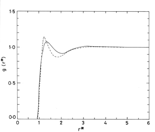
Figure 3: Pair-Correlation function of the centre of mass g($r^{*}$) for GB fluid with parameters $x_{0}=4.4,k^{\prime}=20.0,\mu=1$ and $\nu$ = 1 at $\eta=0.36$ and $T^{*}=1.80$. The solid curve is our PY result and dashed curve is the simulation result of Bates and Luckhurst [6].

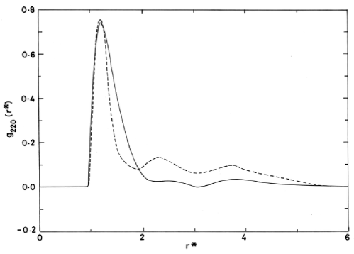
Figure 4: Spherical harmonic coefficient $g_{220}(r^{*})$ in the body-fixed frame. The curves are same as in Fig.3.

In Figs.3 and 4 we compare the values of $g(r^{*})$ and $g_{220}(r^{*})$, respectively, with those obtained by computer simulations 6 for $\eta=0.36$ and $T^{*}=1.80$. From these figures we find that while the PY theory gives qualitatively correct results for the pair correlation functions, quantitatively it underestimates the orientational correlations. The PY peak in $g(r^{*})$ (see Fig.3) is broad and of less hight than the one found from the simulation. Though peak hight in $g_{220}(r^{*})$ compare well, the oscillation at large $r^{*}$ is damped more in PY results than in the simulation data. However, as emphasized in our earlier work the PY theory is reasonably accurate for the GB potential at low temperatures 10 .

III Freezing transitions

In the density functional approach one uses the grand thermodynamic potential defined as

$$-W=\beta A-\beta{\mu_{c}}\int d{\bf x}\rho({\bf x})$$ (16)

where A is the Helmholtz free energy, $\mu_{c}$ the chemical potential and $\rho({\bf x})$ is a singlet distribution function, to locate the transition. It is convenient to subtract the isotropic fluid thermodynamic potential from $W$ and write it as 11

$$\Delta W=W-W_{f}=\Delta W_{1}+\Delta W_{2}$$ (17)

with

$$\frac{\Delta W_{1}}{N} = \frac{1}{\rho_{f}V}\int{d\bf r}{d\bf\Omega}\left\{{\rho({\bf r},{\bf\Omega})\ln\left[\frac{\rho({\bf r},{\bf\Omega})}{\rho_{f}}\right]-\Delta\rho({\bf r},{\bf\Omega})}\right\}$$ (18)

$${\rm and}$$

$$\frac{\Delta W_{2}}{N} = -\frac{1}{2\rho_{f}}\int{d\bf r_{12}}{d\bf\Omega_{1}}{d\bf\Omega_{2}}\Delta\rho({\bf r_{1}},{\bf\Omega_{1}})c({\bf r_{12}},{\bf\Omega_{1}},{\bf\Omega_{2}})\Delta\rho({\bf r_{2}},{\bf\Omega_{2}})$$ (19)

Here $\Delta\rho({\bf x})=\rho({\bf x})-\rho_{f}$, where $\rho_{f}$ is the density of the coexisting liquid.

The minimization of $\Delta W$ with respect to arbitrary variation in the ordered phase density subject to a constraint that corresponds to some specific feature of the ordered phase leads to

$$\ln\frac{\rho({\bf r_{1}},{\bf\Omega_{1}})}{\rho_{f}} = \lambda_{L}+\int d{\bf r_{2}}d{\bf\Omega_{2}}c({\bf r_{12}},{\bf\Omega_{1}},{\bf\Omega_{2}};\rho_{f})\times$$ (20)

$$\Delta\rho({\bf r_{2}},{\bf\Omega_{2}})$$

where $\lambda_{L}$ is Lagrange multiplier which appears in the equation because of constraint imposed on the minimization.

Eq.(3.5) is solved by expanding the singlet distribution $\rho({\bf x})$ in terms of the order parameters that characterize the ordered structures. One can use the Fourier series and Wigner rotation matrices to expand $\rho({\bf r},{\bf\Omega})$. Thus

$$\ \rho({\bf r},{\bf\Omega})=\rho_{0}\sum_{q}\sum_{lmn}Q_{lmn}(G_{q})\exp(i{\bf G}_{q}.{\bf r})D^{l}_{mn}({\bf\Omega})$$ (21)

where the expansion coefficients

$$\ Q_{lmn}(G_{q}) = \frac{2l+1}{N}\int d{\bf r}\int d{\bf\Omega}\rho({\bf r},{\bf\Omega})\times$$ (22)

$$\exp(-i{\bf G_{q}}.{\bf r})D^{*l}_{mn}({\bf\Omega})$$

are the order parameters, ${\bf G_{q}}$ the reciprocal lattice vectors, $\rho_{0}$ the mean number density of the ordered phase and $D^{*l}_{mn}({\bf\Omega})$ the generalized spherical harmonics or Wigner rotation matrices. Note that for a uniaxial system consisting of cylindrically symmetric molecules $m=n=0$ and, therefore, one has

$$\ \rho({\bf r},{\bf\Omega})=\rho_{0}\sum_{l}\sum_{q}Q_{lq}\exp(i{\bf G}_{q}.{\bf r})P_{l}(\cos\theta)$$ (23)

and

$$\ Q_{lq}=\frac{2l+1}{N}\int d{\bf r}\int d{\bf\Omega}\rho({\bf r},{\bf\Omega})\exp(-i{\bf G_{q}}.{\bf r})P_{l}(\cos\theta)$$ (24)

where $P_{l}(\cos\theta)$ is the Legendre polynomial of degree $l$ and $\theta$ is the angle between the cylindrical axis of a molecule and the director.

In the present calculation we consider two orientational order parameters

$$\bar{P}_{l} = \frac{Q_{l0}}{2l+1}=\langle P_{l}(cos\theta)\rangle$$ (25)

with $l$=2 and 4, one order parameter corresponding to positional order along Z axis,

$${\bar{\mu}} = Q_{00}(G_{z})=\langle cos(\frac{2\pi}{d}z)\rangle$$ (26)

($d$, being the layer spacing) and one mixed order parameter that measures the coupling between the positional and orientational ordering and is defined as,

$$\tau = \frac{1}{5}Q_{20}(G_{z})=\langle cos(\frac{2\pi}{d}z)P_{l}(cos\theta)\rangle$$ (27)

The angular bracket in above equations indicate the ensemble average.

The following order parameter equations are obtained by using Eqs.(3.5) and (3.9):

$$\bar{P}_{l} = \frac{1}{2d}\int_{0}^{d}dz_{1}\int_{0}^{\pi}sin\theta_{1}d\theta_{1}P_{l}(cos\theta_{1})\exp[sum]$$ (28)

$${\bar{\mu}} = \frac{1}{2d}\int_{0}^{d}dz_{1}\int_{0}^{\pi}sin\theta_{1}d\theta_{1}cos(\frac{2\pi z_{1}}{d})\exp[sum]$$ (29)

$$\tau = \frac{1}{2d}\int_{0}^{d}dz_{1}\int_{0}^{\pi}sin\theta_{1}d\theta_{1}P_{2}(cos\theta_{1})cos(\frac{2\pi z_{1}}{d})\exp[sum]$$ (30)

and change in density at the transition is found from the relation

$$1+\Delta\rho^{*}=\frac{1}{2d}\int_{0}^{d}dz_{1}\int_{0}^{\pi}sin\theta_{1}d\theta_{1}\exp[sum].$$ (31)

Here

$$sum = \Delta\rho^{*}\hat{C}_{00}^{0}+2{\bar{\mu}}cos(\frac{2\pi z}{d})\hat{C}_{00}^{1}(\theta_{1})+\bar{P}_{2}\hat{C}_{20}^{0}(\theta_{1})+\bar{P}_{4}\hat{C}_{40}^{0}(\theta_{1})+$$ (32)

$$2\tau cos(\frac{2\pi z}{d})\hat{C}_{20}^{1}(\theta_{1})$$

and

$$\hat{C}_{L0}^{q}(\theta_{1}) = ({\frac{2l+1}{4\pi}})^{1/2}\rho_{f}\sum_{l_{1}l}i^{l}(2l_{1}+1)^{1/2}(2l+1)^{1/2}C_{g}(l_{1}Ll;000)P_{l_{1}}(cos\theta_{1})\times$$ (33)

$$\int_{0}^{\infty}c_{l_{1}Ll}(r_{12})j_{l}(G_{q}r_{12})r_{12}^{2}dr_{12}$$

where $C_{g}(l_{1}Ll;000)$ are Clebsch-Gordon coefficients and $G_{q}=2\pi/d$.

In the isotropic phase all the four order parameters become zero. In the nematic phase the orientational order parameters $\bar{P}_{2}$ and $\bar{P}_{4}$ become nonzero but the other two parameters $\bar{\mu}$ and $\tau$ remain zero. This is because the nematic phase has no long range positional order. In the Sm $A$ phase all the four order parameters are nonzero showing that the system has both the long range orientational and positional order along one direction. Equations (3.10)-(3.16) are solved self consistently using the values of direct pair correlation function harmonics $c_{l_{1}l_{2}l}(r)$ evaluated in the previous section at a given value of T* and $\eta$. This calculation is repeated with different values of $d$, the interlayer spacing. By substituting these solutions in Eqs.(3.2)-(3.4) we find the grand thermodynamic potential difference between ordered and isotropic phases; i.e.

$$-\frac{\Delta W}{N} = -\Delta\rho^{*}+\frac{1}{2}\Delta\rho^{*}(2+\Delta\rho^{*})\hat{C}_{00}^{0}+\frac{1}{2}(\bar{P}_{2}^{2}\hat{C}_{22}^{0}+\bar{P}_{4}^{2}\hat{C}_{44}^{0})+{\bar{\mu}}^{2}\hat{C}_{00}^{1}+$$ (34)

$$2{\bar{\mu}}\tau\hat{C}_{20}^{1}+\tau^{2}\hat{C}_{22}^{1}$$

where

$$\hat{C}_{LL^{\prime}}^{q} = (2L+1)^{1/2}(2L^{\prime}+1)^{1/2}\rho_{f}\sum_{l}i^{l}({\frac{2l+1}{4\pi}})^{1/2}C_{g}(LL^{\prime}l;000)\times$$ (35)

$$\int_{0}^{\infty}c_{LL^{\prime}l}(r_{12})j_{l}({G_{q}r_{12}})r_{12}^{2}dr_{12}$$

At a given temperature and density a phase with lowest grand potential is taken as the stable phase. Phase coexistence occurs at the values of $\rho_{f}$ that makes ${-\Delta W}/{N}=0$ for the ordered and the liquid phases. The transition from nematic to the Sm $A$ is determined by comparing the values of $-{\Delta W}/{N}$ of these two phases at a given temperature and at different densities. We have done this analysis at four different temperatures, i.e. at $T^{*}$=1.2, 1.4, 1.6 and 1.8. Our results are summarized in Table 1. We see that at low temperatures, i.e. at $T^{*}$=1.2 and 1.4 the isotropic liquid freezes directly into Sm $A$ on increasing the density. Nematic phase is not stable at these temperatures. However, at $T^{*}$=1.6 the isotropic liquid on increasing the density is found first to freeze into the nematic phase at $\eta=0.49$ and on further increasing the density the nematic phase transforms into Sm $A$ phase at $\eta=0.519$. At high temperature, $T^{*}$=1.8 the transition is found to take place between isotropic and nematic only for the density range considered by us.

Table 1: Values of the order parameters at the transitions for the GB potential with $x_{0}=4.4,k^{\prime}=20,\mu=\nu=1$. Quantities in reduced units are $d^{*}=d/\sigma_{0}$, Pressure $P^{*}=P\sigma_{0}^{3}/\epsilon_{0},\mu^{*}_{c}=\mu_{c}/\epsilon_{0},\;\;{\rm and}\;\;\eta=\pi\rho_{f}\sigma_{0}^{3}x_{0}/6$

$T^{*}$	Transition	$\eta$	$d^{*}$	$\Delta\rho^{*}$	$\bar{\mu}$	${\bar{P}_{2}}$	${\bar{P}_{4}}$	$\tau$	$P^{*}$	$\mu^{*}_{c}$
1.20	I-Sm A	0.390	3.67	0.212	0.64	0.99	0.71	0.52	1.06	6.51
1.40	I-Sm A	0.440	3.90	0.164	0.65	0.95	0.66	0.54	1.72	10.54
1.60	I-N	0.490	0.0	0.087	0.0	0.76	0.49	0.0	2.61	15.49
	N-Sm A	0.519	4.00	0.127	0.49	0.94	0.67	0.42	3.01	17.34
1.80	I-N	0.530	0.0	0.072	0.0	0.75	0.47	0.0	3.57	20.53

Using the results summarized in Table 1 we draw the phase digram in Fig.5 in the density-temperature plane. The full circles represent the points given in Table 1 and lines are drawn to demarcate the phase boundaries.

IV Discussions

The phase diagram shown in Fig.5 is in good qualitative agreement with the one found by computer simulations 6 . At low temperature the nematic is unstable; on increasing the density the fluid freezes directly into Sm $A$ phase. The nematic phase is found to stabilize in-between the isotropic and Sm $A$ phases when $T^{*}\geq$1.5. When we compare the phase diagram given in Fig.5 with the one reported by Bates and Luckhurst 6 we find that while $N$-Sm $A$ boundary is in good agreement, the $I-N$ boundary is shifted towards lower temperatures compared to that given in ref.6 . As a consequence the region of existence of the nematic phase in the phase diagram found by us is relatively narrow. For example, at $P^{*}$=3.0 we find $T_{N-SmA}/T_{I-N}=0.945$ whereas the value found by Bates and Luckhurst 6 is 0.795. We also find that the values of the orientational order parameters and the change in density at the transitions are higher than those given in ref 6 .

The reason for finding the $I-N$ phase boundary at lower temperatures compared to that found in simulation can be traced to the inadequacy of the PY integral equation theory discussed in Sec.II to estimate the values of orientational correlations at higher temperatures. Moreover, as we have shown in our earlier work 10 that the second-order density functional method (discussed in Sec.III) has the tendency to overestimate the orientational order parameters and the change in density. The modified weighted density approximation (MWDA) 10 ; 12 version of density-functional method is expected to improve the agreement. We have checked it by using this theory to locate the $I-N$ transition at T*=1.6 and 1.8. We find that $I-N$ transition at $T^{*}$=1.6 takes place at $\eta=0.471$ with $\Delta\rho^{*}=0.042,\bar{P}_{2}=0.59,\bar{P}_{4}=0.35$ and $P^{*}$=2.38. These values are in better agreement with computer simulation than those given in Table 1. Similarly at $T^{*}$=1.8 the $I-N$ transition takes place at $\eta=0.498$ with $\Delta\rho^{*}=0.038,\bar{P}_{2}=0.61,\bar{P}_{4}=0.35$ and $P^{*}$=3.10 giving better agreement compared to the values found from the second-order density-functional theory. The dashed line in Fig.5 demarcating the $I-N$ boundary represent the results found from the MWDA version of the density functional method. If we take the dashed line as the phase boundary between isotropic and nematic phases then at $P^{*}$=3.0, $T_{N-SmA}/T_{I-N}=0.890$, instead of 0.945.

In the conclusions we wish to emphasize that the freezing transitions in complex fluids can be predicted reasonably well with the density-functional method if the values of pair correlation functions in the isotropic phase are accurately known.

V acknowledgements

The work was supported by the Department of Science and Technology (India) through a project grant.

Figure 1: Pair-Correlation functions of the centre of mass g($r^{*}$) for GB fluid with parameters $x_{0}=4.4,k^{\prime}=20.0,\mu=1$ and $\nu$ = 1, at $\eta=0.44$ and $T^{*}=1.40$. The solid and dashed curves are, respectively for, 30 and 54 body-fixed harmonic coefficients. These two curves are indistinguishable on the scale of the figure.

Figure 2: Spherical harmonic coefficient $g_{220}(r^{*})$ in the body-fixed frame. The curves are the same as in Fig.1.

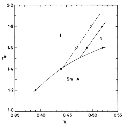
Figure 5: Phase diagram for the GB potential with parameters $x_{0}=4.4,k^{\prime}=20.0,\mu=1$ and $\nu$ = 1. The solid lines indicate the phase boundaries obtained by using the second-order density-functional theory. The dashed line demarcating the isotropic and nematic phase is found from the modified weighted density approximation version of the density-functional theory.

References

• (1) P.G. de Gennes and J. Prost, The Physics of Liquid Crystals (Clarendon, Oxford,1993); S.Chandrasekher, Liquid Crystals(Cambridge University Press,London,1977); Handbook of liquid crystal Research ed. by P.J. Collings and J.S. Patel (Oxford University Press, New York, 1997)
• (2) R. Pindak, D.E. Moncton, S.C. Davey and J.W. Goodby, Phys. Rev. Lett. 46, 1135 (1981)
• (3) J. G. Gay and B. J. Berne, J. Chem Phys. 74, 3316 (1981)
• (4) E.D.Miguel, L.F. Rull, M.K. Chalam and K.E. Gubbins, Mol. Phys. 74, 405(1991)
• (5) J.T.Brown, M.P.Allen and E. Martin del Rio, and E. de Miguel, Phys. Rev. E 57, 6685 (1998)
• (6) M.A. Bates and G.R. Luckhurst, J. Chem. Phys. 110, 7087(1999)
• (7) C.G. Gray and K.E. Gubbins, Theory of Molecular Fluids, Vol. 1(Clarendon, Oxford, 1984)
• (8) J. Ram and Y. Singh, Phys. Rev. A 44, 3718 (1991); J. Ram, R.C. Singh and Y. Singh, Phys. Rev. E 49, 5117(1994)
• (9) R.C. Singh, J.Ram and Y.Singh, Phys. Rev. E 54, 977 (1996)
• (10) R.C.Singh, J.Ram and Y. Singh, Phys. Rev. E 65, 031711 (2002)
• (11) Y.Singh, Phys.Rep. 207, 351 (1991)
• (12) A.R. Denton and N.W. Ashcroft, Phys. Rev. A 39, 426 (1989); 39, 4701 (1989)
Refer to caption