Short-range type critical behavior in spite of long-range interactions: the phase transition of a Coulomb system on a lattice

Abstract

One- to three-dimensional hypercubic lattices half-filled with localized particles interacting via the long-range Coulomb potential are investigated numerically. The temperature dependences of specific heat, mean staggered occupation, and of a generalized susceptibility indicate order-disorder phase transitions in two- and three-dimensional systems. The critical properties, clarified by finite-size scaling analysis, are consistent with those of the Ising model with short-range interaction.

The problem under which conditions Coulomb glasses exhibit genuine phase transitions has been under controversial debate for two decades DLR82 ; V93 ; GY93 ; VS94 ; Detal00 . The significance of the kind of static disorder is unclear yet GY93 ; VS94 . In this context, the relation to the Ising model with short-range interaction is of great interest. It would be very useful to know how replacing its nearest-neighbor coupling by an “antiferromagnetic” long-range Coulomb interaction modifies the critical behavior of a system without static disorder. Due to the interplay of long-range interaction and frustration, one might alternatively expect this model to belong to different universality classes: In case of a sufficiently slowly decaying ferromagnetic power-law interaction, including the $1/r$-interaction, mean field behavior is obtained LB02 . But the condensation in a three-dimensional model of an electrolyte exhibits Ising-like critical behavior, possibly due to efficient screening Letal02 .

To decide the question, we numerically study lattices half-filled with localized particles interacting via the long-range Coulomb potential,

$$H=\frac{1}{2}\sum_{i\neq j}\frac{(n_{i}-1/2)\,(n_{j}-1/2)}{\left|{\bf r}_{i}-{\bf r}_{j}\right|}\,\,.$$ (1)

Here $n_{\alpha}\in\{0,1\}$ denote the occupation numbers of states localized at sites ${\bf r}_{i}$ within a $d$-dimensional hypercube of size $L^{d}$. Elementary charge, lattice spacing, dielectric and Boltzmann constants are all taken to be 1. Neutrality is achieved by background charges -1/2 at each site.

For reducing finite-size effects, we impose periodic boundary conditions for $d=1$ and 2, using the minimum image convention Metro53 . For $d=3$, the same approach would give rise to an unphysical feature: The groundstate would be a layered arrangement of charges instead of the expected NaCl structure in case $L$ is a multiple of 4 Metal01 . Hence, for $d=3$, we consider the sample to be surrounded by eight equally occupied cubes.

Our numerical investigations have been performed by means of algorithms based on the Metropolis procedure Metro53 ; Metal01 ; MT97 . Such simulations are very expensive not only for the long-range interaction, but also for correlation times diverging close to phase transitions and as temperature $T$ vanishes. Therefore it is necessary to adapt the dynamics to the situation that the simultaneous change of $n_{i}$ for certain clusters is necessary for overcoming passes in the energy landscape. To our knowledge, a procedure similar to the Swendsen-Wang algorithm Swen.Wang is not available for the interaction type considered here. Hence we modified the dynamics “by hand” to take into account several kinds of processes: one-electron exchange with the surroundings, one-electron hops over ($T$ dependent) restricted distance, and two-electron hops simultaneously changing the occupation of four neighboring sites.

At high $T$, we use the original Metropolis method Metro53 . But at low $T$, we take advantage of a hybrid procedure much accelerating the computations. It connects the direct evaluation of weighted sums over states within a low-energy subset of the configuration space with Metropolis sampling of the complementary high-energy subset MT97 .

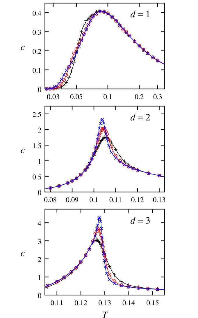
Figure 1: Temperature dependences of the specific heat, $c(T)$, for dimensions $d=1$ to 3 as obtained from simulations of samples of $L^{d}$ sites. $d=1$: $L=100$ ($+$), 280 ($\circ$), and 700 ($\times$); $d=2$: $L=20$ ($+$), 34 ($\circ$), and 58 ($\times$); $d=3$: $L=8$ ($+$), 12 ($\circ$), and 18 ($\times$). Only a part of the data points forming the curves is marked by symbols. The error bars are considerably smaller than the symbol size.

We now turn to the qualitative behavior of specific heat, order parameter, and susceptibility. The specific heat $c$ was obtained from energy fluctuations utilizing $c=(\langle H^{2}\rangle-\langle H\rangle^{2})/(T^{2}\ L^{d})\,$. The $T$ and $L$ dependences of $c$ are presented in Fig. 1 for dimensions $d=1$ to 3. This graph shows that, for $d=2$ and 3, sharp peaks of increasing height evolve within a small $T$ region as $L$ grows. Away from the peaks, within the $T$ intervals presented, $c$ is almost independent of $L$. But for $d=1$, there are only broad, rounded peaks with $L$ independent height – a logarithmic $T$ scale is used for $d=1$, in contrast to the linear scales for $d=2$ and 3 which display far smaller $T$ intervals. For $d=1$, finite size effects are restricted to low $T$ where the reliability bound decreases with $L$.

Hence, according to the behavior of $c(T,L)$ a phase transition likely occurs for $d=2$ and 3, in agreement with results of lattice gas simulations for $d=3$ Letal02 ; DS99 . However, for $d=1$, in spite of the long-range interaction, there seems to be no phase transition at finite $T$.

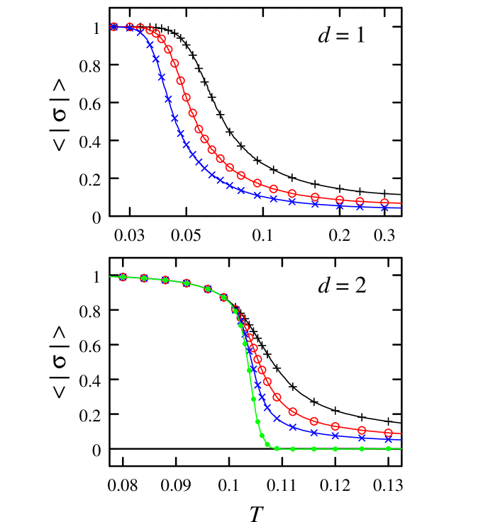
Figure 2: Temperature dependence of the mean absolute value of the staggered occupation, $\langle|\sigma|\rangle(T)$, for $d=1$ and 2. For the meaning of the symbols $+$, $\circ$, and $\times$ see caption of Fig. 1; $\bullet$ marks the extrapolation $L\rightarrow\infty$ explained in the text.

Analogously to an antiferromagnet, the order inherent in a charge arrangement $n_{i}$ can be characterized by means of the staggered occupation $\sigma_{i}$ relating to a NaCl structure. For example, if $d=3$, it is given by

$$\sigma_{i}=(2n_{i}-1)\cdot(-1)^{x_{i}+y_{i}+z_{i}}$$ (2)

where $x_{i}$, $y_{i}$, and $z_{i}$ denote the (integer) components of ${\bf r}_{i}$. Thus we measure the mean absolute value of the staggered occupation $\langle|\sigma|\rangle$ as order parameter.

$T$ and $L$ dependences of $\langle|\sigma|\rangle$ are shown in Fig. 2. For $d=1$, a rapid decrease of $\langle|\sigma|\rangle$ with increasing $T$ occurs already clearly below the temperature of maximum $c$ (same $T$ scales in Figs. 1 and 2). This marked decrease shifts to lower $T$ with increasing $L$. For $d=2$, a qualitatively different behavior is found: $\langle|\sigma|\rangle$ decreases rapidly just in that $T$ region where the peak of $c(T)$ evolves. The $T$ interval of rapidly diminishing $\langle|\sigma|\rangle$ shrinks as $L$ rises, another indication of the phase transition. This interpretation is confirmed by an extrapolation $L\rightarrow\infty$: Assuming $\langle|\sigma|\rangle(T,L)=\langle|\sigma|\rangle(T,\infty)+A(T)/L^{d/2}$ with $A$ independent of $L$, an almost sharp transition is obtained from data for $L=34$ and $58$, although this extrapolation is of limited accuracy in the immediate vicinity of the transition. For $d=3$, the results (not shown here) qualitatively resemble our findings for $d=2$.

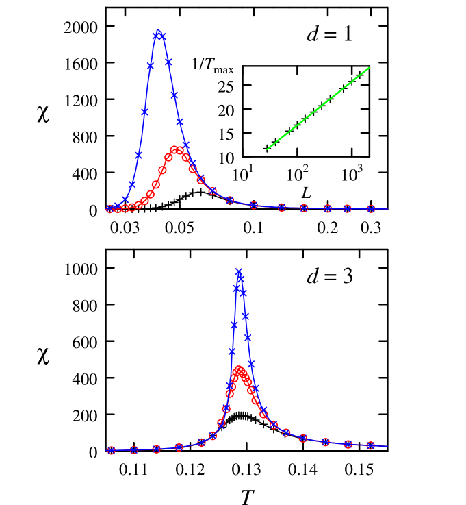
Figure 3: Temperature dependence of the susceptibility, $\chi(T)$, related to the staggered occupation $\sigma$ by Eq. (3), for $d=1$ and 3. For the meaning of the symbols see caption of Fig. 1. Additionally, for $d=1$, the inset shows how $T_{\rm{max}}$, the temperature of maximum $\chi(T)$, depends on sample size $L$.

The generalized susceptibility $\chi$ related to the order parameter $\langle|\sigma|\rangle$ is given by

$$\chi=L^{d}(\langle\sigma^{2}\rangle-\langle|\sigma|\rangle^{2})/T\ .$$ (3)

Fig. 3 shows $T$ and $L$ dependences of $\chi$. It confirms the conclusions drawn from $\langle|\sigma|\rangle(T,L)$: On the one hand, for $d=1$, a broad peak of $\chi(T)$ evolves with increasing $L$ where $T_{\rm{max}}$, the temperature of maximum $\chi$, decreases. As the inset demonstrates, $T_{\rm{max}}$ can be approximated by $a/\ln(b\,L)$ with constants $a$ and $b$. Hence, $T_{\rm{max}}$ likely vanishes as $L\rightarrow\infty$ so that there seems to be no phase transition for $d=1$ at finite $T$. On the other hand, for $d=3$, as $L$ rises, a narrow peak grows in just that $T$ region where $c(T,L)$ has such a feature, a further indication of the phase transition. For $d=2$, $\chi(T,L)$ behaves qualitatively similar to the results for $d=3$.

The quantitative evaluation of our simulation data consists in a finite-size scaling analysis Betal00 ; G92 . For this aim, we first consider $q_{2}=-\ln(1-\langle\sigma^{2}\rangle^{2}/\langle\sigma^{4}\rangle)$ and $q_{3}=-\tan(\pi\,(1-1.5\,\langle\sigma^{2}\rangle^{2}/\langle\sigma^{4}\rangle))$ for $d=2$ and 3, respectively. These quantities are directly derived from the Binder cumulant $1-\langle\sigma^{4}\rangle/(3\langle\sigma^{2}\rangle^{2})$ and exhibit similar features. The $q_{d}(T)$ have small curvature in the vicinity of the transition what alleviates a precise interpolation.

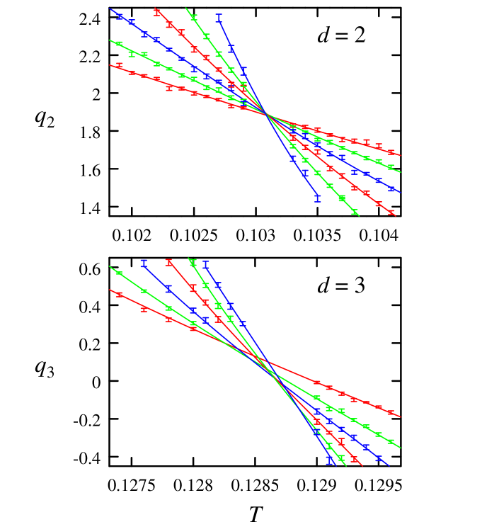
Figure 4: Temperature dependence of $q_{d}$, related to the Binder cumulant, in the close vicinity of the transition for $d=2$ and 3. For definitions see text. With increasing modulus of the slope, the curves refer to $L=16$, 24, 34, 48, 68, and 96 for $d=2$, and to $L=8$, 10, 12, 14, 16, and 18 for $d=3$. For clarity, data points in the intersection regions are omitted.

Fig. 4 shows $q_{d}(T)$. For $d=2$, there clearly is a common intersection point of the curves for different $L$ at the critical temperature $T_{{\rm c},2}$. But for $d=3$, only a tendency towards such a behavior is seen. However, the systematic corrections to scaling can to a large extent be taken into account in a simple way: We define a size-dependent critical temperature by $q_{d}(T_{{\rm c},d}(L),L)=q_{d,0}$ where the $q_{d,0}$ are appropriate constants, fixed below. Scaling of $q_{d}(T)$ curves for different $L$ with respect to $T-T_{{\rm c},d}(L)$ yields very good data collapse. (Referring to $t=0$ instead of $T=T_{{\rm c},d}(\infty)$ considerably reduces the influence of deviations from scaling on the values for the critical exponents Hase .) Thus we assume $q_{d}$ to depend only on $t=a_{d}(L)(T-T_{{\rm c},d}(L))$ in the vicinity of the transition.

We approximate $q_{d}(t)$ by polynomials of third degree, $q_{d,0}+t+b_{d}t^{2}+c_{d}t^{3}$. By regression studies we first adjusted the $L$ independent parameters $b_{d}$ and $c_{d}$ of the ansatz, and then determined the $a_{d}(L)$ values. The latter were analyzed by means of power law fits including various $L$ intervals, where according to finite-size scaling $a_{d}(L)\propto L^{1/\nu}$ was presumed. For consistency, the mean-square deviation of these fits must be understandable as resulting from random errors alone. Tab. I presents the most precise results for $\nu$, which were obtained from the fits safely fulfilling this requirement.

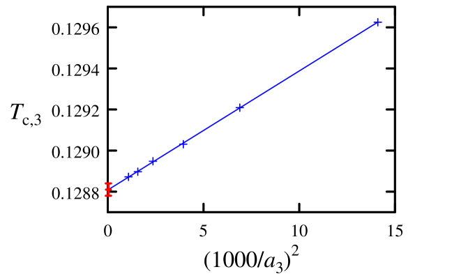
Figure 5: Relation between $a_{3}(L)$ and $T_{{\rm c},3}(L)$ for $q_{3,0}=-0.174$. With increasing $a_{3}$, the points refer to $L=8$, 10, 12, 14, 16, and 18. The error bar represents our extrapolation $L\rightarrow\infty$.

In obtaining $T_{{\rm c},d}(L)$ from $q_{d}(T_{{\rm c},d}(L),L)=q_{d,0}$, a deviation $\delta$ of $q_{d,0}$ from the $L\rightarrow\infty$ limit of $q_{d}(T,2L)=q_{d}(T,L)$ gives rise to a contribution $\propto\delta/a_{d}(L)$ to $T_{{\rm c},d}(L)$. We chose $q_{d,0}$ so that this term vanishes: $q_{2,0}=1.8933$ and $q_{3,0}=-0.174$. The remaining higher order corrections in $T_{{\rm c},d}(L)$ originate from imperfection of finite-size scaling. Comparing several empirical approximations, we observed that, over a wide $L$ range, they are almost proportional to $a_{d}(L)^{-2}$, see Fig. 5. Corresponding extrapolations yield the following values of $T_{{\rm c},d}(\infty)$: $0.10308\pm 0.00002$ and $0.12881\pm 0.00003$ for $d=2$ and 3, respectively. The confidence intervals include the $3\sigma$-random errors and cautious estimates for the systematic uncertainty of the extrapolation $L\rightarrow\infty$, see Fig. 5.

The analysis of $c(T,L)$, $\langle|\sigma|\rangle(T,L)$, and $\chi(T,L)$ was performed similarly to the evaluation of $q_{d}(T,L)$: We considered $\ln c$, $\ln\langle|\sigma|\rangle$, and $\ln\chi$ as functions of $t$ and $L$. For not too large $|t|$, as $L\rightarrow\infty$, scaling implies that each of these quantities is decomposable into a sum of two functions depending only on $t$ and $L$, respectively. However, for the $L$ regions considered here, this hypothesis proved to be well fulfilled only for $\ln\chi$. In the cases of $\ln c$ and $\ln\sigma$, there is a clear tendency towards such a behavior, but small deviations cannot be neglected. Thus we approximated $\ln c$, $\ln\langle|\sigma|\rangle$, and $\ln\chi$ by polynomials in $t$ of third order, taking advantage of universalities in the coefficients as far as possible. This regression provides precise values for the observables at $t=0$. Simultaneously, we obtained the confidence intervals taking into account the uncertainties in the individual measurements of the observables and in the $T_{{\rm c},d}(L)$ values.

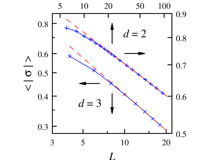
Figure 6: Size dependence of the value of $\langle|\sigma|\rangle$ at $T_{{\rm c},d}(L)$ defined in the text. Error bars are considerably smaller than symbol size. The dashed lines represent the fits given in Tab. I.

The interpolation results for $\langle|\sigma|\rangle$ and $\chi$ were analyzed by means of power law fits, where proportionality to $L^{-\beta/\nu}$ and $L^{\gamma/\nu}$, respectively, was presumed. These studies were performed analogously to the determination of $\nu$. Tab. I presents the values of the exponent ratios $\beta/\nu$ and $\gamma/\nu$. The high quality of these power law fits is illustrated by Fig. 6 presenting $\langle|\sigma|\rangle(T_{\rm c}(L),L)$.

Quantity	$d$	$L$ region	Coulomb	s.-r. Ising
$\alpha/\nu$	2	24 – 96	-0.037(44)	0 (ln)
$\beta/\nu$	2	48 – 96	0.131(6)	1/8
$\gamma/\nu$	2	48 – 96	1.735(24)	7/4
$\nu$	2	34 – 96	1.021(33)	1
$\alpha/\nu$	3	6 – 18	0.09(6)	0.1761[25]
$\beta/\nu$	3	12 – 18	0.499(16)	0.5181[4]
$\gamma/\nu$	3	14 – 18	1.974(23)	1.9638[8]
$\nu$	3	10 – 18	0.635(10)	0.6297[5]

Table 1: Finite-size scaling results for the critical exponents of specific heat, staggered occupation, susceptibility, and correlation length, $\alpha$, $\beta$, $\gamma$, and $\nu$, respectively. To retain numerical precision, we mostly present exponent ratios instead of the exponents themselves. Values for the Ising model with short-range interaction G92 ; Hase are included for comparison. Parentheses and brackets give $3\sigma$-random errors and total errors, respectively, referring to the last given digit of the value.

Compared to the study of $\langle|\sigma|\rangle$ and $\chi$, the analysis of $c$ is more difficult: Exponent values obtained from power law fits converge only slowly with increasing $L$, and the mean-square deviations remain too large. Therefore we took into account a background contribution presuming $c(T_{\rm c}(L),L)=f(L)=a+bL^{\alpha/\nu}$. However, we treated $f(L_{1})$ and $f(L_{2})$ at fixed finite $L_{1}$ and $L_{2}$ as adjustable parameters instead of $a$ and $b$ to avoid numerical problems for almost logarithmic behavior of $c(L)$ (small $|\alpha|$). Results for $\alpha/\nu$ obtained this way are included in Tab. I.

Our values in Tab. I have to be regarded as effective exponents. Due to the finiteness of $L$, tiny systematic errors are certainly present, presumably the more relevant the smaller the exponent value. Unfortunately, our data set is not sufficient for a convincing estimate of them. However, even if only random errors are considered, our values comply with the Widom relation, $2=\alpha+2\beta+\gamma$, and the hyperscaling relation, $2-\alpha=d\,\nu$.

For comparison, Tab. I includes also values for the Ising model with nearest-neighbor interaction G92 ; Hase . It is surprising that, in spite of the differing characters of the interactions, the critical exponent data obtained here are very close to these values: In particular, for $\gamma/\nu$ and $\nu$. the agreement is perfect within numerical accuracy. The slight deviations in $\alpha/\nu$ and $\beta/\nu$ for $d=3$ presumably arise from a too small sample size. Note: obtaining these values indirectly, via Widom and hyperscaling relation from $\gamma/\nu$ and $\nu$, yields again perfect agreement.

Concluding, in spite of the long-range interaction, the Coulomb system described by Eq. (1) seems to belong to the same universality class as the Ising model with short-range interaction. This suggests that the lattice Coulomb-glass model might have the same critical properties as the random-field short-range Ising model.

- (1) J.H. Davies, P.A. Lee, and T.M. Rice, Phys. Rev. Lett. 49, 758 (1982).
- (2) T. Vojta, J. Phys. A: Math. Gen. 26, 2883 (1993).
- (3) E.R. Grannan, C.C. Yu, Phys. Rev. Lett. 71, 3335 (1993).
- (4) T. Vojta, M. Schreiber, Phys. Rev. Lett. 73, 2933 (1994).
- (5) A. Díaz-Sánchez, M. Ortuño, A. Pérez-Garrido, E. Cuevas, phys. stat. sol. (b) 218, 11 (2000).
- (6) E. Luijten and W.J. Blöte, Phys. Rev. Lett. 89, 025703-1 (2002), and refs. therein.
- (7) E. Luijten, M.E. Fisher, and A.Z. Panagiotopoulos, Phys. Rev. Lett. 88, 184701-1 (2002).
- (8) N. Metropolis, A.W. Rosenbluth, M.N. Rosenbluth, A.H. Teller, E. Teller, J. Chem. Phys. 21, 1087 (1953).
- (9) A. Möbius, P. Thomas, J. Talamantes, and C.J. Adkins, Phil. Mag. B 81, 1105 (2001).
- (10) A. Möbius, P. Thomas, Phys. Rev. B 55, 7460 (1997).
- (11) R.H. Swendsen and J.S. Wang, Phys. Rev. Lett. 58, 86 (1987).
- (12) R. Dickman and G. Stell, cond-mat/9906364.
- (13) K. Binder, E. Luijten, M. Müller, N.B. Wilding, and H.W.J. Blöte, Physica A 281, 112 (2000), and refs. therein.
- (14) N. Goldenfeld, Lectures on Phase Transitions and the Renormalization Group, Frontiers in Physics, Vol. 85, (Wesley, Reading, 1992).
- (15) M. Hasenbusch, Int. J. Mod. Phys. C 12, 911 (2001).