How to calculate the main characteristics
of random graphs - a new approach

Abstract

The poster presents an analytic formalism describing metric properties of undirected random graphs with arbitrary degree distributions and statistically uncorrelated (i.e. randomly connected) vertices. The formalism allows to calculate the main network characteristics like: the position of the phase transition at which a giant component first forms, the mean component size below the phase transition, the size of the giant component and the average path length above the phase transition. Although most of the enumerated properties were previously calculated by means of generating functions, we think that our derivations are conceptually much simpler.

A poster presented at Midterm Conference COSIN -
Conference on Growing Networks and Graphs
in Statistical Physics, Finance, Biology and Social Systems,
Roma 1-5 September 2003.

1 Introduction

Let us start with the following lemma.

Lemma 1

If $A_{1},A_{2},\dots,A_{n}$ are mutually independent events and their probabilities fulfill relations $\forall_{i}P(A_{i})\leq\varepsilon$ then

$$P(\bigcup_{i=1}^{n}A_{i})=1-\exp(-\sum_{i=1}^{n}P(A_{i}))-q,$$ (1)

where $q<\sum_{j=0}^{n+1}(n\varepsilon)^{j}/j!-(1+\varepsilon)^{n}$ and may be neglected in the limit of large $n$.

The complete proof of the Lemma is given in [1]. In the course of the presentation, we will take advantage of the Lemma several times.

A random graph with a given degree distribution $P(k)$ is the simplest network model [2]. In such a network the total number of vertices $N$ is fixed. Degrees of all vertices are independent, identically distributed random integers drawn from a specified distribution $P(k)$ and there are no vertex-vertex correlations. Because of the lack of correlations the probability that there exists a walk of length $x$ crossing index-linked vertices $\{i,v_{1},v_{2}\dots v_{(x-1)},j\}$ is described by the product $\widetilde{p}_{iv_{1}}\;\widetilde{p}_{v_{1}v_{2}|iv_{1}}\;\widetilde{p}_{v_{2}v_{3}|v_{1}v_{2}}\dots\widetilde{p}_{v_{(x-1)}j|v_{(x-2)}v_{(x-1)}}$, where

$$\widetilde{p}_{ij}=\frac{k_{i}k_{j}}{\langle k\rangle N}$$ (2)

gives a connection probability between vertices $i$ and $j$ with degrees $k_{i}$ and $k_{j}$ respectively, whereas

$$\widetilde{p}_{ij|li}=\frac{(k_{i}-1)k_{j}}{\langle k\rangle N}$$ (3)

describes the conditional probability of a link $\{i,j\}$ given that there exists another link $\{l,i\}$. Taking advantage of the Lemma 1 one can write the probability $p_{ij}^{+}(x)$ of at least one walk of length $x$ between $i$ and $j$

$$p_{ij}^{+}(x)=1-\exp[-\sum_{v_{1}=1}^{N}\sum_{v_{2}=1}^{N}\dots\sum_{v_{(x-1)}=1}^{N}\widetilde{p}_{iv_{1}}\dots\widetilde{p}_{v_{(x-1)}j|v_{(x-2)}v_{(x-1)}}].$$ (4)

Putting (2) and (3) into (4) and replacing the summing over nodes indexes by the summing over the degree distribution $P(k)$ one gets:

$$p_{ij}^{+}(x)=1-\exp\left[-\frac{k_{i}k_{j}}{N}\frac{\langle k(k-1)\rangle^{x-1}}{\langle k\rangle^{x}}\right].$$ (5)

2 Random graphs below the percolation
threshold - the mean component size

According to (5), the probability that none among the walks of length $x$ between $i$ and $j$ occurs is given by

$$p_{ij}^{-}(x)=1-p_{ij}^{+}(x)=\exp\left[-\frac{k_{i}k_{j}}{N}\frac{\langle k(k-1)\rangle^{x-1}}{\langle k\rangle^{x}}\right]$$ (6)

and respectively the probability that there is no walk of any length between these vertices may be written as

$$p_{ij}^{-}=\prod_{x=1}^{\infty}\;p_{ij}^{-}(x)=\prod_{x=1}^{\infty}\;\exp\left[-\frac{k_{i}k_{j}}{N}\frac{\langle k(k-1)\rangle^{x-1}}{\langle k\rangle^{x}}\right]\;=\;$$

$$=\;\exp\left[-\;\frac{k_{i}k_{j}}{\langle k\rangle N}\;\sum_{y=0}^{\infty}\;\left(\frac{\langle k^{2}\rangle}{\langle k\rangle}-1\right)^{y}\right].$$ (7)

The value of $\;p_{ij}^{-}\;$ strongly depends on the common ratio of the geometric series present in the last equation. When the common ratio is greater then $1$ i.e. $\langle k^{2}\rangle\geq 2\langle k\rangle$ random graphs are above the percolation threshold. The sum of the geometric series in (2) tends to infinity and $p_{ij}^{-}=0$. Below the phase transition, when $\langle k^{2}\rangle<2\langle k\rangle$, the probability that the nodes $i$ and $j$ belong to separate clusters is given by

$$p_{ij}^{-}\;=\;\exp\left[-\;\frac{k_{i}k_{j}}{N}\frac{1}{(2\langle k\rangle-\langle k^{2}\rangle)}\right]$$ (8)

and respectively the probability that $i$ and $j$ belong to the same cluster may be written as

$$p_{ij}^{+}\;=\;1-p_{ij}^{-}\;=\;1-\exp\left[-\;\frac{k_{i}k_{j}}{N}\frac{1}{(2\langle k\rangle-\langle k^{2}\rangle)}\right].$$ (9)

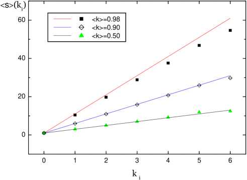
Figure 1: Average size of the component that a node $i$ with degree $k_{i}$ belongs to. Scatter plots represent numerical data, whereas solid lines represent the prediction of Eq. (10).

Now, it is simple to calculate the mean size of the cluster that the node $i$ belongs to. It is given by

$$\langle s\rangle(k_{i})\;=\;\sum_{k_{j}}P(k_{j})p_{ij}^{+}+1\;\simeq\;\frac{\langle k\rangle}{2\langle k\rangle-\langle k^{2}\rangle}k_{i}+1.$$ (10)

Note, that the mean size of the component that a node $i$ belongs to, is proportional to degree $k_{i}$ of the node (see Fig. 1). The last transformation in (10) was obtained by taking only the first two terms of power series expansion of the exponential function in (9). Averaging the above expression (10) over all nodes in the network one obtains the well-known formula [2] for the mean component size in random graphs below the phase transition

$$\langle s\rangle\;=\;1+\frac{\langle k\rangle^{2}}{2\langle k\rangle-\langle k^{2}\rangle}.$$ (11)

As in percolation theory [7], the mean cluster size diverges at

$$\langle k^{2}\rangle=2\langle k\rangle,$$ (12)

signifying that the expression (12) describes the position of the percolation threshold in random graphs with arbitrary degree distributions [2, 3, 4].

3 Random graphs above the percolation
threshold - the size of the giant component

When $\langle k^{2}\rangle>2\langle k\rangle$ the giant component (GC) is present in the graph. The size of the giant component $N_{GC}$ scales as the size of the graph as a whole $N$. Its relative size $S=N_{GC}/N$ (i.e. the probability that a node belongs to GC) is an important quantity in percolation theory and is often identified as the order parameter. Here we demonstrate how to calculate the size of the giant component in undirected random graphs. The underlying concept, how to calculate $S$, is closely related to the method of calculating $S$ in Cayley tree presented in [7].

At the beginning, we deal with classical random graphs of Erdös and Rényi, then we generalize our derivations for the case of random graphs with arbitrary degree distributions and we show that our derivations are consistent with the formalism based on generating functions that was introduced by Newman et al. [2].

3.1 The giant component in classical random graphs
of Erdös and Rényi

In general terms, classical random graphs consist of a fixed number of vertices $N$, which are connected at random with a fixed probability $p$ [5].

Let us call $R$ the probability that an arbitrary node $i$ is connected to the giant component through a fixed link $\{i,j\}$, where $j$ is another arbitrary node. Since every node in the graph may have $N-1\simeq N$ links and all nodes are equivalent, the formula for $R$ may be written as the product of the probability of a link $\{i,j\}$ and the probability that at least one of $N$ possible links emanating from $j$ connects $j$ to the giant component. Taking advantage of the Lemma 1 one can write

$$R\;=\;p\;(1-\exp[-RN]).$$ (13)

This self-consistency equation for $R$ has one or two solutions, depending on whether a graph is below ($pN<1$) or above ($pN>1$) the phase transition. Graphical solution of the equation (13) shown at Fig. 2 presents the easiest way to obtain a qualitative understanding of percolation transition in classical random graphs.

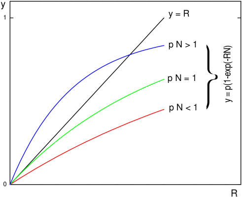
Figure 2: Graphical solution of the equation (13).

The probability that an arbitrary node $i$ belongs to the giant component is equivalent to the probability that at least one of $N$ possible links connects $i$ to GC. Again, taking advantage of the Lemma 1. one gets

$$S\;=\;1-\exp[-RN].$$ (14)

Comparing both relations (13) and (14) it is easy to see that $R=pS$ and the expression (14) for the giant component in classical random graphs may be rewritten in the form

$$S\;=\;1-\exp[-\langle k\rangle S],$$ (15)

where $\langle k\rangle=pN$. Fig. 3 presents the prediction of the Eq. (15) in comparison with numerically calculated sizes of the giant components in classical random graphs.

It is necessary to stress that both equations (13) and (14) are well-known and have been independently derived using different methods by Newman et al. [2] and Molloy and Reed [6].

3.2 The giant component in random graphs
with arbitrary degree distributions $P(k)$

In the case of classical random graphs all vertices have been considered as equivalent. It is not acceptable in the case of random graphs with a given degree distribution $P(k)$, where each node $i$ is characterized by its degree $k_{i}$.

Here, we call $R^{*}$ the probability that following arbitrary direction of a randomly chosen edge we arrive at the giant component. In fact, we know that following an arbitrary edge we arrive at a vertex $i$ with degree $k_{i}$. The probability that $i$ is connected to GC is $1-(1-R^{*})^{k_{i}-1}$. The notation expresses the probability that at least one of $k_{i}-1$ edges emanating from $i$ and other than the edge we arrived along connects $i$ to the giant component. Now, it is simple to write the self-consistency condition for $R^{*}$

$$R^{*}\;=\;\sum_{k_{i}}\left(1-(1-R^{*})^{k_{i}-1}\right)Q(k_{i}),$$ (16)

where $Q(k_{i})=k_{i}P(k_{i})/\langle k\rangle$ describes the probability that an arbitrary link leads to a node $i$ with degree $k_{i}$. As in the case of classical random graphs the equation (16) can be solved graphically, signifying that the nontrivial solution (i.e. $R^{*}\neq 0$) of the equation (16) exists only for random graphs above the percolation threshold $\langle k^{2}\rangle>2\langle k\rangle$.

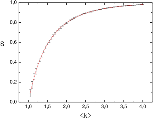
Figure 3: The size of the giant component $S$ versus the mean node degree $\langle k\rangle$ in classical random graphs of size $N=10000$. The scatter plot represents numerical data whereas the solid line gives the solution of the Eq.(15)

.

Knowing $R^{*}$, it is simple to calculate the relative size $S$ of the giant component in random graphs with arbitrary degree distribution $P(k)$. $S$ is equivalent to the probability that at least one of $k$ links attached to an arbitrary node connects the node to the giant component

$$S\;=\;\sum_{k}\left(1-(1-R^{*})^{k}\right)P(k).$$ (17)

It is easy to show that both equations (17) and (16) are completely equivalent to equations derived by Newman et al. by means of generating functions

$$S=1-G_{0}(v),$$ (18)

where $v$ is the solution of equation given below

$$v=G_{1}(v).$$ (19)

We recall that $G_{0}(x)$ is the generating function for the probability distribution of vertex degrees

$$G_{0}(x)=\sum_{k}P(k)x^{k},$$ (20)

whereas $G_{1}(x)$ is given by

$$G_{1}(x)=\frac{G^{{}^{\prime}}_{0}(x)}{\langle k\rangle}=\frac{1}{\langle k\rangle}\sum_{k}kP(k)x^{k-1}.$$ (21)

At the beginning we show that Eq. (16) is completely equivalent to Eq. (19). Expression (16) may be transformed in the following way

$$R^{*}=\frac{1}{\langle k\rangle}\sum_{k}kP(k)-\frac{1}{\langle k\rangle}\sum_{k}kP(k)(1-R^{*})^{k-1}=1-G_{1}(1-R^{*}),$$

that exactly corresponds to Eq. (19) with $v=1-R^{*}$. Expression (17) may be transformed into Eq. (18) in a similar way, when assume that $v=1-R^{*}$. Now, it is clear that the unknown parameter $v$ in both Eqs. (18) and (19) has the following meaning:

$$v=1-R^{*}$$ (22)

describes the probability that an arbitrary edge in random graph does not belong to the giant component.

4 Average path length in random graphs

This part of the presentation closely follows that of Fronczak et al. [1].

Let us consider the situation when there exists at least one walk of the length $x$ between the vertices $i$ and $j$. If the walk(s) is(are) the shortest path(s) $i$ and $j$ are exactly $x$-th neighbors otherwise they are closer neighbors. In terms of statistical ensemble of random graphs the probability $p_{ij}^{+}(x)$ (Eq. (5)) of at least one walk of the length $x$ between $i$ and $j$ expresses also the probability that these nodes are neighbors of order not higher than $x$. Thus, the probability that $i$ and $j$ are exactly $x$-th neighbors is given by the difference

$$p_{ij}^{*}(x)=p_{ij}^{+}(x)-p_{ij}^{+}(x-1).$$ (23)

Due to (5) the probability that both vertices are exactly the $x$-th neighbors may be written as

$$p_{ij}^{*}(x)=F(x-1)-F(x),$$ (24)

where

$$F(x)=\exp\left[-\frac{k_{i}k_{j}}{N}\frac{(\langle k^{2}\rangle-\langle k\rangle)^{x-1}}{\langle k\rangle^{x}}\right].$$ (25)

Now, it is simple to calculate the average path length (APL) between $i$ and $j$. It is given by

$$l_{ij}(k_{i},k_{j})=\sum_{x=1}^{\infty}\>x\>p_{ij}^{*}(x)=\sum_{x=0}^{\infty}F(x).$$ (26)

Notice that a walk may cross the same node several times thus the largest possible walk length can be $x=\infty$.

The Poisson summation formula

$$\sum_{x=0}^{\infty}F(x)=\frac{1}{2}F(0)+\int_{0}^{\infty}F(x)dx+2\sum_{n=1}^{\infty}\left(\int_{0}^{\infty}F(x)\cos(2n\pi x)dx\right)$$ (27)

allows us to simplify (26). Firstly, let us note that in most of real networks $\langle k\rangle\ll N$ thus we can assume

$$\frac{k_{i}k_{j}}{N\langle k^{2}\rangle}\simeq 0$$ (28)

that gives $F(0)=1$. Secondly, we have

$$\int_{0}^{\infty}F(x)dx=-Ei\left(-\frac{k_{i}k_{j}}{\langle k^{2}\rangle N}\right)/\ln\left(\frac{\langle k^{2}\rangle}{\langle k\rangle}\right),$$ (29)

where $Ei(y)$ is the exponential integral function that for negative arguments is given by $Ei(-y)=\gamma+\ln y+\int_{0}^{y}(\exp(-t)-1)/t\>dt$ [11], where $\gamma\simeq 0.5772$ is the Euler’s constant. Due to (28) the integral in the expression for $Ei(-y)$ becomes zero. Finally, every integral in the last term of the summation formula (27) is equal to zero owing to the generalized mean value theorem [12]. It follows that the equation for the APL between $i$ and $j$ may be written as

$$l_{ij}(k_{i},k_{j})=\frac{-\ln k_{i}k_{j}+\ln(\langle k^{2}\rangle-\langle k\rangle)+\ln N-\gamma}{\ln(\langle k^{2}\rangle/\langle k\rangle-1)}+\frac{1}{2}.$$ (30)

The average intervertex distance for the whole network depends on a specified degree distribution $P(k)$

$$l=\frac{\ln(\langle k^{2}\rangle-\langle k\rangle)-2\langle\ln k\rangle+\ln N-\gamma}{\ln(\langle k^{2}\rangle/\langle k\rangle-1)}+\frac{1}{2}.$$ (31)

A similar result $l\sim\ln N/\ln(\langle k^{2}\rangle/\langle k\rangle-1)$ was obtained by Dorogovtsev et al. [8]. The formulas (30) and (31) diverge when $\langle k^{2}\rangle=2\langle k\rangle$, giving the well-known expression for percolation threshold in undirected random graphs (12).

4.1 Average path length in classical random graphs
of Erdös and Rényi

For these networks the degree distribution is given by the Poisson function $P(k)=e^{-\langle k\rangle}\langle k\rangle^{k}/k!$. However, since $\langle\ln k\rangle$ cannot be calculated analytically for Poisson distribution thus the $APL$ may not be directly obtained from (31). To overcome this problem we take advantage of the mean field approximation. Let us assume that all vertices within a graph possess the same degree $\forall_{i}\>k_{i}=\langle k\rangle$. It implies that the $APL$ between two arbitrary nodes $i$ and $j$ (31) should describe the average intervertex distance of the whole network

$$l_{ER}=\frac{\ln N-\gamma}{\ln(pN)}+\frac{1}{2}.$$ (32)

Until now only a rough estimation of the quantity has been known. One has expected that the average shortest path length of the whole ER graph scales with the number of nodes in the same way as the network diameter. We remind that the diameter $d$ of a graph is defined as the maximal distance between any pair of vertices and $d_{ER}=\ln N/\ln(pN)$. Fig.4 shows the prediction of the equation (32) in comparison with the numerically calculated $APL$ in classical random graphs.

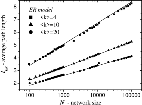
Figure 4: The average path length $l_{ER}$ versus network size $N$ in $ER$ classical random graphs with $\langle k\rangle=pN=4,10,20$. Solid curves represent numerical prediction of Eq.(32).

4.2 Average path length in scale-free
Barabási-Albert networks

The basis of the $BA$ model is its construction procedure. Two important ingredients of the procedure are: continuous network growth and preferential attachment. The network starts to grow from an initial cluster of $m$ fully connected vertices. Each new node that is added to the network creates $m$ links that connect it to previously added nodes. The preferential attachment means that the probability of a new link growing out of a vertex $i$ and ending up in a vertex $j$ is given by $\widetilde{p}_{ij}^{BA}=mk_{j}(t_{i})/\sum_{l}k_{l}(t_{i})$, where $k_{j}(t_{i})$ [9] denotes the connectivity of a node $j$ at the time when a new node $i$ is added to the network. Taking into account the time evolution of node degrees in $BA$ networks one can show that the probability $\widetilde{p}_{ij}^{BA}$ is equivalent to (2). Now let us consider the conditional probability $\widetilde{p}_{ij|li}$. Checking the possible time order of the vertices $i,j,l$ it is easy to see that in five of $3!$ cases $\widetilde{p}_{ij|li}=\widetilde{p}_{ij}$ and in a good approximation we get instead of (5) the result

$$p_{ij}^{+}(x)=1-\exp\left[-\frac{k_{i}k_{j}}{N}\frac{\langle k^{2}\rangle^{x-1}}{\langle k\rangle^{x}}\right].$$ (33)

It was found [9] that the degree distribution in $BA$ network is given by $P(k)=2m^{2}k^{-\alpha}$, where $k=m,m+1,\dots,m\sqrt{N}$, and the scaling exponent $\alpha=3$. Putting $\langle k\rangle=2m$, $\langle k^{2}\rangle=m^{2}\ln N$ and taking into account (33) one gets that the $APL$ between $i$ and $j$ is given by

$$l_{ij}^{BA}(k_{i},k_{j})=\frac{-\ln(k_{i}k_{j})+\ln N+\ln(2m)-\gamma}{\ln\ln N+\ln(m/2)}+\frac{3}{2}.$$ (34)

Averaging (34) over all vertices we obtain

$$l_{BA}=\frac{\ln N-\ln(m/2)-1-\gamma}{\ln\ln N+\ln(m/2)}+\frac{3}{2}.$$ (35)

Fig.5 shows the $APL$ of $BA$ networks as a function of the network size $N$ compared with the analytical formula (35). There is a visible discrepancy between the theory and numerical results when $\langle k\rangle=4$. The discrepancy disappears when the network becomes denser i.e. when $\langle k\rangle$ increases.

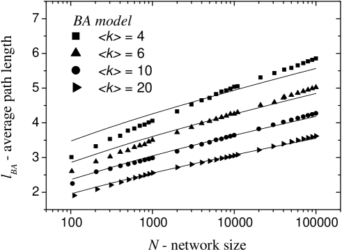
Figure 5: Characteristic path length $l_{BA}$ versus network size $N$ in $BA$ networks. Solid lines represent Eq.(35).

4.3 Average path length in scale-free networks
with arbitrary scaling exponent

Let us consider scale-free random graphs with degree distribution given by a power law, i.e. $P_{\alpha}(k)=(\alpha-1)m^{\alpha-1}k^{-\alpha}$, where $k=m,m+1,\dots,mN^{1/(\alpha-1)}$ [10]. Taking advantage of (31) we get that for large networks $N\gg 1$ the $APL$ scales as follows

• $l\simeq 2/(3-\alpha)+1/2\>\>\>$ for $2<\alpha<3$,

• $l\simeq\ln N/\ln\ln N+3/2\>\>\>$ for $\alpha=3$,

• $l\simeq\ln N/(\ln(m(\alpha-2)/(\alpha-3)-1)+1/2\>\>\>$ for $\alpha>3$.

The result for $\alpha\geq 3$ is consistent with estimations obtained by Cohen and Havlin [10]. The first case with $l$ independent on $N$ shows that there is a saturation effect for the mean path length in large scale-free networks with scaling exponent from the range $2<\alpha<3$. Our derivations show that the behaviour of $APL$ within scale-free networks is even more intriguring than reported by Cohen and Havlin [10].

References

- [1] A. Fronczak, P. Fronczak and J.A. Hołyst, Average path length in random networks, cond-mat/0212230.
- [2] M.E.J. Newman, S.H. Strogatz and D.J. Watts, Random graphs with arbitrary degree distributions and their applications,Phys. Rev. E 64, 026118 (2001).
- [3] M. Molloy and B. Reed, A critical point for random graphs with a given degree sequence, Random Struct. Algorithms 6, 161 (1995).
- [4] R. Cohen, K. Erez, D. ben-Avraham and S. Havlin, Resilience of the Internet to random breakdowns, Phys. Rev. Lett. 85 4626 (2000).
- [5] B. Bollobás, Random graphs, Academic Press, New York (1985).
- [6] M. Molloy and B.Reed, The size of the giant component of a random graph with a given degree sequence, Combinatorics, Probab. Comput. 7, 295 (1998).
- [7] D. Stauffer and A. Aharony, Introduction to Percolation Theory, Taylor and Francis, London (1994).
- [8] S.N.Dorogovtsev, J.F.F. Mendes and A.N. Samukhin., Metric structure of random networks, Nucl. Phys. B 653 307 (2003).
- [9] A.L. Barabási, R. Albert and H.Jeong, Mean-field theory for scale-free random networks, Physica A 272 173 (1999).
- [10] R. Cohen and S. Havlin, Scale-free networks are ultrasmall, Phys. Rev. Lett. 90 058701 (2003).
- [11] I.S. Gradshteyn et al., Table of Integrals, Series, and Products, Academic Press (2000).
- [12] G.M. Fichtenholz, Differential and integral calculus vol.2 (in Polish), PWN (1995).