A Simultaneous Magneto-Dielectric Phase Transition in RbCoBr₃

Abstract

We have modeled magneto-dielectric phase transitions in ABX₃-type layered triangular lattice compounds. The model consists of a spin system (magnetic transition) and a lattice system (dielectric transition). Magnetic exchange interactions are supposed to change with a relative position between two spins. This assumption produces an effective coupling between the lattice and the spin. Applying the nonequilibrium relaxation method, we have found that a simultaneous magneto-dielectric phase transition occurs when energy scales of the spin part and the lattice part coincide. An intermediate phase like the partial disordered phase disappears. Both systems relax frustration of the other system cooperatively and realize ordered states.

1 Introduction

The ABX₃-type layered triangular lattice antiferromagnets have been attracting great interests both experimentally and theoretically. [1, 2, 3, 4, 5, 6, 7, 8, 9, 10, 11, 12, 13] As the typical compounds we may list CsNiCl₃, CsCoCl₃, RbMnBr₃, KNiCl₃ and RbCoBr₃. The crystal structure is hexagonal close packed. Face-sharing BX₆ octahedra run along the $c$-axis forming a BX₃ chain. Magnetic B²⁺ ions form an equilateral triangular lattice on the $c$-plane. It causes frustration in the exchange interactions. Exchange interactions along the BX₃ chains are much stronger than those on the plane. This spin system can be considered as a quasi-one-dimensional system with frustration on the $c$-plane.

Successive magnetic phase transitions occur in the Ising antiferromagnet on the two-dimensional triangular lattice with ferromagnetic next-nearest-neighbor interactions. [2, 5, 6]. A low-temperature magnetic structure is the ferrimagnetic state (we abbreviate it with “Ferri” hereafter). There exists a partially-disordered (PD) phase between the paramagnetic (Para) phase and the ferrimagnetic phase. One of three sublattices is completely disordered in this phase. The other sublattices take antiferromagnetic configurations. The PD phase is also considered to exist in the layered three-dimensional model.[4, 5, 7, 9, 10] Since no anomaly of the specific heat was observed in the experiment [8] between the ferrimagnetic phase and the PD phase, there is a possibility that this change of the magnetic structure is a crossover between the PD-like state and the ferrimagnetic-like state. [10]

A typical lattice structure of the ABX₃-type compounds at high temperatures is shown in Fig. 1 (a). The space group is $P6_{3}/mmc$. The structure is sometimes referred to as a CsNiCl₃-type. Magnetic ions forming an equilateral triangular lattice sit on a level plane ($c$-plane). We call this structure “lattice Para” in this paper because it is a symmetric structure at high temperatures like the paramagnetic state. When the temperature is lowered, structural phase transitions occur. Each BX₃ chain shifts upward or downward keeping the relative distance between atoms in a chain unchanged. Some compounds take a structure in which two of three sublattices on the triangular lattice shift upward while the other one shifts downward as shown in Fig. 1 (b). The space group is $P6_{3}cm$. It is a room temperature structure of KNiCl₃. Since the displacement is $\uparrow$-$\uparrow$-$\downarrow$ type, we refer to this structure as “lattice Ferri” in this paper. Other compounds take a structure with one sublattice shifting upward, one shifting downward and the rest unchanged as shown in Fig. 1 (c). The space group is $P\bar{3}c1$. We refer to this structure as “lattice PD” since the displacement is $\uparrow$-$\downarrow$-0.

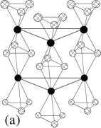
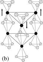
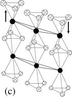
Figure 1: Typical crystal structures in ABX₃-type compounds. Solid circles depict magnetic B²⁺ ions and open circles depict X^- ions. (a) A symmetric structure at high temperatures. The space group is $P6_{c}/mmc$. We call this structure “lattice Para” in this paper. (b) A room-temperature KNiCl₃ structure. The space group is $P6_{3}cm$. We call this structure “lattice Ferri”. (c) Another low temperature structure. The space group is $P\bar{3}c1$. We call this structure “lattice PD”.

It is known that each BX₃ chain possesses negative charge. When a structural phase transition occurs, it can be observed by dielectric polarization. For example, a structure of the room-temperature KNiCl₃ family (Fig. 1 (b)) induces macroscopic polarization. This is a distinct difference compared with the other structures in Fig. 1. Morishita et al. [12] classified structural phase transitions in ABX₃-type compounds by the polarization observation. A structural phase transition and a magnetic phase transition occur at different temperatures. A structural phase transition usually occurs at a higher temperature. This is because an energy scale of the lattice system is larger than that of the spin system. A lattice changes its structure from the symmetric one to a distorted one. A magnetic state remains paramagnetic. When the temperature is lowered, a magnetic phase transition occurs from the paramagnetic state to the PD state or to the ferrimagnetic state.

Recently, Morishita et al. found that a structural phase transition and a magnetic phase transition occur at the same temperature in RbCoBr₃. [13] The magnetic susceptibility shows a peak at 37K, which suggests that a magnetically ordered state is realized at lower temperatures. The magnetic state has not been identified. The structural phase transition is observed at the same temperature by a peak of the dielectric constant. The low temperature phase exhibits finite spontaneous polarization observed by a pyroelectricity measurement and a $D$-$E$ hysteresis measurement. A possible lattice structure with finite polarization is the room-temperature KNiCl₃ structure shown in Fig. 1 (b). Therefore, it is conjectured that the lattice changes its structure from the CsNiCl₃-type to the room-temperature KNiCl₃-type at this temperature.

In this paper, we make it clear why both magnetic and structural phase transitions occur simultaneously. We propose a model Hamiltonian which explains this phenomenon in §2. The model consists of a magnetic part and a lattice part with an effective coupling between them. We perform nonequilibrium relaxation (NER) analyses on this Hamiltonian. A brief review on this method is given in §3. Numerical results are presented in §4. Summary and discussions are given in §5. We obtain a phase diagram with regard to a temperature versus a ratio of energy scales between a magnetic part and a lattice part. A possible scenario which explains the simultaneous magneto-dielectric transition is given.

2 Model

We construct a model Hamiltonian in order to explain the magneto-dielectric phase transition in RbCoBr₃. First, we define state variables. One lattice point possesses a spin variable $S_{ij}$ and a lattice variable $\sigma_{ij}$. Here, the subscript $i$ denotes a site in the $c$-axis, while $j$ denotes a site on the $c$-plane. Since the magnetic ion Co has a strong uniaxial anisotropy, we treat it with an Ising spin as $S_{ij}=\pm 1$. For the lattice system, we define $\sigma_{ij}$ by a displacement from the symmetric lattice point realized in the high-temperature phase. It is known experimentally that Co ions move only along the $c$-axis. Therefore, we suppose for simplicity that $\sigma_{ij}$ takes $+1$, $-1$ or 0 depending on whether an ion shifts upward, downward or remains at the symmetric point. There are six different states at each lattice point.

We introduce the following Hamiltonian consisting of a lattice Hamiltonian and a spin Hamiltonian.

$$\mathcal{H}=\mathcal{H}_{\mathrm{lattice}}+\mathcal{H}_{\mathrm{spin}}$$ (1)

A lattice Hamiltonian is supposed to take an expression of elastic energy with regard to the lattice variables. A spring constant is denoted by $J^{\mathrm{L}}_{(c,1,2)}$.

$$\mathcal{H}_{\mathrm{lattice}} = \sum_{i,j}J_{c}^{\mathrm{L}}(\sigma_{ij}-\sigma_{(i+1)j})^{2}$$ (2)

$$+ \sum_{i}\sum_{\langle jk\rangle}^{\mathrm{n.n.}}J_{1}^{\mathrm{L}}(\sigma_{ij}-\sigma_{ik})^{2}$$

$$+ \sum_{i}\sum_{\langle jl\rangle}^{\mathrm{n.n.n.}}J_{2}^{\mathrm{L}}(\sigma_{ij}-\sigma_{il})^{2}$$

Here, $J_{c}^{\mathrm{L}}$, $J_{1}^{\mathrm{L}}$ and $J_{2}^{\mathrm{L}}$ are spring constants of the nearest-neighbor pairs in the $c$-axis, the nearest-neighbor pairs on the $c$-plane and the next-nearest-neighbor pairs on the $c$-plane, respectively. $\langle jk\rangle$ denotes a pair in the nearest neighbor and $\langle jl\rangle$ denotes a pair in the next-nearest neighbor. It is known experimentally [14] that lattice dimerization within a CoBr₃-chain is negligible compared with the whole chain shift. The lattice is considered to be very hard only along the $c$-axis. This evidence can be modeled by setting $J_{c}^{\mathrm{L}}$ take a positive value and larger than the other spring constants. The lattice system possesses a quasi-one-dimensional aspect. We have also set $J_{1}^{\mathrm{L}}<0$ and $J_{2}^{\mathrm{L}}>0$ in order to realize an $\uparrow$-$\uparrow$-$\downarrow$ conformation (lattice Ferri) at low temperatures. This choice is consistent with an exclusion volume effect. The following parameters are used in our simulations:

$$J_{c}^{\mathrm{L}}=5,J_{1}^{\mathrm{L}}=-1,J_{2}^{\mathrm{L}}=0.1.$$ (3)

The temperature is scaled by $|J_{1}^{\mathrm{L}}|$.

A spin Hamiltonian is defined by the following expression with the exchange integrals dependent on the lattice variables.

$$\mathcal{H}_{\mathrm{spin}}= - \sum_{i,j}(J_{c}^{\mathrm{S}}-\Delta J_{c}^{\mathrm{S}}|\sigma_{ij}-\sigma_{(i+1)j}|)S_{ij}S_{(i+1)j}$$ (4)

$$- \sum_{i}\sum_{\langle jk\rangle}^{\mathrm{n.n.}}(J_{1}^{\mathrm{S}}-\Delta J_{1}^{\mathrm{S}}|\sigma_{ij}-\sigma_{ik}|)S_{ij}S_{ik}$$

$$- \sum_{i}\sum_{\langle jl\rangle}^{\mathrm{n.n.n.}}(J_{2}^{\mathrm{S}}-\Delta J_{2}^{\mathrm{S}}|\sigma_{ij}-\sigma_{il}|)S_{ij}S_{il}$$

$J_{c}^{\mathrm{S}}$, $J_{1}^{\mathrm{S}}$ and $J_{2}^{\mathrm{S}}$ are exchange integrals in the high-temperature symmetric lattice structure. We have supposed that deformation of the lattice always decreases magnitudes of exchange integrals. Since spins interact via X ions by the super-exchange mechanism, overlap of electron orbitals determines strength of the interaction. The overlap decreases when an relative angle along the exchange path has changed even though the direct distance becomes short. Therefore, it is natural to consider that magnitudes of the exchange integrals decrease when the lattice is deformed. For simplicity, the decrease is supposed to be proportional to an absolute value of the difference of lattice variables: $|\sigma_{ij}-\sigma_{i^{\prime}j^{\prime}}|$, and a coefficient is $\Delta J^{\mathrm{S}}_{(c,1,2)}$. The nearest-neighbor interactions within the $c$-plane are supposed to be antiferromagnetic and the next-nearest-neighbor interactions are supposed to be ferromagnetic in order to realize the ferrimagnetic state in the ground state. The interactions along the $c$-axis are set ferromagnetic and stronger than those within the $c$-plane. We define a ratio of $J^{\mathrm{S}}_{1}$ to $J^{\mathrm{L}}_{1}$ by $\kappa$ and use the following parameters in our simulations:

$$J_{c}^{\mathrm{S}}=5\kappa,J_{1}^{\mathrm{S}}=-\kappa,J_{2}^{\mathrm{S}}=0.1\kappa,~{}~{}(\kappa\equiv J_{1}^{\mathrm{S}}/J_{1}^{\mathrm{L}})$$ (5)

$$\Delta J_{(c,1,2)}^{\mathrm{S}}=0.2J_{(c,1,2)}^{\mathrm{S}}.$$ (6)

Experimental estimates for the exchange integrals are $J_{c}^{\mathrm{S}}\simeq 62$K, $J_{1}^{\mathrm{S}}\simeq 2.5$K, and $J_{2}^{\mathrm{S}}\simeq 1$K.[15] A value of $J_{c}^{\mathrm{S}}$ is estimated by a position of a broad maximum peak of $\chi_{\parallel}$. $J_{1}^{\mathrm{S}}$ and $J_{2}^{\mathrm{S}}$ are estimated using a molecular field approximation on the layered equilateral triangular lattice antiferromagnet, [4] where the successive transitions of Para$\to$ PD $\to$ Ferri occur. An application of the theory is not trivial because a direct transition of Para $\to$ Ferri occurs in the present system. The obtained results may have differences from true values. Therefore, we consider that our choices of the exchange integrals are not inconsistent with the experimental situation except for $J_{c}^{\mathrm{S}}$ being relatively small. Monte Carlo simulations generally become difficult when a value of $J_{c}^{\mathrm{S}}$ is large. A lattice length along the $c$-axis should be enlarged in accordance with a value of $J_{c}^{\mathrm{S}}$. It requires much longer CPU time to perform Monte Carlo simulations. We have chosen a moderate value of $J_{c}^{\mathrm{S}}=5\kappa$ in order to avoid such time-consuming situations. It is also noted that a value of $\Delta J_{(c,1,2)}^{\mathrm{S}}$ is very large: exchange integrals may be 20%-40% decreased by a lattice distortion. This parameter controls an effective coupling between the spin and the lattice. When it is large, a lattice distortion strongly influences a spin structure through changes in the exchange integrals. The spin and the lattice is independent when $\Delta J_{(c,1,2)}^{\mathrm{S}}=0$. We have set the parameter large so that we can easily observe the spin-lattice cooperative phenomenon. We consider that an essential part of the present system can be drawn out by these choices of parameters.

A parameter $\kappa$ is controllable and we have carried out simulations at

$$\kappa\equiv J_{1}^{\mathrm{S}}/J_{1}^{\mathrm{L}}=0,0.5,1.0,1.3,1.6,2.0,2.5,\infty.$$ (7)

When $\kappa$ is small, the lattice system dominates the whole system. The structural phase transition is considered to occur at a high temperature. If the room-temperature KNiCl₃ structure (lattice Ferri) is realized, the spin order favors the PD state because one interaction bond is stronger than the other two bonds in a unit triangle as shown in Fig. 2(b). On the other hand, if the lattice structure of the $P\bar{3}c1$ symmetry (lattice PD) is realized, the ferrimagnetic order is favored as shown in Fig. 2(c). In either case, the ground state is the ferrimagnetic state because of finite ferromagnetic next-nearest-neighbor interactions.

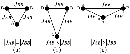
Figure 2: (a) A fully-frustrated triangular lattice. (b) A distorted triangular lattice realized in the room-temperature KNiCl₃-family of Fig. 1 (b). Since the interaction between A and B is weaker than that between B and B, two B-spins form antiferromagnetic state, while an A-spin takes an up or down state randomly. This is the PD configuration. (c) Another distorted lattice realized in Fig. 1 (c). Since $|J_{AB}|>|J_{BB}|$, A- and B- spins form antiferromagnetic state. This is the ferrimagnetic configuration.

3 Method

We observe the following two physical quantities. One is the sublattice order parameter:

$$m_{\eta}^{\mathrm{L}} = \frac{1}{N_{\mathrm{sub}}}\sum_{i}\sum_{j\in\eta}\sigma_{ij}$$ (8)

$$m_{\eta}^{\mathrm{S}} = \frac{1}{N_{\mathrm{sub}}}\sum_{i}\sum_{j\in\eta}S_{ij},$$ (9)

where $\eta=\alpha,\beta,\gamma$ denotes one of three sublattices in the triangular lattice, and $N_{\mathrm{sub}}$ denotes a number of sites in one sublattice. $m_{\eta}^{\mathrm{L}}$ is sublattice polarization and $m_{\eta}^{\mathrm{S}}$ is sublattice magnetization. The other physical quantity is the $1/3$ structure factor defined using sublattice polarization/magnetization:

$$f_{1/3}^{\mathrm{L}} = \frac{1}{2}\left\langle\sum_{\eta}(m_{\eta}^{\mathrm{L}})^{2}-(m_{\eta}^{\mathrm{L}}m_{\eta^{\prime}}^{\mathrm{L}}+m_{\eta}^{\mathrm{L}}m_{\eta^{\prime\prime}}^{\mathrm{L}})/2\right\rangle^{1/2}$$ (10)

$$f_{1/3}^{\mathrm{S}} = \frac{1}{2}\left\langle\sum_{\eta}(m_{\eta}^{\mathrm{S}})^{2}-(m_{\eta}^{\mathrm{S}}m_{\eta^{\prime}}^{\mathrm{S}}+m_{\eta}^{\mathrm{S}}m_{\eta^{\prime\prime}}^{\mathrm{S}})/2\right\rangle^{1/2}$$

$$(\eta\neq\eta^{\prime}\neq\eta^{\prime\prime}).$$

These structure factors take definite values when the Ferri or the PD state is realized and vanish when the symmetric/paramagnetic state is realized at high temperatures. $f^{\mathrm{L}}_{1/3}$ detects a phase boundary between an symmetric lattice phase and an deformed lattice phase. $f^{\mathrm{S}}_{1/3}$ detects a phase boundary between a magnetic order phase and the paramagnetic phase.

The sublattice order parameters distinguish the Ferri state and the PD state in an deformed/ordered phase. If one of three sublattice order parameters vanishes and the other two remain finite, the PD state is considered to be realized. If three sublattice order parameters take finite values, the Ferri state is considered to be realized.

We adopt the nonequilibrium relaxation method [16, 17, 18] to detect phase boundaries. This method utilizes a relaxation function of a physical quantity in Monte Carlo simulations. First, an ordered state is prepared as an initial state of simulations. We perform a simulation and obtain a relaxation function of a physical quantity. Another simulation is performed changing the random number sequence and another relaxation function is obtained. We take an average of relaxation functions over these independent Monte Carlo simulations. This sample average is free from a systematic error due to averaging correlated data. If the relaxation function of an order parameter exhibits an exponential decay, the system is judged to be in the paramagnetic phase. If it exhibits a converging behavior to a finite value, the system is in the ordered phase. The relaxation function exhibits an algebraic (power-law) decay at the critical point. The method has been verified to be particularly efficient in slow-dynamic systems with frustration and randomness.[19, 20, 21]

In the present simulation both spin and lattice variables at each lattice point are updated simultaneously using the heat-bath probability. We have checked that the Metropolis updating algorithm and the heat-bath updating algorithm yield the same relaxation behavior but with different correlation time. A simulation of the heat-bath is about four times faster as shown in Fig. 3.

Figure 3: A comparison between the Metropolis updating and the heat-bath updating. The NER functions of the structure factors behave in the same manner while the correlation time is about four times smaller in the heat-bath updating. An initial state is (lattice, spin)=(Ferri, PD).

The most important point in the NER method is to exclude out the finite-size effect from the raw relaxation function. The method is based upon taking the infinite-size limit first. If a relaxation function is affected by a finite-size effect, the relaxation behavior misleads us into thinking that the temperature is in the paramagnetic phase even though it is in the ordered phase. A lattice size of the present system is $L\times(L+1)\times 10L$ with $L$ ranging from $L=24$ to 120. We have checked the size dependence as shown in Fig. 4. The figure exhibits that the size effect appears quite early in the Monte Carlo step. A system with $L=120$ is confirmed to be free from the finite-size effect until one hundred steps in this figure. For every parameter point of $\kappa$ and temperature we have checked the size effect by comparing data of $L=120$ and $L=96$ and confirmed a time range that the data are free from the size effect. Results of $L=120$ are presented in this paper.

Figure 4: Size dependences of the structure factor of the spin. Data of sizes smaller than $L=96$ notably deviate from data of $L=120$. An initial state is (lattice, spin)=(Ferri, Ferri).

Initial conditions of the present simulations are mostly the ground-state configuration: the lattice structure is $P6_{3}cm$ and the magnetic structure is ferrimagnetic. This combination is referred to as (lattice, spin)=(Ferri, Ferri). We have also carried out simulations with initial configurations of (lattice, spin)=(Ferri, PD), (Ferri, Para), (PD, PD) and (Para, Para) in order to exclude out a possibility of initial state dependence in the final conclusion.

Computations are carried out by a PC cluster with 14 nodes consisting of Pentium-4 and Athlon-XP CPU. Total computation time is eighty days.

4 Results

4.1 The $1/3$ structure factor

The first issue is to make it clear whether the structural phase transition and the magnetic phase transition occur at the same temperature or not. The NER of the $1/3$ structure factor identifies the temperature that a lattice deformation or a magnetic order appears.

Figure 5: NER plots of the $1/3$ structure factors of the lattice and the spin at $\kappa=1.0$. The temperature is as denoted aside each plot. The structural transition and the magnetic transition occur at different temperatures.

Figure 5 shows NER plots of the structure factors at $\kappa=1.0$. We have started the simulation with an initial configuration of (lattice, spin)=(Ferri, Ferri). This combination is realized in the ground state. The NER of the structure factor of the lattice exhibits an exponential decay for $T\geq 11.25$. It exhibits a converging behavior for $T\leq 10.0$. The structural phase transition is considered to occur at $T_{\mathrm{c}}=10.625\pm 0.625$. The spin is still paramagnetic at this temperature. The NER of the structure factor of the spin shows that the magnetic phase transition occurs between $T=7.5$ and $T=9.0$ ($T_{\mathrm{c}}=8.25\pm 0.75$). Therefore, two transitions occur at different temperatures. Since the structural transition temperature is higher than that of the magnetic transition, the lattice system is considered to dominate the whole system at $\kappa=1.0$.

We have carried out the same analysis changing a value of $\kappa$ as listed in eq. (7) and found that the simultaneous transition may occur at $\kappa\simeq 1.6$ as shown in Fig. 6. Both structure factors decay exponentially for $T\geq 11.25$ and converge to finite values for $T\leq 11.00$. The transition temperature is estimated as $T_{\mathrm{c}}=11.125\pm 0.125$. For $\kappa=2.0$ and 2.5 it is found that the magnetic transition occurs at a higher temperature than a structural transition temperature. (Figures are not shown in this paper. Detailed data have been reported in the master thesis of one of the authors (T. S.). [22]) Therefore, there must be a point near $\kappa=1.6$ and $T=11.125$ that the simultaneous transition occurs.

Figure 6: NER plots of the $1/3$ structure factors of the lattice and the spin at $\kappa=1.6$. The simultaneous transition occurs near $T=11.125$.

4.2 Sublattice polarization/magnetization

We have observed the NER of sublattice polarization and sublattice magnetization in order to identify a lattice structure and a magnetic structure at low temperatures. It should be noticed that a sublattice may change its role of taking magnetization of $\uparrow$, $\downarrow$ or 0 depending on samples of independent Monte Carlo simulations. For example, when we start a simulation from the paramagnetic state at a temperature that the PD state is realized, one sublattice may take any three states of $\uparrow$, $\downarrow$ and 0 in each Monte Carlo simulation. Therefore, a simple average of sublattice magnetization over the independent Monte Carlo simulations yields an average of magnetization over sublattices: magnetization is obtained. In order to distinguish the above ambiguity, we collect data of sublattice magnetization depending on their value. Sublattice magnetization whose value is the smallest among three is stored in $m_{\mathrm{min}}^{\mathrm{S}}$. For example, a spin-down sublattice ($\downarrow$) in the PD state contributes to this variable. That of the largest value is stored in $m_{\mathrm{max}}^{\mathrm{S}}$ ($\uparrow$ in PD), and the rest is stored in $m_{\mathrm{mid}}^{\mathrm{S}}$ (0 in PD).

Figure 7: NER plots of squared sublattice polarization (lattice) and squared sublattice magnetization (spin) at $\kappa=1.0$ and $T=6.25$. The lattice Ferri state and the magnetic PD state are realized.

Figure 7 shows the NER of squared sublattice polarization/magnetization at $\kappa=1.0$ and $T=6.25$. The initial state is (lattice, spin)=(Ferri, Ferri). Three sublattice polarization converge to finite values. Here, $m_{\mathrm{min}}^{\mathrm{L}}$ corresponds to $\downarrow$-state and its squared value is largest among three. $m_{\mathrm{mid}}^{\mathrm{L}}$ and $m_{\mathrm{max}}^{\mathrm{L}}$ correspond to $\uparrow$-state and converge to the same value. A realized state is considered to be the lattice Ferri ($P6_{3}cm$). The NER of squared sublattice magnetization suggests that the magnetic structure is the PD state. $m_{\mathrm{min}}^{\mathrm{S}}$ and $m_{\mathrm{max}}^{\mathrm{S}}$ respectively correspond to the $\downarrow$-state and the $\uparrow$-state and converge to a finite value. $m_{\mathrm{mid}}^{\mathrm{S}}$ vanishes exponentially. Therefore, it is concluded that (lattice, spin)=(Ferri, PD) state is realized at $\kappa=1.0$ and $T=6.25$. We have verified this result by starting simulations with (Ferri, PD) state, (PD, PD) state and (Ferri, Para) state. Every relaxation plot has drawn out the same conclusion.[22]

Figure 8: The NER of sublattice polarization/magnetization at $\kappa=1.6$. The realized state is (lattice, spin)=(Para, Para) at $T=11.25$, while it is (lattice, spin)=(Ferri, Ferri) at $T=11.00$.

Figure 8 shows the NER of polarization/magnetization at $\kappa=1.6$ just above and below the simultaneous transition temperature. All the relaxation functions decay exponentially at $T=11.25$. This evidence suggests that both lattice and spin take symmetric/paramagnetic configurations at this temperature. Contrary, the relaxation functions converge to finite values at $T=11.00$. The (lattice, spin)=(Ferri, Ferri) state is considered to be realized. This is the ground state configuration. A direct transition from the high temperature phase to the ground-state phase has occurred. Intermediate phases vanish at this point.

5 Discussion

Putting all the NER results together we obtain a $T$-$\kappa$ phase diagram of the present model as shown in Fig. 9. When there is no spin degree of freedom at $\kappa=0$, successive structural phase transitions occur from the symmetric phase ($P6_{c}/mmc$) to the lattice PD phase ($P\bar{3}c1$) and then to the lattice Ferri phase ($P6_{3}cm$). Contrary, when there is no lattice degree of freedom at $\kappa=\infty$, we have also confirmed that successive magnetic transitions occur from the paramagnetic phase to the PD phase and then to the ferrimagnetic phase.

In case where both lattice and spin exist, a structural transition and a magnetic transition occur. If an energy scale of the lattice is larger than that of the spin ($\kappa\leq 1.3$), the structural transition occurs at a higher temperature than magnetic transition temperatures. At this transition temperature a lattice changes its structure directly from the symmetric one to the ground-state one. The intermediate phase does not appear. The successive magnetic transitions occur at lower temperatures. This interesting phenomenon can be explained by the following scenario. A key concept is relaxation of frustration.

A system with a larger energy scale becomes a master and the other one becomes a slave. When the structural transition occurs at a higher temperature, the lattice is a master and the spin is a slave. The spin as a slave serves a master relaxing frustration of the lattice by taking the PD configuration. As explained in Fig. 2, the spin favors the PD configuration when the lattice takes the Ferri structure, and vice versa. Since the temperature is still high, the PD spin configuration cannot be a long-range order. However, the short-range order is sufficient to relax frustration. The lattice can take the ground-state configuration without experiencing the intermediate PD phase.

A phase boundary of the structural transition does not depend on $\kappa$ when $\kappa\leq 1.3$, and smoothly interpolate to the phase boundary between Para and PD at $\kappa=0$. It is speculated that the structural PD phase suddenly vanishes by an introduction of an infinitesimal spin degree of freedom. When the temperature is lowered, the successive magnetic transitions occur. There is no slave relaxing frustration of the spin variable. Therefore, the intermediate phase appears.

Roles of the lattice and the spin are completely exchanged when an energy scale of the spin part exceeds that of the lattice part for $\kappa>1.6$. The spin becomes a master and the lattice becomes a slave. The magnetic transition occurs at a higher temperature and the ground-state configuration (ferrimagnetic state) is realized by an assistance of the lattice system. The successive structural transitions occur at lower temperatures.

The simultaneous magneto-dielectric transition occurs when two energy scales coincide. Either system relaxes frustration of the other system cooperatively. Both realize the ground-state configuration at the same temperature. Intermediate phases of both systems vanish. The simultaneous transition temperature corresponds to the real temperature as

$$(T_{\mathrm{c}}/|J_{1}^{\mathrm{L}}|)\times J_{1}^{\mathrm{S}}/\kappa=11.125\times 2.5/1.6\simeq 17\mathrm{K}.$$ (12)

It is almost half the experimental result of 37K. This underestimate is due to adopting the large reductions of exchange integrals: $\Delta J_{(c,1,2)}^{\mathrm{S}}=0.2J_{(c,1,2)}^{\mathrm{S}}$. The exchange integrals can be reduced to 60% of the original value. We made the reduction large in order to observe the spin-lattice cooperative phenomenon easily. However, it decreases an energy scale of the spin part, and consequently decreases the magnetic transition temperature. There is also an ambiguity in an experimental estimate of $J_{1}^{\mathrm{S}}$. Therefore, we consider that our estimate of the transition temperature is not inconsistent with the experimental result.

This scenario possibly explains the simultaneous transition in RbCoBr₃. It is also speculated that there is no further magnetic transition at lower temperatures. The ground-state magnetic state (possibly the ferrimagnetic state) is considered to be realized below the simultaneous transition temperature. Recently, it is reported that a single-crystal neutron diffraction experiment has revealed that all three sublattice magnetization are ordered at 37K.[23] This experimental evidence supports our speculation of an appearance of the ferrimagnetic state at the simultaneous transition point.

Figure 9: A phase diagram of the present model. Symbols discriminate phases as denoted in brackets.

In this paper we have introduced a model Hamiltonian which explains magneto-dielectric phase transitions in ABX₃-type compounds. It is supposed that any deformation of a lattice decreases the magnetic exchange interaction. The model is made as simple as possible just to understand the phenomenon qualitatively. Choices of the system parameters are not realistic. Therefore, there remains much to improve in order to compare theoretical results with experimental results quantitatively.

An essential point of this phenomenon is relaxation of frustration by introducing two systems: lattice and spin. Frustration finds a way to be relaxed by utilizing the other system. If it is relaxed, the intermediate phase like the PD phase vanishes. It can be considered that the intermediate phase is a product of frustration that has nowhere to go.

The authors would like to thank Professor Tetsuya Kato for guiding their interests to the present phenomenon and for fruitful discussions. The author T.N. also thank Yoichi Nishiwaki for fruitful discussions. The use of random number generator RNDTIK programmed by Professor Nobuyasu Ito and Professor Yasumasa Kanada is gratefully acknowledged.

References

- [1] N. Achiwa: J. Phys. Soc. Jpn. 27 (1969) 561.
- [2] M. Mekata: J. Phys. Soc. Jpn. 42 (1977) 76.
- [3] K. Adachi, N. Achiwa and M. Mekata: J. Phys. Soc. Jpn. 49 (1980) 545.
- [4] H. Shiba: Prog. Theor. Phys. 64 (1980) 466.
- [5] K. Adachi, K. Takeda, F. Matsubara, M. Mekata and T. Haseda: J. Phys. Soc. Jpn. 52 (1983) 2202.
- [6] H. Takayama, K. Matsumoto, H. Kawahara and K. Wada: J. Phys. Soc. Jpn. 52 (1983) 2888.
- [7] F. Matsubara and S. Inawashiro: J. Phys. Soc. Jpn. 53 (1984) 4373.
- [8] J. Wang, D. P. Belanger and B. D. Gaulin: Phys. Rev. B 49 (1994) 12299.
- [9] T. Kurata and H. Kawamura: J. Phys. Soc. Jpn. 64 (1995) 232.
- [10] O. Koseki and F. Matsubara: J. Phys. Soc. Jpn. 69 (2000) 1202.
- [11] T. Kato, K. Machida, T. Ishii, K. Iio and T. Mitsui: Phys. Rev. B 50 (1994) 13039.
- [12] K. Morishita, N. Nakano, T. Kato, K. Iio and T. Mitsui: Ferroelectrics 217 (1998) 207.
- [13] K. Morishita, T. Kato, K. Iio, T. Mitsui, M. Nasui, T. Tojo and T. Atake: Ferroelectrics 238 (2000) 105.
- [14] T. Kato: private communication.
- [15] K. Morishita, K. Iio, T. Mitsui and T. Kato: J. Magn. Magn. Mater. 226-230 (2001) 579.
- [16] D. Stauffer: Physica A 186 (1992) 197.
- [17] N. Ito: Physica A 196 (1993) 591.
- [18] N. Ito and Y. Ozeki: Int. J. Mod. Phys. 10 (1999) 1495.
- [19] T. Shirahata and T. Nakamura: Phys. Rev. B 65 (2002) 024402.
- [20] T. Nakamura and S. Endoh: J. Phys. Soc. Jpn. 71 (2002) 2113.
- [21] T. Nakamura: J. Phys. Soc. Jpn. 72 (2003) 789.
- [22] T. Shirahata: Mr. Thesis, Department of Applied Physics, Tohoku University, Aoba, Sendai, 2002 [in Japanese].
- [23] Y. Nishiwaki, T. Kato, Y. Oohara and K. Iio: in preparation.