On The Possibility of Quasi Small-World Nanomaterials

Abstract

The possibility of materials that are governed by a fixed point related to small world networks is discussed. In particular, large-scale Monte Carlo simulations are performed on Ising ferromagnetic models on two different small-world networks generated from a one-dimensional spin chain. One has the small-world bond strengths independent of the length, and exhibits a finite-temperature phase transition. The other has small-world bonds built from atoms, and although there is no finite-temperature phase transition the system shows a slow power-law change of the effective critical temperature of a finite system as a function of the system size. An outline of a possible synthesis route for quasi small-world nanomaterials is presented.

I Introduction

Many materials have novel physical properties that are attributed to the quasi-low-dimensional nature of their structure, as can be seen in recent research in a number of areas. Examples of quasi-one-dimensional materials include conductors and superconductors JERO87 . Two-dimensional thin films lead to novel effects, including the quantum Hall effect PELE03 and low-dimensional magnetism SVIS03 . The change from one effective dimension to another may lead to interesting physical effects. For example, it may be responsible for the onset of high-temperature superconductivity MENZ02 . This type of dimensional crossover can lead to effective non-integer dimensional fixed points NOVO93 . However, quasi-low-dimensional materials have constraints due to their low-dimensional behavior. These include the absence of a phase transition both in one-dimensional systems and in some two-dimensional systems where two is below the lower critical dimension.

Recently there has been a great deal of interest in networks that are not regular lattices, such as small-world networks BARA02 . The study of these networks has been motivated mainly by social organizations (such as six degrees of separation) and connectivities of computers (such as the scale-free world-wide-web network) BARA02 . Such connectivities have also been used, for example, in non-trivial parallelization of short-ranged discrete event simulations KORN99 ; KORN00 ; KORN02 ; KOLA03 ; KORN03 . Simulations of models such as Ising spin models on these networks have been studied, but no attempt has been made to ask whether these theoretical models could actually be designed and built via various synthesis routes. This question is addressed in this manuscript. There is a difference between the models studied to date and the question of whether or not materials can be made that are governed by small-world fixed-points. The difference is that materials must be constructed from atoms and must be embedded in three-dimensional space.

II Model and Methods

The models studied here are Ising models with $N_{0}$ spins on a linear chain, with a nearest-neighbor ferromagnetic interaction constant $J_{1}$.

In the first model, model 1, if there is a small-world connection between spins $i$ and $j$ and $i\geq j+1$ a ferromagnetic interaction of strength $J_{2}(i,j)$ is added. The Hamiltonian is

$${\cal H}=-J_{1}\sum_{i}\sigma_{i}\sigma_{i+1}-\sum_{\rm SW}J_{2}(i,j)\sigma_{i}\sigma_{j}$$ (1)

where periodic boundary conditions are used (spin $N_{0}+1$ equals spin 1) and the Ising spins $\sigma=\pm 1$. Terms in the second sum are only present if there exists a small world connection between spins $i$ and $j$. We construct a (random) small-world network algorithmically by: i) start with spin 1, and randomly connect it to any of the other $N_{0}-1$ spins; ii) if spin 2 is not connected to spin 1, then randomly connect it to one of the $N_{0}-2$ spins that are not already connected; iii) continue for all $N_{0}$ spins. Note that here $N_{0}$ must be even. This algorithm gives each spin $i$ three connections, two of strength $J_{1}$ to spins $i-1$ and $i+1$ and one of strength $J_{2}$ to the small-world connection between spin $i$ and $j$. This type of small-world connection has been used in the past to obtain perfectly scalable parallel discrete-event simulations KORN03 . A study of the Ising model on a similar small world network with $J_{2}(i,j)=Jr^{-\alpha}_{ij}$ (i.e. having a power-law dependence on distance) has recently been performed JEON03 . There they conclude that any non-zero value for $\alpha$ destroys the finite-temperature phase transition in the thermodynamic limit. This result differs from the case with $J_{2}(i,j)=J_{2}$ (independent of length), where a finite-temperature phase transition has been observed GITT00 ; BARR00 ; PEKA01 ; HONG02 ; KIM01 . Our first model has all small-world bonds of strength $J_{2}$, independent of length.

In our second model, model 2, we construct the small-world connections from Ising spins. In particular, for each small-world bond constructed as in our first model between spins $i$ and $j$, we add $r_{ij}+1$ Ising spins and couple each of them together with interactions of strength $J_{2}$. These additional Ising chains are coupled to the original Ising spins $i$ and $j$ with interaction strength $J_{2}$. Thus, the small-world connections have been constructed using the same lattice constant as the original lattice (but different nearest-neighbor interactions).

We have performed a standard importance-sampling Monte Carlo simulation LAND00 . We measured the magnetization $m=\sum_{i}\sigma_{i}/N_{\rm tot}$, order parameter, susceptibility $\chi$, internal energy, specific heat, and the Binder 4^th order cumulant for the order parameter $U=1-\frac{\left\langle m^{4}\right\rangle}{3\left\langle m^{2}\right\rangle^{2}}$. The code was run using trivial parallelization on a cluster, using up to 128 processing elements. The parallel random number generator SPRNG 1.0 SPRNG was used. The spins to be updated were chosen randomly, a Glauber spin-flip probability was used. For each temperature $T$, $10^{5}$ Monte Carlo steps per spin (MCSS) were used for thermalization and averages were taken over $10^{6}$ MCSS (with measurements taken every $10$ MCSS). The energy units were chosen such that $J_{1}/k_{\rm B}=1$, where $k_{\rm B}$ is Boltzmann’s constant. In this paper the choice $J_{2}=4J_{1}$ was made.

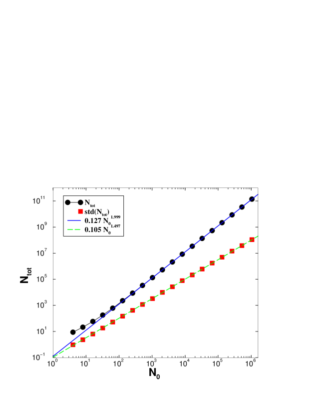
Figure 1: The total number of Ising spins $N_{\rm tot}$ as a function of the number of spins $N_{0}$ in the one-dimensional chain is shown. The solid line is a fit to the data for $N_{0}\geq 2^{10}$. Also shown is the standard deviation of $N_{\rm tot}$ from the mean (squares), and a fit to those data (dashed line).

III Data and Analysis

In our second model, one question is the average number of total Ising spins $N_{\rm tot}$ starting with a spin chain of length $N_{0}$. For a chain of length $L$ and lattice constant $a$, one has $L=N_{0}a$. Here we take the lattice spacing $a=1$, so $N_{0}=L$. It is shown in Fig. 1 that $N_{\rm tot}\propto N_{0}^{x}$ with exponent $x\approx 2$. A fit to data (averaged over $10^{3}$ different small-world bond connections) for $2^{10}\leq N_{0}\leq 2^{20}$ gives $N_{\rm tot}=0.127N_{0}^{1.999}$. A fit with the same range of $N_{0}$ for the standard deviation of the mean gives ${\rm std}(N_{\rm tot})=0.105N_{0}^{1.497}$.

The relationship $N_{\rm tot}\propto N_{0}^{2}$ can be understood easily in an approximate fashion, by ignoring correlations between the small-world interconnections. Although the number of spins scales as the square of the linear distance $N_{0}$, the fixed point governing the system is not expected to be the two-dimensional fixed point since the bond connectivity is different from that of a two-dimensional lattice. The average length of a connection is $N_{0}a/4$. This is because the lengths of the connections are chosen uniformly up to the maximum possible distance of a connection, which is $N_{0}a/2$ due to the periodic boundary conditions. There are $N_{0}/2$ such connections (the factor of 2 is to take into account double counting). Ignoring factors in the number of spins that are proportional to $N_{0}$ thus gives $N_{\rm tot}\approx\frac{1}{8}N_{0}^{2}$. As seen in the fit in Fig. 1, both the fitted exponent and prefactor are in excellent agreement with this argument for $N_{0}\geq 2^{7}$. An extension of this argument shows that if only a fraction $p_{\rm connect}$ of spins were connected, then the total number of spins should scale like $N_{\rm tot}\approx\frac{p_{\rm connect}}{8}N_{0}^{2}$ for large $N_{0}$. Simulations were performed with values of $N_{0}=8$ and for $N_{0}$ up to $N_{0}=16384$ for model 1 and $N_{0}=256$ for model 2.

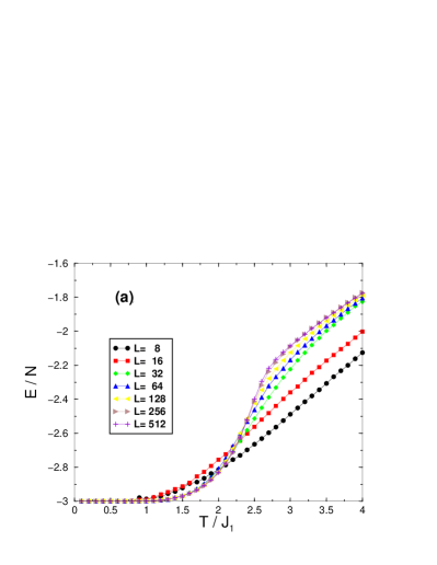
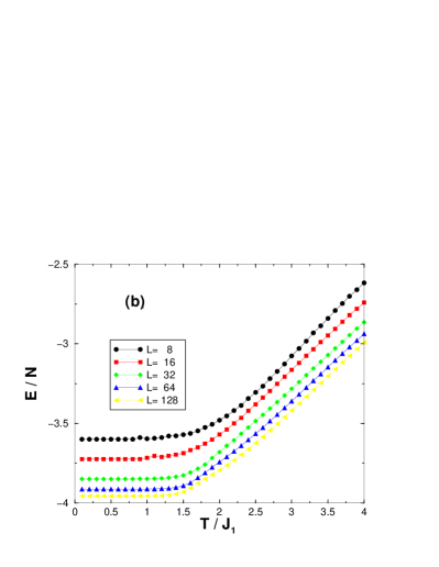
Figure 2: The internal energy per Ising spin for (a) model 1, and (b) model 2. These are parameterized by the chain length, $L=N_{0}a$, where $a$ is the lattice spacing and $N_{0}$ is the number of spins in the one-dimensional backbone.

Figure 2 shows the average internal energy per Ising spin, in units of $J_{1}$, as a function of temperature. The internal energy is the expectation value of the Hamiltonian, $E=\langle{\cal H}\rangle$. Model 1, Fig. 2(a), has the low-energy value for $E/N$ independent of $N$, since in the ground state (all spins the same direction) the energy is $E/N=(2J_{1}+J_{2})/2$ where the division by $2$ takes into account double counting. For model 1, $J_{1}=1$ and $J_{2}=4$, so $E/N=-3$ at low temperatures. Note that model 1 has a singularity developing with large $N$ near $T=2.5J_{1}$. Model 2, Fig. 2(b), looks different. Note that for model 2, this energy is divided by the total number of Ising spins, $N_{\rm tot}$. The ground-state energy per spin has the form $\frac{E}{N_{\rm tot}}=\frac{N_{0}\left(2J_{1}+J_{2}\right)+2J_{2}\left(N_{\rm tot}-N_{0}\right)}{2N_{\rm tot}}$, which at low temperatures approaches $-4$ since $N_{\rm tot}\gg N_{0}$ for large $N_{0}$.

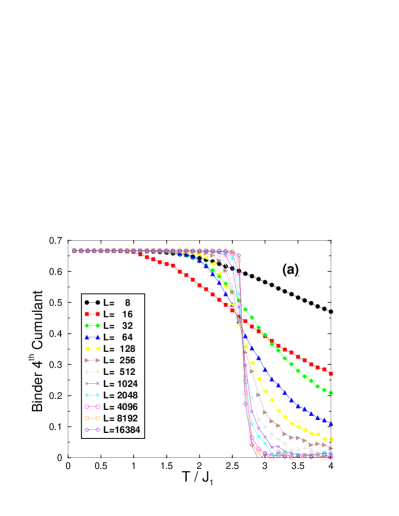
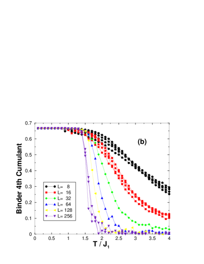
Figure 3: The Binder fourth-order cumulant for (a) model 1, and (b) model 2.

Figure 3 shows the Binder $4^{th}$-order cumulant for the magnetization as a function of the temperature for both models. The temperature where two of these curves for different $N_{0}$ cross is an estimate for the critical temperature. An alternative estimate can be obtained by choosing a value such as 0.5, and letting the estimate of the critical temperature be where the cumulant crosses the value of 0.5. (Ideally, one would like to use the value of the infinite-lattice cumulant, but this is often unknown unless the universality class of the model is known.) Model 1, Fig. 3(a), shows a very nice indication of a critical point near $T\approx 2.7J_{1}$. Model 2, Fig. 3(b), shows no such estimate of the critical point. Only by choosing the temperature where the cumulant crosses 0.5 can an estimate of the finite-size critical point (if it exists) be obtained. Note that for model 2 there are a number of different quenched small-world bond configurations for $N_{0}=8$, $16$, and $256$.

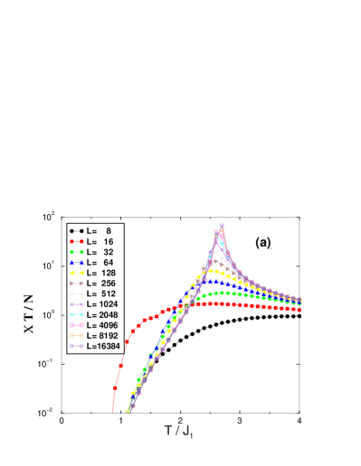
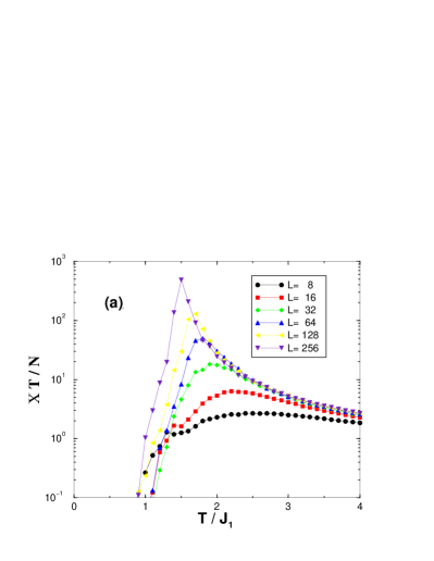
Figure 4: The susceptibility times temperature for (a) model 1, and (b) model 2.

Figure 4 shows the susceptibility $\chi$ per Ising spin times the temperature $T$. For model 1, Fig. 4(a), shows a sharpening maximum at $T\approx 2.7$. Figure 5, for model 1, shows the maximum value for $\chi T$ as a function of $N_{0}$. There are five different quenched small-world connections shown for each value of $N_{0}$. The slope of this log-log plot gives an estimate for the exponent ratio $\gamma/\nu$, with $\gamma$ the susceptibility exponent and $\nu$ the correlation length exponent. The value obtained for the slope is $0.73$ using all lattice sizes, and it is $0.65$ using only the sizes $256$ and $512$. Although simulations for larger $N_{0}$ may give lower slopes yet, we estimate that $\gamma/\nu=0.6\pm 0.1$.

The maxima of $\chi T/N_{\rm tot}$ for model 2, Fig. 4(b), decrease with temperature as $N_{0}$ increases. This indicates that there may be no finite-temperature phase transition in the thermodynamic limit. This conclusion is further supported in Fig. 6. There the location of both the crossing of the Binder cumulant and 0.5 and the maximum of $\chi T/N_{\rm tot}$ is shown. Both estimates for the ‘finite system-size’ critical point agree. They both also have a reasonable fit, based on $N_{0}\geq 32$, of $T_{\rm c}=AN_{0}^{x}$ with $x=-0.105$ and $A=2.74$.

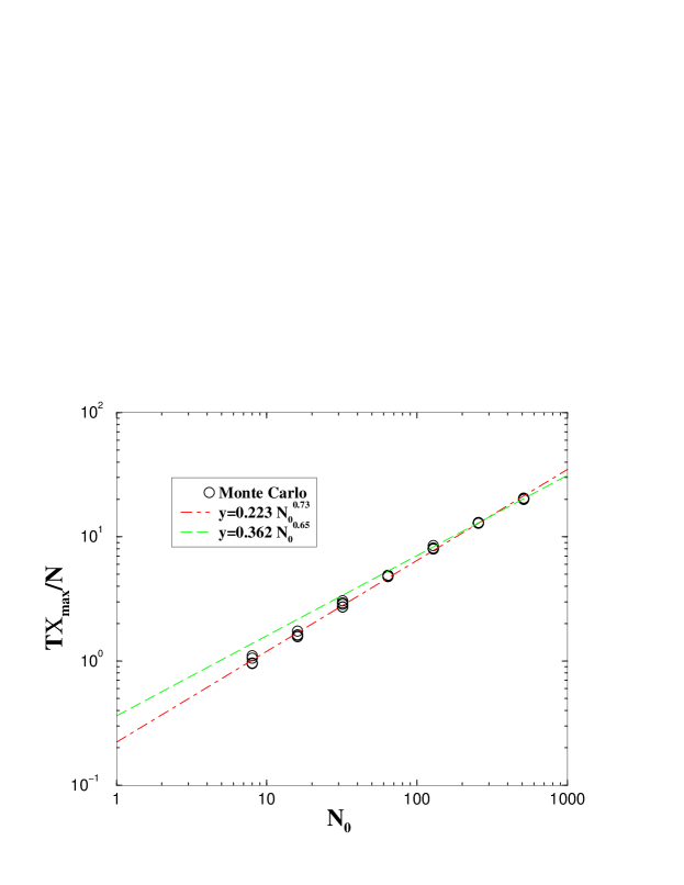
Figure 5: The maximum of the susceptibility times the temperature for model 1. The slope of this gives an estimate for the ratio of critical exponents $\gamma/\nu$.

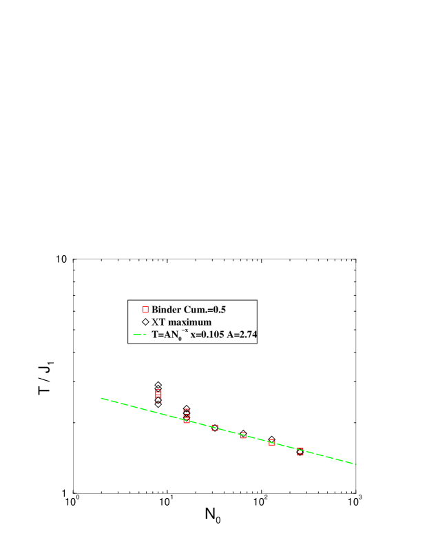
Figure 6: The summary for model 2 of the various indicators of critical behavior are shown as a function of the system size. Note that this fit (dashed line) suggests that a finite-temperature phase transition does not survive taking the thermodynamic limit.

IV Possibilities for Small World Materials

Model 2, with the small-world bonds built of atomic spins, exhibits no finite temperature phase transition in the thermodynamic limit. Consequently, the outlook for small-world materials is that they will not be easy to synthesize. Note that rigorously it has been shown that no finite temperature phase transition can occur in one dimension. Nevertheless, there are a large number of effective one-dimensional materials JERO87 . Small-world models with fixed connection sizes, such as model 1, exhibit a finite temperature critical point. Building these small-world connections from atomic spins as in model 2 provides the small-world bonds. However although the small-world fixed point is unstable at finite temperatures, the flow from this unstable fixed point seems to be extremely slow. Consequently, the outlook for quasi small-world materials is better than for quasi-one-dimensional materials.

Table I shows the effective $T_{\rm c,eff}$ for a given size of material for model 2. Also shown from ref. JEON03 are values of $T_{\rm c,eff}$ for small-world connections with strengths that behave as $J_{1}r_{ij}^{-\alpha}$, for different values of $\alpha$. All temperatures are in units of $J_{1}$. Due to the slow decrease in the critical point with the system size, Table I shows that even for large systems (of the size of meters) the system should exhibit an effective critical temperature that can still occur at a reasonably high temperature.

Material	$N_{\rm atom}$	$T_{\rm c}$	$T_{p}$	$T_{p}$	$T_{p}$
Size		added atoms	$\alpha=0.1$	$\alpha=0.2$	$\alpha=0.3$
base	$1$	$2.74$	$1.62$	$1.67$	$1.69$
$\mu$m	$5\times 10^{3}$	$1.12$	$1.48$	$1.31$	$1.69$
mm	$5\times 10^{6}$	$0.54$	$1.37$	$1.02$	$0.70$
m	$5\times 10^{9}$	$0.26$	$1.26$	$0.73$	$0.26$

Table 1: Extrapolated values for the finite-size effective critical temperature (for example $T_{p}$, the location of the maximum in $\chi T$) for various sizes corresponding to the given number of atoms in a one-dimensional chain material. See the text for the assumptions. The last three columns represent the data of ref. JEON03 , as explained in the text.

One synthesis route for small-world nanomaterials is described here. This is a theorist’s cartoon of the synthesis route, and consequently is not meant to be detailed. First, start by constructing a one-dimensional chain of atoms (or molecules), most likely embedded on the surface of a support material. Prepare a solution of linear molecules of all different lengths up to the maximum size of material to be synthesized. This could be accomplished by starting with linear molecules of the same length, and then having a chemical process that breaks the linear chains at random locations. Place a reactive agent at the ends of these linear segments, this agent should be reactive with the constructed one-dimensional chain of atoms on the surface of the material. Bring this constructed chain of atoms into contact with the solution of reactive linear molecules, forming the small-world connections. A further synthesis step can be performed to reduce the length of the linear molecules to the minimum possible distance. This could be accomplished by removing atomic segments. The material synthesized in this way should mimic closely the small-world connections of model 2.

There are several factors that may make quasi small-world nanomaterials easier to synthesis than the synthesis route outlined above. It has been shown that not all original atoms (ones that are not in the small-world connections) need to be connected with small-world bonds for the system to be controlled by the small-world fixed point KORN03 ; JEON03 . Rather, what is required is just a finite density of small-world bonds. Hence, the prefactor in front of the power law for the number of total atoms per original atom may be made arbitrarily small. It is also possible to consider starting with a two-dimensional thin film, and synthesizing small-world connections on the film in a fashion similar to the one-dimensional route outlined above. Some studies of crossover from two- and three-dimensional fixed points to small-world fixed points have been performed HERR02 ; HAST03 . However, it is anticipated that for any finite density of small-world connections the dominant fixed point should be the small-world fixed point. Furthermore, since these original one and two-dimensional systems are embedded in three dimensions, it is possible to make some of the longer-distance small-world connections very short-ranged by bending or folding the original lattice to minimize the total length of all small-world bond connections. Finally, just as in quasi-one-dimensional materials there is the possibility of allowing weak interactions in three dimensional crystals to stabilize the fixed point in different dimensions before the system exhibits a cross-over to the three-dimensional fixed point.

V Discussion and Conclusions

The ferromagnetic Ising model on two small-world networks has been studied. One model, related to models previously studied by others GITT00 ; BARR00 ; PEKA01 ; HONG02 ; KIM01 , has only fixed-strength interactions for the small-world connections. This model exhibits a finite-temperature second-order phase transition. We have determined from finite-size scaling of the maximum of the susceptibility the exponent ratio $\gamma/\nu=0.6(1)$ for the system sizes simulated. A study by other researchers with small-world connections that fall off as a power-law with actual distance shows no finite-temperature phase transition, but a logarithmic decrease with $N_{0}$ of an effective finite system size critical temperature $T_{\rm c,eff}$JEON03 .

The second Ising model studied here is more realistic for the possibilities of quasi small-world materials. The small-world connections have been constrained to be built from spins using the same lattice spacing. This models what would have to be accomplished in actual quasi small-world materials, since atoms are the fundamental building blocks. For this model, no finite-temperature phase transition was found to survive the thermodynamic limit. In particular, in terms of the number of linear spins $N_{0}$, an effective critical temperature $T_{\rm c,eff}$ was found to behave as $N_{0}^{x}$ with $x\approx-0.105$. Furthermore, on general grounds the total number of spins scales as $N_{\rm tot}\sim N_{0}^{2}$ for a one-dimensional system with $N_{0}$ spins.

From these studies a theoretical picture emerges about the difficulty in synthesizing quasi small-world materials. The number of atoms needed to connect small-world bonds may be large, and is expected to scale as a power law of the number of atoms in the none small-world system. However, it has been shown that not all none small-world atoms need to be connected with small-world bonds for the system to be controlled by the small-world fixed point KORN03 ; JEON03 . Consequently, the prefactor in front of the power law for the number of small-world atoms may be made arbitrarily small in principle. For strengths of small-world connections that decrease as a power law JEON03 , a logarithmic fall-off of the effective critical temperature with system size has been found. Using some order-of-magnitude assumptions and the different power law results from this work and ref. JEON03 , one finds that a reasonable value of $T_{\rm c,eff}$ is possible for systems in the size ranges of microns, millimeters, or even meters. For the model studied here, where the small-world connections were built from atomic spins, a small power-law fall-off of the effective critical temperature was found. Thus nanoscale and mesoscale materials should exhibit an effective critical behavior related to the small-world bonds. A possible synthesis route to materials effectively governed by small-world fixed points was outlined.

VI Acknowledgements

I acknowldge useful discussions with a number of people, particularly Torsten Clay, Seong-Gon Kim, Alice Kolakowska, Gyorgy Korniss, Chris Landee, Per Arne Rikvold, and Zoltan Toroczkai. Supported in part by NSF grants DMR-0120310 and DMR-0113049. Computer time from the Mississippi State University ERC and NERSC was critical to this study.

References

- (1) Low Dimensional Conductors and Superconductors, NATO ASI Series B, Phys. Vol. 155, editor D. Jerome and L.G. Caron (Plenum, New York, 1987).
- (2) E. Peled, D. Shahar, Y. Chen, D.L. Sivco, and A.Y. Cho, Phys. Rev. Lett. 90, 246802 (2003).
- (3) L.E. Svistov, A.I. Smirnov, L.A. Prozorova, A.O. Petrenko, L.N. Dernianets, and A.Ya. Shapiro, Phys. Rev. B 67, 094434 (2003).
- (4) A. Menzel, R. Beer, and E. Bertel, Phys. Rev. Lett. 89, 076803 (2002).
- (5) M.A. Novotny, Phys. Rev. Lett. 70, 109 (1993).
- (6) R. Albert and A.-L. Barabási, Rev. Mod. Phys. 74, 47 (2002).
- (7) G. Korniss, M.A. Novotny, H. Guclu, Z. Toroczkai, and P.A. Rikvold, Science 299, 677 (2003).
- (8) G. Korniss, Z. Toroczkai, M.A. Novotny, and P.A. Rikvold, Phys. Rev. Lett. 84, 1351 (2000).
- (9) A. Kolakowska, M.A. Novotny, and G. Korniss, Phys. Rev. E 67, 046703 (2003).
- (10) G. Korniss, M.A. Novotny, P.A. Rikvold, H. Guclu, and Z. Toroczkai, Materials Research Society Symposium Proceedings Series Vol. 700, p. 297 (2002).
- (11) G. Korniss, M.A. Novotny, and P.A. Rikvold, J. Comp. Phys. 153, 488 (1999).
- (12) D. Jeong, H. Hon, B.J. Kim, and M.Y. Kim, preprint arXiv:cond-mat/0306017.
- (13) M. Gitterman, J. Phys. A: Math. Gen. 33, 8373 (2000).
- (14) A. Barrat and M. Weigt, Eur. Phys. J. B 13, 547 (2000).
- (15) A. Pekalski, Phys. Rev. E 64, 057104 (2001).
- (16) H. Hong, B.J. Kim, and M.Y. Choi, Phys. Rev. E 66, 018101 (2002).
- (17) B.J. Kim, H. Hong, P. Holme, G.S. Jeon, P. Minnhagen, and M.Y. Choi, Phys. Rev. E 64, 056135 (2001).
- (18) D.P. Landau and K. Binder, A Guide to Monte Carlo Simulations in Statistical Physics (Cambridge University Press, Cambridge, UK, 2000).
- (19) See http://sprng.cs.fsu.edu
- (20) C.P. Herrero, Phys. Rev. E 65, 066110 (2002).
- (21) M.B. Hastings, preprint arXiv:cond-mat/0304530.