Generic properties of a quasi-one dimensional classical Wigner crystal

Abstract

We studied the structural, dynamical properties and melting of a quasi-one-dimensional system of charged particles, interacting through a screened Coulomb potential. The ground state energy was calculated and, depending on the density and the screening length, the system crystallizes in a number of chains. As a function of the density (or the confining potential), the ground state configurations and the structural transitions between them were analyzed both by analytical and Monte Carlo calculations. The system exhibits a rich phase diagram at zero temperature with continuous and discontinuous structural transitions. We calculated the normal modes of the Wigner crystal and the magneto-phonons when an external constant magnetic field $B$ is applied. At finite temperature the melting of the system was studied via Monte Carlo simulations using the $modified$ $Lindemann$ $criterion$ (MLC). The melting temperature as a function of the density was obtained for different screening parameters. Reentrant melting as a function of the density was found as well as evidence of directional dependent melting. The single chain regime exhibits anomalous melting temperatures according to the MLC and as a check we study the pair correlation function at different densities and different temperatures, which allowed us to formulate a different criterion. Possible connection with recent theoretical and experimental results are discussed and experiments are proposed.

I INTRODUCTION

Recently there has been a great deal of interest in mesoscopic systems consisting of interacting particles in low dimensions or confined geometries. A class of quantum anisotropic systems exhibiting “stripe” behavior appears in the quantum Hall effect qhestripes , in oxide manganites and high-T_c superconductors hightc where electronic strong correlations are responsible for the formation of these inhomogeneous phases. Another class of confined quasi one-dimensional (Q1D) geometries appears in many diverse fields of research and some typical and important examples from the experimental point of view are : electrons on liquid Helium glasson ; kovdrya , microfluidic devices whitesides , colloidal suspensions zahn and confined dusty plasma chu .

A major phenomenon which is expected to occur in charged particles interacting via a Coulomb or screened Coulomb potential is Wigner crystallization (WC) wigner at low enough temperatures and densities when the potential energy overwhelms the kinetic energy. Indeed, evidence of such a type of transition was found very recently glasson in experiments on electrons on the surface of liquid Helium where the electrons were confined by metallic gates and exhibited dynamical ordering in the form of filaments. This particular experiment posed many interesting questions regarding the nature of the transition to WC, its density dependence and the melting. Furthermore, the considered system has been proposed as a possible step towards the realization of a quantum computer with electrons floating on liquid Helium platzman .

In this paper, as a first step towards the understanding of the behavior of these systems, we start with a two-dimensional system consisting of an infinite number of charged particles and we impose a parabolic confining potential in one direction. The particles interact with a Yukawa-type potential where the screening length is an external parameter. Physically, it can be adjusted e.g. by the gate voltage that confines the electrons. The combination of the interaction among particles and the external potential leads to a rich structural phase diagram as a function of the screening length $\lambda$ and the density $n$ of the system. The structural units (at temperature $T=0K$) are parallel chains of particles the number of which depend on the values of $\lambda$ and $n$. The transition from one configuration to the other can be obtained via a first or a second order transition.

Before proceeding further, we should comment on the possibility of two-dimensional crystalline order. According to the Mermin-Wagner theorem Mermin there is no true long-range crystalline order in two dimensions. However this theorem is only strictly valid when the potential falls off faster than $1/r$ and in the thermodynamic limit. When the same arguments of the theorem are applied to a large but finite system, no inconsistencies arise from the assumption of crystalline order. Thus any system that can be studied in laboratory or in computer simulations can exhibit crystalline order Gann . On the other hand short-range order is expected to form even in the thermodynamic limit.

In a related work dubin which discussed the temperature equilibration of a one-dimensional Coulomb chain, two different equilibration temperatures were assigned ($T_{\perp}$ and $T_{||}$), reflecting the different behavior of the modes due to the strong confinement.

The WC in strictly one dimension and in the quantum regime was first studied by Schultz schultz . He found that for arbitrarily weak Coulomb interaction the density correlations at wave vector $4k_{F}$ decay extremely slowly (the most slowly decay term is $\propto\exp{(-c\sqrt{\ln{x}})}$ .

Other remarkable work on the quantum transport and pinning in the presence of weak disorder, where it was shown that quantum fluctuations soften the pinning barrier and charge transfer occurs due to thermally assisted tunneling, is described in glazman .

In addition to the structural properties, it is instructive to study the normal modes of these kind of anisotropic systems. There are optical and acoustical branches and their number is equal to the number of chains. The acoustical modes correspond to motion along the unconfined direction and the optical ones to motion along the confined direction. There is softening of an optical phonon at those values of the density for which we have a continuous structural transition. We also study the collective excitations in the presence of a constant magnetic field perpendicular to the plane of the system. These modes (magnetophonons), can be directly detected experimentally magn1 ; magn2 .

Another important aspect of the problem is the melting as the temperature is raised. The mechanisms of melting is of great scientific and technological importance. In infinite two-dimensional (2D) systems theory kthny , based on unbinding of defects, predicts a two-stage melting where the two stages are continuous. Recent theoretical studies of melting of colloidal crystals in the presence of a one-dimensional periodic potential radzihovsky revealed a number of novel phases and the possibility of reentrant melting. These results depend on the commensurability ratio $p=a/d_{ext}$ where $a$ is the spacing between the Bragg planes of the 2D system and $d_{ext}$ the period of the external periodic potential. This kind of system was realized experimentally wei in 2D colloids in the presence of two interfering laser beams. The present work is complementary to the work of Frey, Nelson and Radzihovsky radzihovsky in the sense that a single confining potential is considered here, which is not repeated in space. Therefore it can be viewed as a study of a focused portion of the infinite 2D system, where we pay attention to only one potential trough neglecting the interaction with the rest. With respect to the melting, we found the following remarkable results:(i) a phase diagram which exhibits reentrant melting behavior as a function of the density where the different configurations are explored, (ii) a regime of frustration exists close to the structural transitions, and (iii) there is evidence that the system first melts in the unconfined direction and subsequently in the direction where it is confined exhibiting a regime similar to the locked floating solid regime found in Ref. radzihovsky .

The paper is organized as follows. In Sec. II, we present the model and the methods used. In Sec. III we study the zero temperature phase diagram and properties of the structural transitions. Sec. IV is devoted to the study of the normal modes of the system and in the presence of, or without, an external magnetic field $B$. In Sec. V we study the melting and analyze furthermore in some details the problem of the single chain melting.

Finally we discuss the connections with recent experimental results and suggest experiments where this behavior can be observed in Sec. VI.

II MODEL AND METHODS

The system is modelled by an infinite number of classical charged particles with identical charge $q$, moving in a plane with coordinates $\vec{r}=(x,y)$. The particles interact through a Yukawa potential and an additional parabolic potential confines the particle motion in the $y$ direction. The Hamiltonian of the system is given by :

$$H=\frac{q^{2}}{\epsilon}\sum_{i\neq j}\frac{exp(-|\vec{r_{i}}-\vec{r_{j}}|/\lambda)}{|\vec{r_{i}}-\vec{r_{j}}|}+\sum_{i}\frac{1}{2}m{\omega_{0}}^{2}{y_{i}}^{2}$$ (1)

where $m$ is the mass of each particle, $\epsilon$ is the dielectric constant of the medium particles are moving in, $\omega_{0}$ measures the strength of the confining potential. The Hamiltonian can be rewritten in a dimensionless form, introducing the quantities $r_{0}=(2q/m\varepsilon\omega_{0}^{2})^{1/3}$ as unit of length and $E_{0}=(m\omega_{0}^{2}q^{4}/2\varepsilon^{2})^{1/3}$ as unit of energy. Then it takes the form

$$H^{\prime}=\sum_{i\neq j}\frac{exp(-\kappa|\vec{r^{\prime}_{i}}-\vec{r^{\prime}_{j}}|)}{|\vec{r^{\prime}_{i}}-\vec{r^{\prime}_{j}}|}+\sum_{i}{y^{\prime}_{i}}^{2}$$ (2)

where $H^{\prime}=H/E_{0}$, $\kappa=r_{0}/\lambda$ and $\overrightarrow{r}^{\prime}=\overrightarrow{r}/r_{0}$. This transformation is particularly interesting because now the Hamiltonian no longer depends on the specifics of the system and becomes only a function of the density and the dimensionless inverse screening length. The quantities introduced allow us to define a dimensionless temperature $T^{\prime}=T/T_{0}$ with $T_{0}=(m\omega_{0}^{2}q^{4}/2\varepsilon^{2})^{1/3}k_{B.}^{-1}$.

For the calculations of the ground state energy we used a combination of analytical calculations and Monte Carlo simulations with the standard Metropolis algorithm. This recursive algorithm consists in displacing randomly one particle and accepting the new configuration if its energy is lower than the previous one; if the new configuration has a larger energy the displacements are accepted with probability $\delta<\exp(-\Delta E/T)$, where $\delta$ is a random number between $0$ and $1$ and $\Delta E$ is the increment in the energy. We have allowed the system to approach its equilibrium state at some temperature $T$, after executing $10^{5}\div 10^{6}$ Monte Carlo steps. We have used the technique of simulated annealing to reach the $T=0$ equilibrium configuration: first the system has been heated up and then cooled down to a very low temperature. In the simulations typically 300 particles were used and in order to simulate an infinitely long system periodical boundary conditions (Born-Von Karman) were introduced.

III Ground state configurations

III.1 Phase Diagram

The charged particles crystallize in a certain number of chains. Each chain has the same density resulting in a total one-dimensional density $\widetilde{n}_{e}$. It is then possible to calculate the energy per particle for each configuration and to check the favored one as a function of the parameters of the system. If $a$ is the separation between two adjacent particles in the same chain, we can define the dimensionless linear density $\widetilde{n}_{e}=lr_{0}/a$, where $l$ is the number of chains.

In the case of multiple chains, in order to have a better packing (or in other words to minimize the interaction energy by maximizing the separation among particles in different chains), the chains are staggered with respect to each other by $a/2$ in the $x$ direction. In an infinite lattice this will lead to the hexagonal WC bonsall . We calculated the energy per particle as a function of the density for the first six possible configurations of the system.

If the particles crystallize in a single chain, the minimum energy is obtained when the particles are placed on the $y$ axis, where the confining potential is zero. In this case the linear density is $\widetilde{n}_{e}=r_{0}/a$ and the $x$ coordinate of the particles are $x_{i}=ia$, with $i=0,\pm 1,\pm 2,...,\pm\infty$. The energy per particle is :

$$E_{1}=\widetilde{n}_{e}\underset{j=1}{\overset{\infty}{\sum}}\frac{1}{j}\exp(-\kappa j/\widetilde{n}_{e}).$$ (3)

The case of Coulomb interaction is treated using the Ewald summation method so that the summation over long distance can be done effectively. Following the standard procedure bonsall we obtain for $E_{1}$ :

$$E_{1}(\kappa=0)=\frac{{\widetilde{n}_{e}}^{2}}{\sqrt{\pi}}{\underset{x\rightarrow 0}{lim}}[\underset{j}{\sum}2e^{-2\pi jx}{\Phi}_{1}(j\pi/2{\widetilde{n}_{e}})+\underset{j\neq 0}{\sum}{\Phi}_{2}({\widetilde{n}_{e}}^{2}(x-j)^{2})+\frac{1}{\widetilde{n}_{e}}{\Phi}_{2}({\widetilde{n}_{e}}^{2}x^{2})-\frac{\sqrt{\pi}}{{\widetilde{n}_{e}}^{2}}\frac{1}{x}],$$ (4)

where ${\Phi}_{1}(x)=\sqrt{\pi}\int_{x}^{\infty}dt\;exp(-t^{2})\;1/t$, ${\Phi}_{2}(x)=\sqrt{\frac{\pi}{x}}$ erfc$(\sqrt{x})$ and erfc$(y)=1-\frac{2}{\sqrt{\pi}}\int_{0}^{y}e^{-t^{2}}dt$.

The first summation contains a divergent term at $j=0$ coming from the lower limit of the integration in the function ${\Phi}_{1}(x=0)$. This divergence is remedied if we subtract the interaction energy $(E_{b})$ of the negatively charged particles with the positive background which also diverges logarithmically in one dimension. In that case we can proceed using the limit ${\underset{x\rightarrow 0}{lim}}x^{-1}$ erf$(x)=2/\sqrt{\pi}$:

$$\Delta E_{1}=E_{1}(\kappa=0)-E_{b}=\frac{{\widetilde{n}_{e}}^{2}}{\sqrt{\pi}}[\underset{j\neq 0}{\sum}2{\Phi}_{1}(j\pi/2{\widetilde{n}_{e}})+\underset{j\neq 0}{\sum}{\Phi}_{2}({\widetilde{n}_{e}}^{2}j^{2})]-\frac{2}{\sqrt{\pi}}\widetilde{n}_{e}.$$ (5)

In the two-chain configuration the particles crystallize in two parallel lines separated by a distance $d$ and displaced by a distance $a/2$ along the $y$-axis. The energy per particle in this case is:

$$E_{2}=\frac{c^{2}}{\widetilde{n}_{e}^{2}}+\frac{\widetilde{n}_{e}}{2}\underset{j=1}{\overset{\infty}{\sum}}\frac{1}{j}\exp(-2\kappa j/\widetilde{n}_{e})+\frac{\widetilde{n}_{e}}{2}\underset{j=1}{\overset{\infty}{\sum}}\frac{\exp(-2\kappa\sqrt{(j-1/2)^{2}+c^{2}}/\widetilde{n}_{e})}{\sqrt{(j-1/2)^{2}+c^{2}}},$$ (6)

where $\widetilde{n}_{e}=2r_{0}/a$ and $c=d/a$. The first term in (4) is the potential energy due to the confining potential, the second term is the energy due to the intra-chain interaction and the last term represents the inter-chain interactions. Minimizing $E_{2}$ with respect to the separation between the chains, $c$, we obtained the ground state energy for the two-chain configuration.

Similar straightforward but tedious calculations were done for the other multi-chain structures. By symmetry there is one intrachain distance in the three-chain structure, two in the four- and five-chain structures and three in the six-chain structure. The corresponding expressions for the energy are relegated, for completeness, to Appendix A.

Calculating the energy minimum for each configuration for different values of $\widetilde{n}_{e}$ at fixed $\kappa$, we obtain the energy per particle $E$. In Fig. 1 we show $E$ as a function of the density $\widetilde{n}_{e}$ for $\kappa=1$. Notice that for certain density ranges more than one configuration can be stable (this is made more clear in the insets of Fig. 1 for $\widetilde{n}_{e}$ around 2 and 4.7). In the low density limit the energy per particle is given by the first term of Eq. (3) : $E=\widetilde{n}_{e}exp(-\kappa/\widetilde{n}_{e}$), while the rest of the curve can be fitted to $E=-0.0194{\widetilde{n}_{e}}^{2}+0.720\widetilde{n}_{e}-0.245$ with an error less than 2.3%.

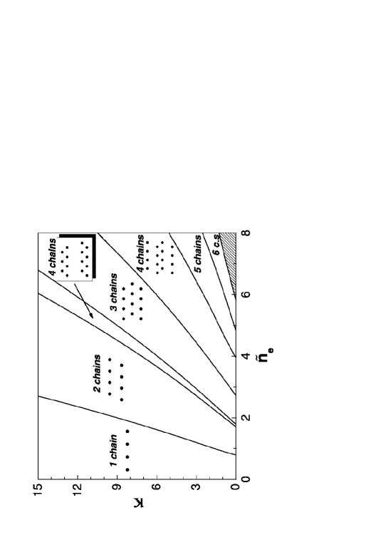
Figure 2: The zero temperature structural phase diagram.

Calculating the energy minima for different $\widetilde{n}_{e}$ and different $\kappa$ we obtain the zero temperature phase diagram of Fig. 2. For $\kappa=0$ we recover the Coulomb limit. We found that the energy obtained by the analytical method is in excellent agreement with the one obtained by our Monte Carlo simulations with a difference between them less than 0.3 %.

We observe the following sequence of transitions as the density increases : from one to the two-chain structure then to the four-chain configuration, back to the three-chain and again to four and then to five, six etc. Notice the remarkable fact that between the 2 and 3 chain configuration there is a small intermediate region where a four-chain configuration has a lower energy. For all other transitions the number of chains increases only by one unit, i.e. $n\rightarrow n+1$. The relative lateral position of the different chains are depicted in Fig. 3 as a function of the density $\widetilde{n}_{e}$. In the case of two and three-chain the inter-chain distance increases as the density increases. This is also true for the four-chain configuration too, with some differences. In the first four-chain regime of the phase diagram, the distance between the two internal chains is larger than the distance between the internal chains and the external ones, in the second regime the behavior of the system is the opposite with the distance between internal and external chains larger than the one between internal chains. For the other structures the interchain distance is always a growing function of the density. It is evident that only the first transition is continuous with a clear bifurcation.

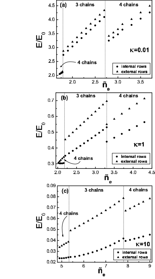
Figure 4: The energy per chain at T=0 and (a) $\kappa$=0.01, (b) $\kappa$=1 and (c)$\kappa$=10. The energy is always higher for the external chains but as the Coulomb limit ($\kappa\ll 1$) is approached the difference is diminished and the system behaves isotropically.

In order to gain some insight on the distribution of the energy in this anisotropic system we present in Fig. 4 the energy per particle for each chain. This is computed by considering a particle at a particular chain and taking into account all the interactions with the rest of the particles. The cases of interest are the configurations for which it is possible to distinguish internal from external chains and may be related to the difference in the melting behavior which is discussed in Sec. V. The interesting observation is that in every case the energy per particle is larger in the external chain than the internal ones.

This asymmetry reflects the fact that for each particle residing in an external chain the gain in energy due to the confining potential is higher than the difference in the Coulomb energy due to the lack of symmetric neighboring chains, as compared to a particle residing in an internal chain. E.g. for a three-chain system where the middle chain is the 0th and the external ones are denoted by +1 and -1, we have for the energy of two particles :

$$E_{\pm 1}-E_{0}=E_{conf,\pm 1}+E_{Coulomb,+1,-1}-E_{Coulomb,\pm 1,0}>0,$$ (7)

where E_{Coulomb,α,β} denotes the Coulomb energy of a particle residing in chain $\alpha$ interacting with the particles in chain $\beta$ and E_conf,α denotes its confining energy.

In the case of the first density regimes where the four-chain structure is optimal this difference is not large due to the fact that the internal distance is less than the external. On the contrary, the difference is much larger in the second regime of the four-chain structure. Another interesting observation is that as we approach the limit of Coulomb interactions ($\kappa\ll 1$) the energy difference tends to vanish and the system behaves isotropically.

III.2 Structural transitions

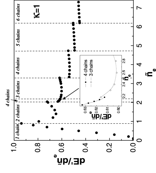
Figure 5: The derivative of the energy with respect to the density for $\kappa=1$. Only the transition from one to two-wires is continuous (second order) the rest are first order.

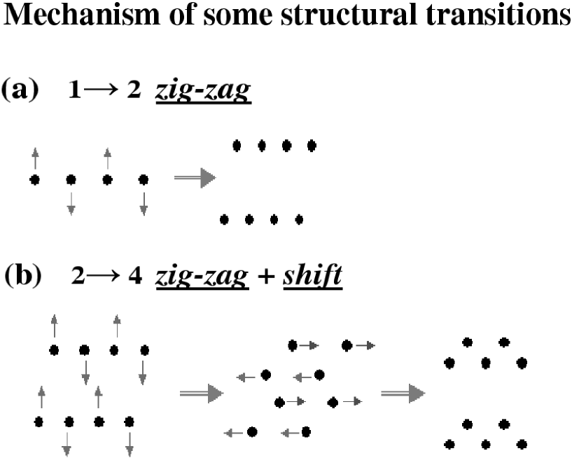
Figure 6: The mechanism of the structural transitions 1$\longrightarrow$ 2 chains and 2 $\longrightarrow$ 4 chains.

We have seen that by increasing the density, the system changes its configuration, in other words it undergoes a “structural transition”. It is a natural question to study the order of these transitions. For this purpose the derivative of the energy with respect to the density was calculated which is shown in Fig. 5 for the case of $\kappa=1$. Only the transition between the one and the two-chain configuration is continuous and all the others are discontinuous. This conclusion agrees with the results of Fig. 3 where discontinuous changes of the lateral position of the particles correspond to first order transitions. The transition $1\rightarrow 2$ is a “zig-zag”transition zigzag (Fig. 6). The transition $2\rightarrow 4$ occurs through a “zig-zag”transition of each of the two chains accompanied by a shift of $a/4$ along the chain, which makes it a weakly discontinuous transition (Fig. 6). In principle, these kind of almost “zig-zag” transitions are possible for three-, four-, five- and six- chains to result into six-, eight-, ten- and twelve- chain structures, respectively. Actually, these were observed during the numerical simulations, especially for very small value of $\kappa$, but they represent metastable states and are not the most energetically favored configurations.

III.3 Limit of short range interaction and large density

In order to make the connection with the regime where the hard core potential can be used as a working hypothesis, we investigate the limit $\lambda\ll a$. It can be shown that the variation of the distances between chains can be neglected and in the limit where $m{\omega_{0}}^{2}W^{2}\ll q^{2}/(a\epsilon)$ ($W$ is the width of the strip), following the spirit of the hydrodynamic consideration of Koulakov and Shklovskii koulakov the difference in the distance between chains at the borders $d(\pm W/2)$ and at the center $d(0)$ follows the relation:

$$\delta d_{0}=d_{0}(W/2)-d_{0}(0)\approx\lambda lnl,$$ (8)

where $l$ is the number of chains and $d_{0}=\sqrt{d^{2}+a^{2}/4}$.

This can be estimated by considering the pressure $\sigma_{yy}$ in the crystal exercised by the external potential. Adopting a method similar to Ref.koulakov ; landau :

$$\sigma_{yy}=-S(\sigma)\frac{m{\omega_{0}}^{2}}{2}(\frac{W^{2}}{4}-y^{2}),$$ (9)

where $3/4\leq S(\sigma)\leq 1$ and $\sigma$ is the Poisson ratio. We assume a uniform density $n$ and $S(\sigma)\approx 1$. Then, balancing the force by the pressure and the interaction forces we get (in this estimate we keep the dimensions for clarity):

$$\frac{2dq^{2}}{\epsilon(d^{2}+a^{2}/4)}exp(-\sqrt{d^{2}+a^{2}/4}/\lambda)\sim\frac{ndm{\omega_{0}}^{2}}{2}(W^{2}/4-y^{2}),$$ (10)

from this relation :

$$d_{0}(y)\equiv\sqrt{d(y)^{2}+a^{2}/4}\approx\lambda ln[\frac{4q^{2}}{\epsilon m{\omega_{0}}^{2}n(W^{2}/4-y^{2})(d(y)^{2}+a^{2}/4)}],$$ (11)

subtracting the values of $d_{0}$ at $W-a/2$ and 0 we obtain Eq. (6).

Therefore in the case of very short-range interaction $\delta d\ll d(0)$. Then one can adopt the hard core potential and essentially the total energy becomes the sum of the energy of each particle due to the confining potential. The average energy per unit length E/L then reads :

$$E/L\approx\frac{1}{24}m{\omega_{0}}^{2}\frac{W^{2}}{la}.$$ (12)

IV NORMAL MODES

IV.1 Normal modes in the absence of an external magnetic field

We now turn to the calculation of the normal modes of the system, following the standard harmonic approximation pines and exploiting the translational invariance of the system along the $x$ direction. The number of chains determines the number of particles in each unit cell and therefore the number of degrees of freedom per unit cell. So if $l$ is the number of chains there will be $2l$ branches for the normal mode dispersion curves: $l$ acoustical branches as well as $l$ optical ones. Note that for ordinary bidimensional crystals there are 2 acoustical branches and $2r-2$ optical branches, if $r$ is the number of atomic species in the unit cell. We present the results for the one, two and three-chain structure in Fig. 7. Note that for the one chain structure the unit cell consists of a single particle, i.e. $r=1$, and therefore one expects only a single acoustical branch and no optical branch. The appearance of the optical branch is a consequence of the presence of the confining potential in the $y$-direction. Note that for $k\rightarrow 0$, $\omega_{opt}\approx\omega_{0}$, which corresponds to the center of mass motion of the system in the confining potential.

In order to find the eigenmodes we solve the system of equations :

$$(\omega^{2}\delta_{\alpha\beta,ij}-D_{\alpha\beta,ij})Q_{\beta,j}=0,$$ (13)

where $Q_{\beta,j}$ is the displacement of the particle $j$ from its equilibrium position in the $\beta$ direction, $(\alpha,\beta)\equiv{(x,y)}$, $\delta_{\alpha\beta,ij}$ is a unit matrix and $D_{\alpha\beta,ij}$ is the dynamical matrix defined by:

$$D_{\alpha\beta,ij}=\frac{1}{m}\sum_{\nu}\phi_{\alpha,\beta}(\nu)e^{-i\nu qa}$$ (14)

where $\nu$ is an integer assigned to each unit cell and the force constants are :

$$\phi_{\alpha,\beta}(\nu)=\partial_{\alpha}\partial_{\beta}\frac{exp(-\kappa\sqrt{(x-x^{\prime})^{2}+(y-y^{\prime})^{2}}}{\sqrt{(x-x^{\prime})^{2}+(y-y^{\prime})^{2}}},\;\;\nu\neq 0,$$ (15)

evaluated at $x-x^{\prime}\in\{a\nu,a(\nu+1/2)\}$, $y-y^{\prime}=$ relevant interchain distance. And

$$\phi_{\alpha,\beta}(\nu=0)=-\sum_{\nu\neq 0}\phi_{\alpha,\beta}(\nu).$$ (16)

All the frequencies are measured in unit of $\omega_{0}/\sqrt{2}$. In Appendix B we present for completeness the expressions for the matrix where as an example the modes for the three-chain structure were calculated.

The main feature is the softening of the optical mode of the one chain structure at the values of $\widetilde{n}_{e}$ and $\kappa$ where the structural transition is observed (“zig-zag” transition) accompanied by a hardening of the acoustical branch (Fig. 8), which confirms that $1\rightarrow 2$ is a continuous transition as asserted before.

Studying the eigenvectors of the dynamical matrix it is easy to recognize that the optical modes are identified with the motion in the direction of confinement ($y$ direction) while the acoustical modes are identified with the motion in the unconfined $x$ direction.

The eigenfrequencies for the single chain are given by : $\omega_{ac}=\sqrt{A_{1}}$ for the acoustical branch and $\omega_{opt}=\sqrt{1+A_{2}}$ for the optical branch, where $A_{1}$ and $A_{2}$ are defined in Appendix B.

In the limit of small wavenumbers $k$, the summations can be done analytically and we obtain:

$$\omega_{ac}(k) = [-ln(1-e^{-\kappa/\widetilde{n}_{e}})+\frac{\kappa}{\widetilde{n}_{e}}\frac{e^{-\kappa/\widetilde{n}_{e}}}{1-e^{-\kappa/\widetilde{n}_{e}}}+\frac{{\kappa}^{2}}{2{\widetilde{n}_{e}}^{2}}\frac{e^{-\kappa/\widetilde{n}_{e}}}{(1-e^{-\kappa/\widetilde{n}_{e}})^{2}}]^{1/2}{\widetilde{n}_{e}}^{3/2}|k|a,$$ (17)

$$\omega_{opt}(k) = \{1-[-ln(1-e^{-\kappa/\widetilde{n}_{e}})+\frac{\kappa}{\widetilde{n}_{e}}\frac{e^{-\kappa/\widetilde{n}_{e}}}{1-e^{-\kappa/\widetilde{n}_{e}}}]{\widetilde{n}_{e}}^{3}k^{2}a^{2}\}^{1/2},$$ (18)

which gives explicitly the dependence of the modes on the density and the screening parameter. In the limit $\kappa/\widetilde{n}_{e}\gg 1$ :

$$\omega_{ac}(k) = e^{-\kappa/\widetilde{n}_{e}}\frac{{\kappa}^{2}}{2\sqrt{\widetilde{n}_{e}}}|k|a,$$ (19)

$$\omega_{opt}(k) = 1-e^{-\kappa/\widetilde{n}_{e}}\frac{{\widetilde{n}_{e}}^{2}}{2\kappa}k^{2}a^{2},$$ (20)

while in the opposite limit $\kappa/\widetilde{n}_{e}\ll 1$ :

$$\omega_{ac}(k) = [\frac{3}{2}+ln(\frac{\widetilde{n}_{e}}{\kappa})]^{1/2}{\widetilde{n}_{e}}^{3/2}|k|a,$$ (21)

$$\omega_{opt}(k) = \{1-[1+ln(\frac{\widetilde{n}_{e}}{\kappa})]{\widetilde{n}_{e}}^{3}k^{2}a^{2}\}^{1/2}.$$ (22)

There is a remarkable difference in the optical branch of the spectrum between the single chain and the two and three-chain structures. In the first case the frequency of the optical branch decreases as the wavenumber $k$ increases, while for the two and three-chain structures the optical frequency increases. In the single chain configuration the optical mode corresponds to oscillations of the particles in the confined direction (see e.g. Fig. 9(b)) which reduces the Coulomb repulsive energy. For the two chain configuration the normal modes are shown in Fig. 9(c-g). In fact this branch is nothing else than a transverse acoustical mode while the acoustical branch corresponds to longitudinal motion kovdrya ; sokolov .

IV.2 Normal modes in the presence of an external magnetic field

We now consider the effect of applying a constant magnetic field $B$ in the $z$ direction. For quantum particles, the magnetic field can localize the charged particles into cyclotron orbits, therefore aiding the formation of a Wigner crystal in the presence of a magnetic field. It is known vanlee that in a classical system an external magnetic field does not alter the statistical properties of the system and consequently the structural properties and the melting temperature are insensitive to the magnetic field strength. But on the other hand the character of motion of the particles is altered significantly when the cyclotron frequency is larger than the eigenfrequencies of the system. The magneto-phonon spectrum of an infinite 2D Wigner crystal in a magnetic field was obtained in chaplik , bonsall . In the presence of $B$, the system of equations is modified to:

$$(\omega^{2}\delta_{\alpha\beta,ij}-D_{\alpha\beta,ij}+i\omega\omega_{c}\xi_{\alpha\beta}\delta_{ij})Q_{\beta,j}=0$$ (23)

where $\xi_{\alpha\beta}$ is the Levi-Civita tensor and $\omega_{c}=qB/mc$ is the cyclotron frequency. In Fig. 10 we show some typical dispersion curves for the one and three-chain structures for different values of $\omega_{c}$. It is interesting to notice how the optical modes couple with the magnetic field, the optical frequencies follow the cyclotron frequency and for very high field strength there is no significant difference between $\omega_{opt}$ and $\omega_{c}$. The acoustical frequencies on the other hand decrease with the magnetic field strength. For the single chain the eigenfrequencies are modified to:

$$\omega(k)=\{\frac{1}{2}(1+A_{1}+A_{2}+{\omega_{c}}^{2})\pm\frac{1}{2}[(1+A_{1}+A_{2}+{\omega_{c}}^{2})^{2}-4A_{1}(1+A_{2})]^{1/2}\}^{1/2}$$ (24)

where $A_{1}$ and $A_{2}$ are given in Appendix B. For very large field when $\omega_{c}\gg$ {$A_{1}$,$A_{2}$,1} the gap between the optical branches and the acoustical ones approaches $\omega_{c}$. The optical frequency reflects the cyclotron motion of the system which supresses any soft excitation. As before, it is interesting to study the normal modes at the critical density of the transition from the one-chain to the two-chain structure (Fig. 11). We observe that there is always softening at the same density, independently of the strength of the magnetic field, but with a main difference that for zero magnetic field strength the modes which soften is the optical one while when the magnetic field strength is nonzero, the acoustic mode is the one that softens. The magnetic field induces a coupling between the acoustical and the optical modes and there is an anticrossing between the two branches. Although these findings confirm the previous assertion that the presence of $B$ does not alter the structural properties of the system it also reveals the differences (softening of the acoustic mode at the same density, influence on the gap between optical and acoustical branches and on eigenfrequencies within each branch) which are induced by the magnetic field.

V MELTING

V.1 General discussion and results

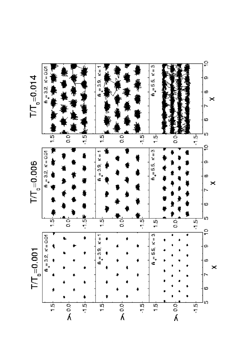
Figure 12: Particle trajectories for $3\times 10^{7}$ MC steps for three different temperatures and three different values of the density at $\kappa$ = 1.

In this section we study the melting of the WC by MC simulations. After the ground state configuration was achieved as explained in Sec. II, the system was heated up by steps of size $\Delta T$, typically $\Delta T=5\times 10^{-4}$, and equilibrated to this new temperature during $10^{5}\div 10^{6}$ MC steps. In Fig. 12 we show typical trajectories of particles as they arise from our MC simulation. It is evident that there is a different behavior of the system in the $x$ and the $y$ directions as may be expected by the anisotropy in the two directions. In order to quantify the observations, we studied first the potential energy as a function of temperature (Fig. 13). In the crystalline state the potential energy of the system increases practically linearly with temperature and then exhibits a very fast increase in a small critical temperature range after which it starts to increase linearly again but now with a slightly larger slope. In the latter region the system is in the disordered ($i.e.$ liquid) phase. The fast increase of the potential energy is indicative of the melting of the WC. To find the critical temperatures we studied, following the spirit of Ref. bedanov , the modified Lindemann parameter $L_{p}=\langle u^{2}\rangle/{d_{r}}^{2}$, where $\langle u^{2}\rangle$ is defined by the difference in the mean square displacements of neighboring particles from their equilibrium sites $\vec{r}_{0}$ and $d_{r}$ is the relevant interparticle distance as we discuss below. The quantity $\langle u^{2}\rangle$ can be written as:

$$\langle u^{2}\rangle=\frac{1}{N}\langle\underset{i=1}{\overset{N}{\sum}}\frac{1}{N_{nb}}\underset{j=1}{\overset{N_{nb}}{\sum}}[(\vec{r}_{i}-\vec{r}_{0i})-(\vec{r}_{j}-\vec{r}_{0j})]^{2}\rangle$$ (25)

where $\langle$ $\rangle$ means the average over the MC steps, $N$ is the total number of particles in our simulation unit cell and the index $j$ denotes the $N_{nb}$ nearest neighbors of particle $i$. In order to describe more accurately the difference between the two directions, we studied separately $\langle u_{x}^{2}\rangle$ and $\langle u_{y}^{2}\rangle$ as function of temperature. For the melting along the $x$ direction, the distance $d_{r}$ is the interparticle distance $a$ introduced in Sec. I while for melting along the $y$ direction $d_{r}$ is the interchain distance which is a function of the density $\widetilde{n}_{e}$.

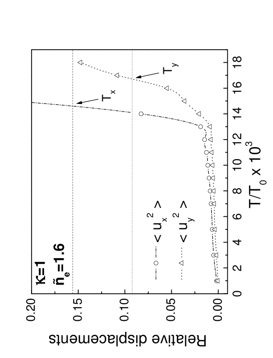
Figure 14: The mean square relative displacements for $\kappa$= 1, $\widetilde{n}_{e}$= 1.6 in the case of the two-chain configuration. The dashed horizontal line corresponds to the modified Lindemann criterion (MLC) in the unconfined direction, while the dotted line corresponds to the MLC in the confined direction.

At low temperatures, the mean square relative displacements slowly increases linearly with temperature as a consequence of harmonic oscillations of the particles about their equilibrium positions (see Fig. 14). From Fig. 14 we notice clearly that this linear increase is larger in the unconfined direction than in the confined direction. In some critical temperature region, $\langle u_{x}^{2}\rangle$ and $\langle u_{y}^{2}\rangle$ start to increase very rapidly which is the consequence of the fact that the particles have attained sufficient thermal energy that they can jump between different crystallographic positions. According to the modified Lindemann criterion MLC, when $L_{p}$ reaches the (semi-empirical) critical value 0.1 the system melts. This criterion was used to define the melting temperature $T_{m}$.

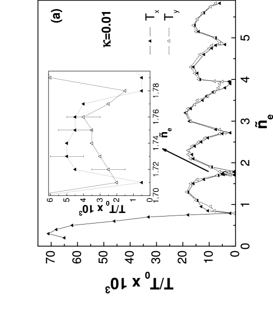
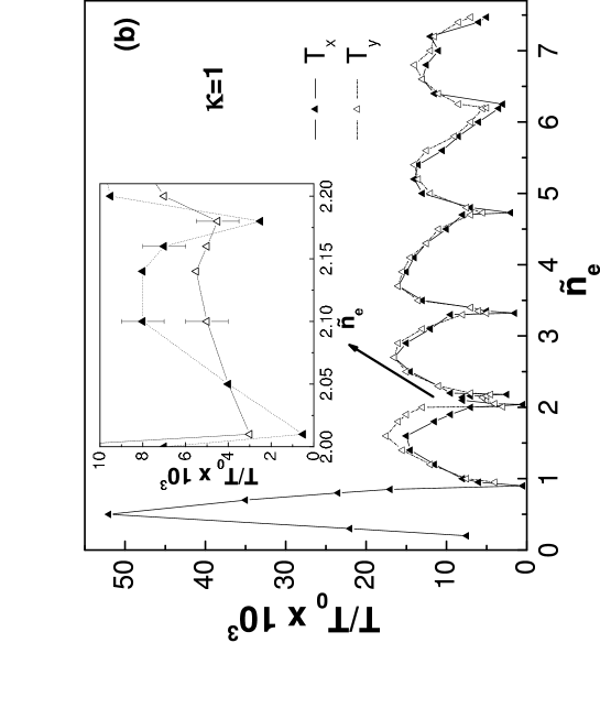
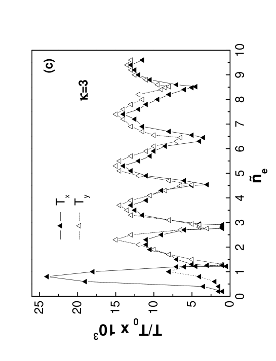
Figure 15: Melting temperature as a function of density for: (a) $\kappa$ = 0.01, (b) $\kappa$=1, and (c) $\kappa=3$. The insets in (a) and (b) show an enlargement of the four-chain region which is located between the two and three chain phase.

From the corresponding analysis two different melting temperatures, $T_{x}$ and $T_{y}$, can be assigned. The results are summarized in the phase diagram of Figs. 15(a-c) for $\kappa=$0.01, 1 and 3, respectively. There are several interesting features in these phase diagrams: ($a$) the nearly Coulomb system ($\kappa=0.01$) has a melting temperature which is on average 15-20 % higher than for the screened Coulomb inter-particle interaction with $\kappa=1$, which has on its turn an average melting temperature about 15 % higher than the screened Coulomb system with $\kappa=3$. Therefore, we conclude that the effect of screeening is to reduce the melting temperatures ; ($b$) a reentrant behavior is observed as a function of density, the minima of the melting temperatures occur at the values of the density where the structural phase transitions were predicted (see Fig. 2); ($c$) there is a regime close to each structural transition point where the system is frustrated, in the sense that it fluctuates between the two structures. In this regime, which we term as frustration regime, the system makes continuous transitions from one metastable state to the other which strongly reduces the melting temperature; ($d$) for $\kappa=1$ and $\kappa=3$, there is a region in density for which the system melts first in the unconfined direction while it is not melted in the confined one. This regime resembles the findings of Ref. radzihovsky in the regime termed as locked floating solid. For the Coulomb limit there is no evidence of anisotropic melting within the error bars of our simulation. The system behaves more isotropic; ($e$) the first four-chain regime (see insets of Figs. 15a-c) is unstable with respect to temperature fluctuations as it is reflected in the relative low melting temperature. In this region, melting occurs first in the confined direction as a consequence of the particular structural properties -the distance between the two internal chains is larger than the distance between an internal chain and the adjacent external one- which makes the system unstable in the $y$ direction. In the rest of the diagram there is evidence that the melting either starts from the unconfined direction (e.g. it is clear in the single chain and in the low density limit of the two-chains) or the system melts simultaneously in both directions. ($f$) the single-chain structure shows a relatively large melting temperature as obtained by the MLC and deserves more attention. The study of the single-chain is therefore postponed to the next subsection.

Furthermore, note that the MLC only takes into account the displacement of the particles relative to the position of their neighbors and consequently is only a measure of the local order of the system.

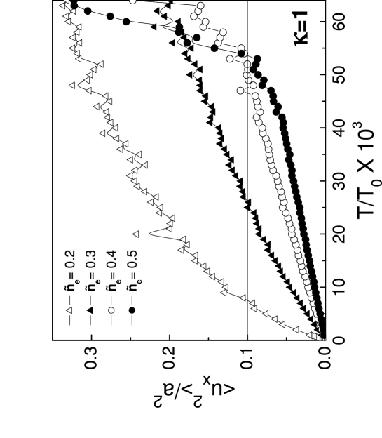
Figure 18: The behavior of the Lindemann parameter, for the single-chain regime at four different densities. It shows how the linear regime at higher densities becomes sublinear at lower densities.

Another natural question that arises is whether there is anisotropic melting with respect to external and internal chains in the multi-chain structures or in other words if melting starts from the edges as observed in the experiment of Ref. glasson with electrons on liquid helium. The number of filaments that were observed in the experiment was approximately 20; we have simulated the trajectories of some multi-chain structures and the results are presented in Fig. 18. In this picture it is clear that the most external chains are already melted while the internal ones are still ordered. Edge melting has also been demonstrated in the presence of a strong magnetic field in Ref. cote using Hartree-Fock calculations in a two-dimensional Wigner crystal with edges. With the aid of many numerical simulations of multi-chain systems at different densities we observed that this kind of melting is present in our system when the density is close enough to the critical density of a structural transition. Close to the structural transition many metastable states appear with a different number of particles per chain, that is in the most external chains there are less particles than in the internal ones. Thus the particles at the most external chains have larger displacements from their equilibrium positions in order to attain the stability of the structure. Furthermore, we calculated the average root mean square displacements of the particles from their equilibrium position chain by chain and also $\langle u_{x}^{2}\rangle$ chain by chain and we actually noted that these quantities are slightly larger for external chains at temperatures

below the critical one. In Fig. 19 we present the temperature dependence of the standard deviation ${s_{x}}^{2}=\langle(u_{x}-\langle u_{x}\rangle)^{2}\rangle$ and ${s_{x}}^{2}=\langle(u_{y}-\langle u_{y}\rangle)^{2}\rangle$ for the external and internal chains in the four-chain structure. It is evident that the position of the particles at the edges fluctuates substantially more than the particles at the interior. We can conjecture that, according to this physical picture, melting can start from the edges. However, for up to the six-chain configuration for each chain the quantities $\langle u_{x}^{2}\rangle$ reached the critical value, approximately, all at the same temperature. Probably, going to a larger number of filaments one can well appreciate a different melting temperature for external and internal chains. Finally, the chain configuration as well as the melting which starts from the direction of the chains is supported also by molecular dynamics simulations of the flow of electrons in Q1D channels mehrotra .

V.2 Melting of the single-chain

In Figs. 15(a-c) we observe a rather high melting temperature in case of the one-chain structure. The origin of this behavior can be traced back to the fact that the MLC takes into account a larger contribution from jumps of particles between crystallographic positions which for the single chain structure occurs only at extremely high temperature. For the single-chain case the jumps can only occur along the chain which requires a larger energy than jumps of particles between different chains.

To have a better insight we investigated the behavior of $L_{p}$ for different densities (Fig. 18). We notice that in the low density limit (see Fig. 18(a)), $L_{p}$ $\approx$ 0.1 is reached in a region in which there is only a gradual increase in $\langle u_{x}^{2}\rangle$ which is very different from the multi-chain case (see Fig. 14). Furthermore, $\langle u_{x}^{2}\rangle$ exhibits a sublinear temperature increase.

This calls for the use of other possible criteria in order to clarify the situation. On the other hand if the density is relatively high (see Fig. 18), a fast increase is observed signaling a clear melting of the system. The transition from a low temperature linear to sublinear behaviour occurs for $\widetilde{n}_{e}\approx 0.4$.

To shine light into the posed questions we studied also the pair correlation function at different densities and temperatures, as defined by

$$g(x)=\frac{L}{N^{2}}\sum_{i\neq j}<\delta[x-(x_{i}-x_{j})]>,$$ (26)

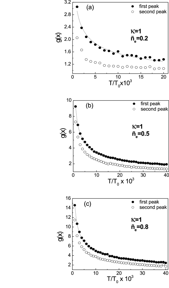
Figure 20: The height of the first and second peaks of the pair correlation function for the single chain as a function of temperature for three different densities.The lines are the best fits with the function $\alpha(T/T_{0})^{-\beta}$.

where in the summation over $N$ particles in a system of length $L$, the diagonal terms ($i=j$) are excluded . The results are reported in Fig. 19. It is rather evident that the melting temperature is substantially smaller than the one obtained from the MLC. In order to better quantify the melting temperature for the one-chain structure we investigated the height of the first and second peak of the pair correlation function as function of temperature (see Fig. 20) in order to look for a structure or an anomalous jump (as found in Ref. vsch ) that could identify the critical temperature. As is apparent from Fig. 20 we do not find any abrupt changes. The first and second peak as a function of temperature can be fitted by : $g_{i}=\alpha(T/T_{0})^{-\beta}$, where $i=\{1$ or $2\}$ denotes the peak (see the curves in Fig. 20).

The values of ($\alpha$,$\beta$) are (2.922, 0.274) for $i=1$ and (1.895, 0.216) for $i=2$ when $\widetilde{n}_{e}=0.2$, (9.320, 0.433) for $i=1$ and (7.345, 0.466) for $i=2$ when $\widetilde{n}_{e}=0.5$, (14.788, 0.473) for $i=1$ and (11.552, 0.501) for $i=2$ when $\widetilde{n}_{e}=0.8$ and in each case the error is less than $1\%$.

From the study of the pair correlation function we conclude that at moderate ($\tilde{n}_{e}\leq 0.2$ for $\kappa=1$) densities, the chain is melted at arbitrarily weak temperature. For higher densities the chain retains correlations up to higher values of the temperature but these values are less than those obtained by the MLC.

We noticed from the high density regime ($\widetilde{n}_{e}>1$), where we reach the multichain structure, that another semi-empirical criterion can be formulated using the pair correlation function. If we consider the ratio of the height of the fifth peak in $g(x)$ above 1 ($H_{5}-1$) to the height of the first peak above 1 ($H_{1}-1$) at those densities where the maximum melting temperature is obtained for the two, three and four chain structures, melting occurs when :

$$\frac{H_{5}-1}{H_{1}-1}(T_{m})\approx 0.15$$ (27)

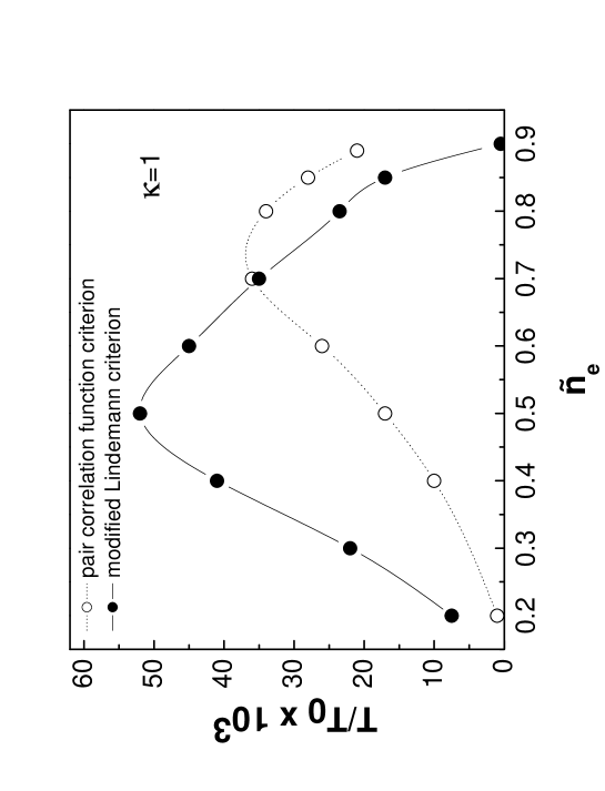
Figure 21: The melting temperature for the single chain as obtained from the two complementary criteria.

Employing this criterion (termed as pair correlation function criterion or PCFC) we obtain the results of Fig. 21, were we present both the relevant temperatures obtained by MLC and PCFC.

It is worth noticing that this criterion does not work well at temperatures close to the structural transitions. The reason is that although particles “jump” to new sites in order to attain the new positions, the pair correlation function still measures correlations at certain distances and, most importantly, the height of the first peak is substantially reduced which artificially enhances the ratio (25).

Thus the value of $15\%$ which works far from the structural transitions is too high for the regime close to the structural transitions. It is therefore evident that the two criteria can work in a complementary manner.

VI DISCUSSION AND CONCLUSIONS

The structural phase transitions and the melting can be studied experimentally using parabolically confined colloidal particles or dusty plasmas in the case of a screened Coulomb inter-particle interaction. Another important experimental system are electrons floating on liquid helium where it is possible to achieve relatively narrow Q1D channels on very stable suspended helium films over structured substrates sokolov . Assuming a semicircular profile of the liquid surface across the channels then the confining potential is parabolic near the bottom with $\omega_{0}=(eE_{\perp}^{*}/mR)$ sokolov where $E_{\perp}^{*}$ is the effective holding electric field in the case of the substrate and R the radius of the semicircular profile. Assuming a radius of approximately 5 $\mu m$, a typical value for $E_{\perp}^{*}\approx 10kV/cm$ then $\omega_{0}$ $\approx 10^{11}$ Hz. This in turn produces a $T_{0}\approx 60K$. The melting temperatures which have been obtained in the present work are of order $10^{-2}\times T_{0}$ which results in a melting temperature $\approx 0.5-1K$, a temperature range which is routinely achieved in such experiments. Assuming an interelectron distance of approximately 0.1 - 1 $\mu m$ leads to a dimensionless linear density ${\tilde{n}}_{e}\approx(0.5-3)l$, where $l$ is the number of chains. The dilute limit gives the same ${\tilde{n}}_{e}$ as the one investigated in the present work.

Another issue connected with melting, which deserves interest, is the appearance of topological defects so that a KTHNY kthny scenario of melting is possible. In Ref.koulakov ; bedanov ; kong this question was considered in the case of a circular confining potential with a finite number of particles. In the case of short range interactions the defects are pushed to the surface due to the large price for elastic deformations while in the Coulomb case shear and Young moduli are relatively small koulakov .

Moreover, because of the incommensurability of the circle with the hexagonal Wigner crystal the defects do not reside exactly at the borders but in a zone few lattice spacings inside the crystal. Therefore three different regimes with different melting temperatures can be detected kong . In our case there is no such incommensurability and the edges can accommodate the defects easily. This has also been discussed in the case of a quantum Hall bar by Nazarov in Ref.nazarov .

In conclusion, we investigated the structural, dynamical properties and melting of a classical quasi-1D system of particles interacting through a Yukawa-type potential in the range from Coulomb to very short range interaction in the case where the confinement is modelled by an external parabolic potential. The structural transitions are of first (primarily) and second order. The normal modes of the system were calculated in the presence of a perpendicular magnetic field. In certain regions of the parameter space, there is evidence that melting starts first in the unconfined direction before the system melts along the chain direction. Furthermore, we found that $T_{m}$ shows a reentrant behavior as a function of the density of the system and a regime of frustration around each point of structural transition can be identified. In the case of the single chain structure, we device a new criterion in order to take into account the correlations at different temperatures. The present study is suitable to describe colloidal particles, dusty plasmas and electrons floating on liquid helium.

VII APPENDIX A

The expressions for the energy in the configurations beyond the two-chain structure are presented below. All the distances are in units of the interchain distance $a$ between adjacent particles.

For the three-chain structure :

$$E_{3}=\frac{\widetilde{n}_{e}}{3}\sum_{m=1}^{\infty}exp(-3m\kappa/\widetilde{n}_{e})/m+\frac{4\widetilde{n}_{e}}{9}\sum_{m=1}^{\infty}\frac{exp(-3\kappa\sqrt{(m-1/2)^{2}+{c_{3}}^{2}}/\widetilde{n}_{e})}{\sqrt{(m-1/2)^{2}+{c_{3}}^{2}}}$$

$$+\frac{2\widetilde{n}_{e}}{9}\sum_{m=1}^{\infty}\frac{exp(-3\kappa\sqrt{m^{2}+4{c_{3}}^{2}}/\widetilde{n}_{e})}{\sqrt{m^{2}+4{c_{3}}^{2})}}+6\frac{{c_{3}}^{2}}{{\widetilde{n}_{e}}^{2}}+\frac{\widetilde{n}_{e}exp(-6c_{3}\kappa/\widetilde{n}_{e})}{18c_{3}},$$ (28)

where the intrachain distance $c_{3}$ is a variational parameter.

For the four-chain structure :

$$E_{4} = \frac{\widetilde{n}_{e}}{4}\sum_{m=1}^{l}\frac{exp(-4\kappa m/\widetilde{n}_{e})}{m}+\frac{\widetilde{n}_{e}}{4}\sum_{m=1}^{\infty}\frac{exp(-4\kappa\sqrt{(m-1/2)^{2}+(c_{4}-f_{4})^{2}}/\widetilde{n}_{e})}{\sqrt{(m-1/2)^{2}}+(c_{4}-f_{4})^{2}}$$ (29)

$$+ \frac{\widetilde{n}_{e}}{4}\sum_{m=1}^{\infty}\frac{exp(-4\kappa\sqrt{(m^{2}+(c_{4}+f_{4})^{2}}/\widetilde{n}_{e})}{\sqrt{m^{2}+(c_{4}+f_{4})^{2}}}+\frac{\widetilde{n}_{e}}{8}\sum_{m=1}^{\infty}\frac{exp(-4\kappa\sqrt{(m-1/2)^{2}+4{f_{4}}^{2}}/\widetilde{n}_{e})}{\sqrt{(m-1/2)^{2}+4{f_{4}}^{2}}}$$

$$+ \frac{\widetilde{n}_{e}}{8}\sum_{m=1}^{\infty}\frac{exp(-4\kappa\sqrt{(m-1/2)^{2}+4{c_{4}}^{2}}/\widetilde{n}_{e})}{\sqrt{(m-1/2)^{2}+4{c_{4}}^{2}}}+\frac{8{c_{4}}^{2}}{{\widetilde{n}_{e}}^{2}}+8{f_{4}}^{2}/{\widetilde{n}_{e}}^{2}$$

$$+ \frac{\widetilde{n}_{e}}{8}\frac{exp[-4(c_{4}+f_{4})\kappa/\widetilde{n}_{e}]}{c_{4}+f_{4}},$$

where $c_{4}$ is the distance of an inner chain and $f_{4}$ is the distance of an outer chain from the middle of the structure. These distances are two variational parameters which have to be optimized numerically.

For the five-chain structure :

$$E_{5} = \frac{10{c_{5}}^{2}}{{\widetilde{n}_{e}}^{2}}+\frac{10{f_{5}}^{2}}{{\widetilde{n}_{e}}^{2}}+\frac{\widetilde{n}_{e}}{5}\sum_{m=1}^{\infty}\frac{exp(-5\kappa m/\widetilde{n}_{e})}{m}+\frac{4\widetilde{n}_{e}}{25}\sum_{m=1}^{\infty}\frac{exp(-5\kappa\sqrt{(m-1/2)^{2}+(c_{5}-f_{5})^{2}}/\widetilde{n}_{e})}{\sqrt{(m-1/2)^{2}+(c_{5}-f_{5})^{2}}}$$ (30)

$$+ \frac{4\widetilde{n}_{e}}{25}\sum_{m=1}^{\infty}\frac{exp(-5\kappa\sqrt{m^{2}+{c_{5}}^{2}}/\widetilde{n}_{e})}{\sqrt{m^{2}+{c_{5}}^{2}}}+\frac{2\widetilde{n}_{e}}{25}\frac{exp(-5c_{5}\kappa/\widetilde{n}_{e})}{c_{5}}+\frac{4\widetilde{n}_{e}}{25}\sum_{m=1}^{\infty}\frac{exp(-5\kappa\sqrt{(m-1/2)^{2}+(c_{5}+f_{5})^{2}}/\widetilde{n}_{e})}{\sqrt{(m-1/2)^{2}+(c_{5}+f_{5})^{2}}}$$

$$+ \frac{2\widetilde{n}_{e}}{25}\sum_{m=1}^{\infty}\frac{exp(-5\kappa\sqrt{m^{2}+4{c_{5}}^{2}}/\widetilde{n}_{e})}{\sqrt{m^{2}+4{c_{5}}^{2}}}+\frac{\widetilde{n}_{e}}{50}\frac{exp(-10c_{5}\kappa/\widetilde{n}_{e})}{c_{5}}+\frac{4\widetilde{n}_{e}}{25}\sum_{m=1}^{\infty}\frac{exp(-5\kappa\sqrt{(m-1/2)^{2}+{f_{5}}^{2}}/\widetilde{n}_{e})}{\sqrt{(m-1/2)^{2}+{f_{5}}^{2}}}$$

$$+ \frac{2\widetilde{n}_{e}}{25}\sum_{m=1}^{\infty}\frac{exp(-5\kappa\sqrt{m^{2}+4{f5}^{2})/\widetilde{n}_{e}})}{\sqrt{m^{2}+4{f_{5}}^{2}}}+\frac{\widetilde{n}_{e}exp(-10f_{5}\kappa/\widetilde{n}_{e})}{50f_{5}},$$

with the variational parameters $c_{5}$ and $f_{5}$, which are the distance of an inner chain and outer chain respectively from the middle of the structure.

For the six-chain structure :

$$E_{6} = \frac{12{f_{6}}^{2}}{{\widetilde{n}_{e}}^{2}}+\frac{12{g_{6}}^{2}}{{\widetilde{n}_{e}}^{2}}+\frac{12{h_{6}}^{2}}{{\widetilde{n}_{e}}^{2}}+\frac{\widetilde{n}_{e}}{6}\sum_{m=1}^{\infty}\frac{exp(-6\kappa m/6)}{m}+\frac{\widetilde{n}_{e}}{18}\sum_{m=1}^{\infty}(\frac{exp(-6\kappa\sqrt{(m-1/2)^{2}+4{h_{6}}^{2}}/\widetilde{n}_{e})}{\sqrt{(m-1/2)^{2}+4{h_{6}}^{2})}}$$ (31)

$$+ \frac{\widetilde{n}_{e}}{18}\sum_{m=1}^{\infty}(\frac{exp(-6\kappa\sqrt{(m-1/2)^{2}+4{f_{6}}^{2}}/\widetilde{n}_{e})}{\sqrt{(m-1/2)^{2}+4{h_{6}}^{2})}}+\frac{\widetilde{n}_{e}}{18}\sum_{m=1}^{\infty}(\frac{exp(-6\kappa\sqrt{(m-1/2)^{2}+4{g_{6}}^{2}}/\widetilde{n}_{e})}{\sqrt{(m-1/2)^{2}+4{g_{6}}^{2}}})$$

$$+ \frac{\widetilde{n}_{e}}{9}\sum_{m=1}^{\infty}\frac{exp(-6\kappa\sqrt{(m-1/2)^{2}+(h_{6}-g_{6})^{2}}/\widetilde{n}_{e})}{\sqrt{(m-1/2)^{2}+(h_{6}-g_{6})^{2}}}+\frac{\widetilde{n}_{e}}{9}\sum_{m=1}^{\infty}\frac{exp(-6\kappa\sqrt{(m-1/2)^{2}+(h_{6}+f_{6})^{2}}/\widetilde{n}_{e})}{\sqrt{(m-1/2)^{2}+(h_{6}+f_{6})^{2})}}$$

$$+ \frac{\widetilde{n}_{e}}{9}\sum_{m=1}^{\infty}\frac{exp(-6\kappa\sqrt{(m-1/2)^{2}+(g_{6}-f_{6})^{2}}/\widetilde{n}_{e})}{\sqrt{(m-1/2)^{2}+(g_{6}-f_{6})^{2})}}+\frac{\widetilde{n}_{e}}{9}\sum_{m=1}^{\infty}\frac{exp(-6\kappa\sqrt{m^{2}+(h_{6}-f_{6})^{2})}/\widetilde{n}_{e})}{\sqrt{m^{2}+(h_{6}-f_{6})^{2}}}$$

$$+ \frac{\widetilde{n}_{e}}{18}\frac{exp(-6|h_{6}-f_{6}|\kappa/\widetilde{n}_{e})}{{|h_{6}-f_{6}|}}+\frac{\widetilde{n}_{e}}{9}\sum_{m=1}^{\infty}\frac{exp(-6\kappa\sqrt{m^{2}+(h_{6}+g_{6})^{2}}/\widetilde{n}_{e})}{\sqrt{m^{2}+(h_{6}+g_{6})^{2}}}+\frac{\widetilde{n}_{e}}{18}\frac{exp[-6(h_{6}+g_{6})\kappa/\widetilde{n}_{e}]}{{(h_{6}+g_{6})}}$$

$$+ \frac{\widetilde{n}_{e}}{9}\sum_{m=1}^{\infty}\frac{exp(-6\kappa\sqrt{m^{2}+(g_{6}+f_{6})^{2}}/\widetilde{n}_{e})}{\sqrt{m^{2}+(g_{6}+f_{6})^{2}}}+\frac{\widetilde{n}_{e}}{18}\frac{exp[-6(g_{6}+f_{6})\kappa/\widetilde{n}_{e}]}{(g_{6}+f_{6})},$$

with $f_{6}$, $g_{6}$ and $h_{6}$ the three chain distances from the middle of the crystal, starting from the inner one which are the variational parameters.

VIII APPENDIX B

We present the matrix $\omega^{2}{\bf I}-{\bf D}$ where ${\bf I}$ is the unit matrix and ${\bf D}$ is the dynamical matrix, for the calculation of the normal modes for the three-chain structure. It reads :

$$\omega^{2}{\bf I}-{\bf D}=\begin{pmatrix}{\omega}^{2}-A_{1}&0&-A_{3}&0&-A_{5}&0\\ 0&({\omega}^{2}-{\omega_{0}}^{2})-A_{2}&0&-A_{4}&0&-A_{6}\\ -A_{3}&0&{\omega}^{2}-A_{1}&0&-A_{3}&0\\ 0&-A_{4}&0&({\omega}^{2}-{\omega_{0}}^{2})-A_{2}&0&-A_{4}\\ -A_{5}&0&-A_{3}&0&{\omega}^{2}-A_{1}&0\\ 0&-A_{6}&0&-A_{4}&0&({\omega}^{2}-{\omega_{0}}^{2})-A_{2}\end{pmatrix}\quad$$ (32)

where the parameters are :

$$A_{1} = {\tilde{n}_{e}}^{3}\sum_{j=1}^{\infty}\frac{1}{27j^{3}}exp(-3j\kappa/{\tilde{n}_{e}})[2+6j\kappa/\tilde{n}_{e}+9j^{2}{\kappa}^{2}/{\tilde{n}_{e}}^{2}](1-cos(\tilde{k}\pi j)),$$

$$A_{2} = -{\tilde{n}_{e}}^{3}\sum_{j=1}^{\infty}\frac{1}{27j^{3}}exp(-3j\kappa/{\tilde{n}_{e}})(2+3j\kappa/\tilde{n}_{e})(1-cos(\tilde{k}\pi j)),$$

$$A_{3} = {\tilde{n}_{e}}^{3}\sum_{j=1}^{\infty}\frac{1}{27\sqrt{(j+1/2)^{2}+c^{2}}}exp(-3\kappa\sqrt{(j+1/2)^{2}+c^{2}}/\tilde{n}_{e})[cos(\tilde{k}\pi(j+1/2))-1](j+1/2)^{2}\times$$

$$[\frac{9\kappa\sqrt{(j+1/2)^{2}+{c_{3}}^{2}}}{\tilde{n}_{e}}+\frac{9{\kappa}^{2}[(j+1/2)^{2}+{c_{3}}^{2}]}{{\tilde{n}_{e}}^{2}}+3]-(1+\frac{3\kappa\sqrt{(j+1/2)^{2}+c^{2}}}{\tilde{n}_{e}})[(j+1/2)^{2}+{c_{3}}^{2}],$$

$$A_{4} = {\tilde{n}_{e}}^{3}\sum_{j=1}^{\infty}\frac{1}{27\sqrt{(j+1/2)^{2}+{c_{3}}^{2}}}exp(-3\kappa\sqrt{(j+1/2)^{2}+{c_{3}}^{2}}/\tilde{n}_{e})[cos(\tilde{k}\pi(j+1/2))-1]{c_{3}}^{2}\times$$

$$[\frac{9\kappa\sqrt{(j+1/2)^{2}+{c_{3}}^{2}}}{\tilde{n}_{e}}+\frac{9{\kappa}^{2}[(j+1/2)^{2}+{c_{3}}^{2}]}{{\tilde{n}_{e}}^{2}}+3]-(1+\frac{3\kappa\sqrt{(j+1/2)^{2}+{c_{3}}^{2}}}{\tilde{n}_{e}})[(j+1/2)^{2}+{c_{3}}^{2}],$$

$$A_{5} = {\tilde{n}_{e}}^{3}\sum_{j=1}^{\infty}\frac{1}{27\sqrt{j^{2}+4{c_{3}}^{2}}}exp(-3\kappa\sqrt{j^{2}+4c^{2}}/\tilde{n}_{e})[cos(\tilde{k}\pi j)-1]\times$$

$$[(\frac{9\kappa\sqrt{j^{2}+4{c_{3}}^{2}}}{\tilde{n}_{e}}+\frac{9{\kappa}^{2}(j^{2}+4{c_{3}}^{2})}{{\tilde{n}_{e}}^{2}}+3)(j^{2}+4{c_{3}}^{2})-(1+\frac{3\kappa\sqrt{j^{2}+4{c_{3}}^{2}}}{\tilde{n}_{e}})(j^{2}+4{c_{3}}^{2})],$$

$$A_{6} = {\tilde{n}_{e}}^{3}\sum_{j=1}^{\infty}\frac{1}{27\sqrt{j^{2}+4{c_{3}}^{2}}}exp(-3\kappa\sqrt{j^{2}+4{c_{3}}^{2}}/\tilde{n}_{e})[cos(\tilde{k}\pi j)-1]\times$$

$$[(\frac{9\kappa\sqrt{j^{2}+4{c_{3}}^{2}}}{\tilde{n}_{e}}+\frac{9{\kappa}^{2}(j^{2}+4{c_{3}}^{2})}{{\tilde{n}_{e}}^{2}}+3)4{c_{3}}^{2}-(1+\frac{3\kappa\sqrt{j^{2}+4{c_{3}}^{2}}}{\tilde{n}_{e}})(j^{2}+4{c_{3}}^{2})],$$

where $\tilde{k}=ak/\pi$, is the dimensionless wavenumber.

The modes for the single-chain are obtained by the top left part of the matrix (32) which forms a 2 $\times$ 2 submatrix and involves the elements $A_{1}$ and $A_{2}$ which have exactly the same form with the substitution ${\tilde{n}_{e}}/3\rightarrow\tilde{n}_{e}$.

Similarly, the modes for the two-chain structure can be obtained by the 3 $\times$ 3 submatrix which is included in the top left part of matrix (32) and involves the elements $A_{1}$, $A_{2}$ and $A_{3}$ with the substitution ${\tilde{n}_{e}}/3\rightarrow\tilde{n}_{e}/2$.

References

Figure 1: The energy per particle as a function of density for $\kappa$=1.

Figure 3: The lateral position of the chains in the Wigner crystal state as a function of the linear density for $\kappa=1$.

Figure 7: The normal modes of the system in the one (a), two (b) and three (c) chain configuration. The optical and acoustical branches correspond to motion in the confined and unconfined direction respectively. The wavelength is in units of $\pi/a$, where $a$ is the length of the unit cell.

Figure 8: The phonon spectrum at the softening of the optical mode at the structural transition from one to two-chains.

Figure 9: The motion of the particles for the one-, two- and three- chain structure which corresponds to the different eigenfrequencies.

Figure 10: Typical dispersion curves for the one (a) and three (b) chain structures for two different magnetic field values.

Figure 11: The magnetic field dependence of the softening of the phonon mode at the structural transition from one to two-chains.

Figure 13: The energy per particle as a function of temperature for the four-chain structure with $\kappa=1$ and $\widetilde{n}_{e}=3.9$. There is a fast increase of the energy at the melting temperature.

Figure 16: Particle trajectories for $3\times 10^{7}$ MC steps which qualitatively illustrates the different melting behavior at the boundaries due to the confining potential for $\kappa=1$.

Figure 17: Temperature dependence of the displacements in both the unconfined and confined directions for external and internal chains in the four-chain structure.

Figure 19: The pair correlation function at different temperatures, for three different densities, for the single chain configuration.

References

- (1) Email address: piacente@uia.ua.ac.be.
- (2) Permanent address: Russian Academy of Science, Institute of Theoretical and Applied Mechanics, Novosibirsk 630090, Russia. Email address: ischweig@itam.nsc.ru.
- (3) Email address: betouras@uia.ua.ac.be.
- (4) Email address: francois.peeters@ua.ac.be.
- (5) M. P. Lilly, K. B. Cooper, J. P. Eisenstein, L. N. Pfeiffer, and K. W. West, Phys. Rev. Lett. 82, 394 (1999).
- (6) E. Dagotto, T. Hotta, and A. Moreo, Physics Reports, 344, 1 (2001); E. W. Carlson, V. J. Emery, S. A. Kivelson, D. Orgad, cond-mat/0206217.
- (7) P. Glasson, V. Dotsenko, P. Fozooni, M. J. Lea, W. Bailey, G. Papageorgiou, S. E. Andresen, and A. Kristensen, Phys. Rev. Lett. 87, 176802 (2001).
- (8) Yu. Z. Kovdrya, Low Temperature Physics 29, 77 (2003).
- (9) G. M. Whitesides and A. D. Stroock, Physics Today 54, 42 (2001).
- (10) K. Zahn, R. Lenke, and G. Maret, Phys. Rev. Lett. 82, 2721 (1999).
- (11) J. H. Chu and L. I, Phys. Rev. Lett. 72, 4009 (1994).
- (12) E. Wigner, Phys. Rev. 46, 1002 (1934).
- (13) P. M. Platzman and M. I. Dykman, Science 284, 1967 (1999).
- (14) N. D. Mermin, Phys. Rev. 171, 272 (1968).
- (15) R. C. Gann, S. Chakravarty, and G. V. Chester, Phys. Rev. B 20, 326 (1979).
- (16) S.-J. Chen and D. H. E. Dubin, Phys. Rev. Lett. 71, 2721 (1993).
- (17) H. J. Schultz, Phys. Rev. Lett. 71, 1864 (1993).
- (18) L. I. Glazman, I. M. Ruzin, and B. I. Shklovskii, Phys. Rev. B 45, 8454 (1992).
- (19) L. Radzihovsky, E. Frey, and D. R. Nelson, Phys. Rev. E 63, 031503 (2001) ; E. Frey, D.R. Nelson, and L. Radzihovsky, Phys. Rev. Lett. 83, 2977 (1999).
- (20) E. Y. Andrei, G. Deville, D. C. Glattli, F. I. B. Williams, E. Paris, and B. Etienne, Phys. Rev. Lett. 60, 2765 (1988).
- (21) H. L. Stormer and R. L. Willett, Phys. Rev. Lett. 62, 972 (1989).
- (22) J. M. Kosterlitz and D. J. Thouless, J. Phys. C 5, L124 (1972); B. I. Halperin and D. R. Nelson, Phys. Rev. Lett. 41, 121 (1978); A. P. Young, Phys. Rev. B 19, 1855 (1979).
- (23) Q. H. Wei, C. Bechinger, D. Rudhardt, and P. Leiderer, Phys. Rev. Lett. 81, 2606 (1998).
- (24) L. Bonsall and A. A. Maradudin,Phys. Rev. B 15, 1959 (1977).
- (25) J. M. Ziman, Principles of the Theory of Solids (Cambridge University Press, Cambridge, 1972), p. 39-41.
- (26) D. S. Fisher, Phys. Rev. B 26, 5009 (1982).
- (27) G. Goldoni and F. M. Peeters,Phys. Rev. B 53, 4591 (1996).
- (28) L. Candido, J. P. Rino, N. Studart, and F. M. Peeters, J. Phys. : Cond. Matt. 10, 11627 (1998).
- (29) A. A. Koulakov and B. I. Shklovskii, Phys. Rev. B 57, 2352 (1998).
- (30) L. D. Landau and E. M. Lifshitz, Elasticity Theory (Reed Educational and Professional Publishing, Exeter, 1996), Sec. 24.
- (31) J. H. Van Leeuwen, J. Physique 6, 361 (1921).
- (32) S. S. Sokolov and O. I. Kirichek, Low Temp. Phys. 20, 599 (1994).
- (33) A. V. Chaplik, Sov. Phys. - JETP 35, 395(1972).
- (34) D. Pine, Elementary excitations in solids (Addison-Weiley, N.Y., 1963), p. 13.
- (35) V. M. Bedanov and F. M. Peeters, Phys. Rev. B 49, 2667 (1994).
- (36) D. B. Chklovskii, B. I. Shklovskii, and L. I. Glazman, Phys. Rev. B 46, 4026 (1992).
- (37) E. Y. Andrei, Ed., Two dimensional Electron Systems on Helium and Other Cryogenic Substrates (Academic Press, New York, 1991).
- (38) K. M. S. Bajaj and R. Mehrotra, Physica B 194-196, 1235 (1994).
- (39) R. Ct and H. A. Fertig, Phys. Rev. B 48, 10955 (1993).
- (40) I. V. Schweigert, V. A. Schweigert, and F. M. Peeters, Phys. Rev. B 60, 14665 (1999); Phys. Rev. Lett. 82, 5293 (1999).
- (41) A. Valkering, J. Klier, and P. Leiderer, Physica B 284, 172 (2000).
- (42) M. Kong, B. Partoens, and F. M. Peeters, Phys. Rev. E 67, 021608 (2003).
- (43) Y. V. Nazarov, Europhys. Lett. 32, 443 (1995).