Self-Consistent Field Theory
of Brushes of Neutral Water-Soluble Polymers

Abstract

The Self-Consistent Field theory of brushes of neutral water-soluble polymers described by two-state models is formulated in terms of the effective Flory interaction parameter $\chi_{eff}(T,\phi)$ that depends on both temperature, $T$ and the monomer volume fraction, $\phi$. The concentration profiles, distribution of free ends and compression force profiles are obtained in the presence and in the absence of a vertical phase separation. A vertical phase separation within the layer leads to a distinctive compression force profile and a minimum in the plot of the moments of the concentration profile vs. the grafting density. The analysis is applied explicitly to the Karalstrom model. The relevance to brushes of Poly(N-isopropylacrylamide)(PNIPAM) is discussed.

Accepted for publication in the Journal of Chemical Physics

I Introduction

A number of ”two-state” models were proposed to rationalize the phase behavior of Poly(ethylene oxide) (PEO) and its solution thermodynamics.Karlstrom ; Matsuyama ; n-Cluster1 ; n-Cluster2 ; Bekiranov ; DormidPhase Within these models the monomers are in dynamic equilibrium involving two interconverting states (Fig. 1). The Flory-Huggins lattice and the mixing entropy of the chains are retained. Additional contributions are due to the mixing entropy of the different monomeric states and their interactions. While the two-state models were proposed for aqueous solutions of PEO they are also candidates for the description of other neutral water-soluble polymers such as Poly(N-vinylpyrrolidone) (PVP) and Poly(N-isopropylacrylamide) (PNIPAM).water2 The equilibrium free energy obtained from these models can be expressed asBH $F/kT=N^{-1}\phi\ln\phi+(1-\phi)\ln(1-\phi)+\chi_{eff}\phi(1-\phi)$ where $N$ is the polymerization degree. In distinction to the familiar Flory free energy, the effective Flory interaction parameter $\chi_{eff}$ is a function of both the monomer volume fraction, $\phi$, and the temperature, $T$. In this formulation the specific features of a particular model are grouped into $\chi_{eff}(T,\phi)$. In the following we consider the Self-Consistent Field (SCF) theory of brushes of ”two-state polymers” in terms of $\chi_{eff}(T,\phi)$. A significant part of our discussion is devoted to brushes of polymers capable of undergoing a second type of phase separation.footXX ; n-Cluster1 ; n-Cluster2 ; Solc1 ; Solc2 Within a brush, this type of phase separation can lead to a vertical phase separation associated with a discontinuous concentration profile.Wagner ; BH2 Our analysis focuses on the signatures of such phase separation. These include the non-monotonous variation of the brush thickness with the grafting density and the appearance of distinct regimes in the compression force profiles.

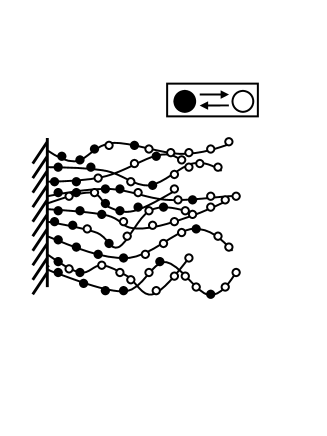
Figure 1: Schematic picture of a brush of a ”two-state polymer”. Open and filled circles depict monomers in the different, interconverting, monomeric states.

This approach is of interest because of a number of reasons: (i) $\chi_{eff}(T,\phi)$ determines a number of important characteristics of the brush among them the concentration profile, the distribution of free-ends and the force profile associated with the compression of the brush. Thus, a description of the brush behavior in terms of $\chi_{eff}(T,\phi)$ accounts for the leading brush properties and facilitates the comparison of the predictions of the different models. The specific features of the individual models and their parameters come into play when the distribution of the monomer states is of interest. However, as we shall discuss, even in this case it is convenient to first specify the brush characteristics in terms of $\chi_{eff}(T,\phi)$. (ii) The formulation of the theory in terms of $\chi_{eff}(T,\phi)$ underlines the relationship to the measurable

$$\overline{\chi}(T,\phi)=\chi_{eff}-(1-\phi)\partial\chi_{eff}/\partial\phi$$

as obtained from the study of the colligative properties of the polymer solutions.Flory ; wolfBook ; Flory1 ; rev $\overline{\chi}(T,\phi)$ is helpful in determining the parameters of the models. In the context of brushes, the behavior of $\overline{\chi}(T,\phi)$ provides, as we shall discuss, a useful diagnostic for systems expected to exhibit a vertical phase separation within the brush. (iii) While our discussion focuses on the two-state models cited above, the analysis can be extended to other modelssanchez ; Freed that yield a $\phi$ dependent $\chi_{eff}$. (iv) The SCF theory of brushes characterized by $\chi_{eff}(T,\phi)$ suggests useful tests for the occurrence of vertical phase separation. This is of interest, as we shall discuss in the final section, because of experimental indications that such behavior occurs in brushes of PNIPAM. (v) The concentration profiles obtained from the SCF theory are essentially identical to those derivedBH2 from the Pincus approximation where the distribution of free-ends is assumed rather than derived.Pincus ; Pincus1 In marked contrast, the compression force profiles are sensitive to the distribution of free-ends and the two methods yield different results.

The two-state models differ in their identification of the interconverting states. Within the $n$-cluster modeln-Cluster1 ; n-Cluster2 one is a bare monomer while the second is a monomer incorporated into a stable cluster of $n$ monomers. In the remaining models one of the monomeric states is hydrophilic and the other is hydrophobic. The hydrophilic state is preferred at low $T$ while the hydrophobic state is favored at high $T$. In the Karlstrom modelKarlstrom the two states differ in their dipole moment and their interconversion involves an internal rotation. The models of Matsuyama and Tanaka,Matsuyama Bekiranov et alBekiranov and of DormindotovaDormidPhase assume that the hydrophilic monomeric state forms a H-bond to a water molecule while the hydrophobic state does not. The brush structure within the Karlstrom model was studied using numerical SCF theory of the Scheutjens-Fleer typeLinse ; Bjorling and allowed to rationalize the aggregation behavior of copolymers incorporating PEO blocks.Linse1 The brush structure within the $n$-cluster model was studied using SCF theoryWagner and by simulations.Mattice These reveal the possibility of a vertical phase separation within the brush giving rise to a discontinuity in the concentration profile. In turn, this was invoked in order to rationalize observations about the collapse of PNIPAM brushes.Napper The force profiles due to the compression of brushes described by the $n$-cluster model were also analyzed.AHcluster ; Sevick The studies of brushes of ”two-state polymers” focused on a particular model and were formulated in terms of the corresponding free energy. This obscured common features between the different models and hampered the comparison between them. For example, while a vertical phase separation is possible within all two-state models, this scenario was mainly studied for the $n$-cluster model thus creating a misleading impression about the physical origins of this phenomenon.

Our discussion concerns a brush of flexible ”two-state” chains, terminally grafted to a planar surface. We assume that the chains are monodisperse and that each chain incorporates $N$ monomers. The surface area per chain, $\sigma$, is constant and the surface is assumed to be non-adsorbing for the two monomeric states. The free energy per lattice site is

$$f_{\infty}(\phi,T)/kT=(1-\phi)\ln(1-\phi)+\chi_{eff}(\phi,T)\phi(1-\phi)$$ (1)

This form corresponds to the $N\rightarrow\infty$ limit. It is appropriate for brushes of any $N$ because the grafted chains lose their mobility and thus have no translational entropy. The application of our analysis to a particular case is illustrated for the Karlstrom model. However, most of our analysis is model independent in that $\chi_{eff}(T,\phi)$ is not specified explicitly. The only assumption made is that $\overline{\chi}(T,\phi)$ can be expanded in powers of $\phi$

$$\overline{\chi}(T,\phi)=\sum_{i=0}\overline{\chi}_{i}(T)\phi^{i}$$

where the $\overline{\chi}_{i}(T)$ are specific to a given model. For simplicity we further limit the discussion to systems where the first three terms provide an accurate description of $\overline{\chi}(T,\phi)$. As we shall discuss, the presence of a third order term is the minimal condition for the possibility of a vertical phase separation within the brush. The power series expansion of $\overline{\chi}(T,\phi)$ is clearly related to the virial expansion of the osmotic pressure, $\pi$. The two differ in that the second incorporates terms originating in the translational entropy. In discussions of the SCF theory $f_{\infty}(\phi)/kT$ was often approximated by the second and third terms in the virial expansion of the Flory-Huggins free energy. From this point of view it is important to note two points: (i) in the power series of $\overline{\chi}(T,\phi)$ all the coefficients are $T$ dependent and can change sign. (ii) Use of $\overline{\chi}(T,\phi)$ series expansion including a $\phi^{3}$ term corresponds to a virial expansion incorporating a $\phi^{4}$ term.

The next five sections, II–VI, are devoted to the model independent aspects of the SCF theory based on $f_{\infty}(\phi,T)/kT$ with $\phi$ dependent $\chi_{eff}$. In section II we formulate the analytical SCF model for $\chi_{eff}(\phi,T)$ as a generalization of the familiar SCF theory of brushes.Semenov ; Milner ; MilnerBrush ; Skvortsov ; Zhulina The concentration profiles and their moments are discussed in section III. The technical details corresponding to section III are described in Appendix A. Section IV discusses the distribution of free ends while the technical details are given in Appendix B. The force profiles associated with the compression of the brush are analyzed in section V. In every case we distinguish between brushes characterized by a continuos concentration profile and those exhibiting a vertical phase separation. Finally, in section VI we illustrate the implementation of our analysis to the Karlstrom model. In particular, we obtain the corresponding $\chi_{eff}(T,\phi)$, $\overline{\chi}(T,\phi)$ and the distribution of monomeric states in the brush.

II The SCF theory for $\chi_{eff}(T,\phi)$

Consider a brush of neutral and flexible polymers comprising $N$ monomers of size $a$. Each chain is grafted by one end onto an impermeable, non-adsorbing, planar surface. The area per chain is denoted by $\sigma$ and $H$ is the maximal height of the brush. Following refs. Skvortsov, ; Zhulina, , the free energy per chain, $F_{chain}$, consists of two terms: an interaction free energy, $F_{int}$, and an elastic free energy, $F_{el}$, $F_{chain}=F_{int}+$ $F_{el}$. The interaction free energy per chain is

$$\frac{F_{int}}{kT}=\frac{\sigma}{a^{3}}\int_{0}^{H}f_{\infty}(\phi)dz$$ (2)

where the interaction free energy density $f_{\infty}(\phi)$ is given by (1). In a strong stretching limit, when the chains are extended significantly with respect to Gaussian dimensions, the elastic free energy is²⁷

$$\frac{F_{el}}{kT}=\frac{3}{2a^{2}}\int_{0}^{H}g(z^{\prime})dz^{\prime}\int_{0}^{z^{\prime}}E(z,z^{\prime})dz.$$ (3)

Here $E(z,z^{\prime})=dz/dn$ characterizes the local chain stretching at height $z$ when the free end is at height $z^{\prime}$. $g(z^{\prime})$ specifies the height distribution of the free ends and obeys the normalization condition $\int_{0}^{H}g(z^{\prime})dz^{\prime}=1$.

The concentration of monomers, $\phi(z)$, at height $z$ is specified by

$$\phi(z)=\frac{a^{3}}{\sigma}\int_{z}^{H}\frac{g(z^{\prime})dz^{\prime}}{E(z,z^{\prime})}$$ (4)

Since each chain consists of $N$ monomers we have

$$N=\frac{\sigma}{a^{3}}\int_{0}^{H}\phi(z)dz$$ (5)

At the same time

$$N=\int_{0}^{z^{\prime}}\frac{dz}{E(z,z^{\prime})}$$ (6)

which can be regarded as a normalization condition for the function $E(z,z^{\prime})$.

The equilibrium $\phi(z)$ in the brush is determined by the variation of the functional $F_{chain}$ with respect to $E(z,z^{\prime})$ and $g(z^{\prime})$ subject to the constraints (5) and (6) yielding

$$E(z,z^{\prime})=\frac{\pi}{2N}\sqrt{z^{\prime 2}-z^{2}}$$ (7)

and

$$\mu(\phi)=\lambda-Bz^{2}$$ (8)

where $B=3\pi^{2}/8N^{2}a^{2}$, $\lambda$ is the Lagrange multiplier associated with constraint (5) and $\mu(\phi)=\partial f_{\infty}(\phi)/\partial\phi$ is the exchange chemical potential. Up to this point the SCF theory is identical to the familiar versions, as obtained for $\chi=\chi(T)$.

For dilute brushes, $\sigma>>1,$ immersed in a good solvent and when $\chi$ is independent of$\phi$, $\chi_{eff}(\phi,T)=\chi(T)\ll 1/2$, the chemical potential is linear in $\phi$, $\mu(\phi)\sim\phi$ . In this case, when binary interactions are dominant, eq. (8) leads to a parabolic concentration profile.MilnerBrush ; Zhulina At higher grafting densities, $\sigma\geq 1,$ higher order terms become significant. These were typically handled by incorporation of the third virial term.MilnerBrush ; Zhulina However, as discussed in the introduction, deviations from these scenarios are expected when $\chi_{eff}(\phi)$ varies with $\phi$ and $\mu(\phi)$, as obtained from (1), assumes the form

$$\mu(\phi) = -\ln\left(1-\phi\right)-1+\chi_{eff}(\phi)-2\chi_{eff}(\phi)\phi+$$ (9)

$$\phi(1-\phi)\frac{\partial\chi_{eff}(\phi)}{\partial\phi}$$

Since colligative measurements yield $\overline{\chi}(\phi)=\chi_{eff}(\phi)-(1-\phi)\partial\chi_{eff}(\phi)/\partial\phi$foot2 rather than $\chi_{eff}(\phi)$ it useful to express $\mu(\phi)$ as

$$\mu(\phi)=-\ln(1-\phi)-1+\chi_{eff}(0)-\int_{0}^{\phi}\overline{\chi}(\phi)d\phi-\phi\overline{\chi}(\phi)$$ (10)

Finally, the Lagrange multiplier $\lambda$ is determined by the concentration at the outer edge of the brush, $\phi_{H}\equiv\phi(z=H)$

$$\lambda = BH^{2}+\mu(z=H)$$ (11)

$$= BH^{2}-\ln(1-\phi_{H})-1+\chi_{eff}(0)-$$

$$\int_{0}^{\phi_{H}}\overline{\chi}(\phi)d\phi-\phi_{H}\overline{\chi}(\phi_{H}),$$

In turn, $\phi_{H}$ of a free brush is set by the osmotic pressure at $H$ that is, $\pi_{osm}(\phi_{H})=\left.\phi^{2}\partial\left[f_{\infty}(\phi)/\phi\right]/\partial\phi\right|_{\phi=\phi_{H}}=0$, leading to

$$-\ln(1-\phi_{H})-\phi_{H}-\overline{\chi}(\phi_{H})\phi_{H}^{2}=0$$ (12)

In a good solvent $\phi_{H}=0$.

III The Concentration Profiles and Their Moments

In order to obtain $\phi(z)$ it helpful to express (8) as

$$\Delta\mu(\phi)=B(H^{2}-z^{2})$$ (13)

where

$$\Delta\mu(\phi)=-\ln\frac{1-\phi}{1-\phi_{H}}-\int_{\phi_{H}}^{\phi}\overline{\chi}(\phi)d\phi+\phi_{H}\overline{\chi}(\phi_{H})-\phi\overline{\chi}(\phi)$$ (14)

Equation (13) does not specify $\phi(z)$ directly. Rather, it yields $z(\phi)=\sqrt{H^{2}-\Delta\mu(\phi)/B}$. The brush height is determined in terms of the monomer volume fraction at the surface, $\phi_{0}=\phi(z=0)$, leading to $H=\sqrt{\Delta\mu(\phi_{0})/B}$ and

$$z(\phi)=\sqrt{\frac{\Delta\mu(\phi_{0})-\Delta\mu(\phi)}{B}}$$ (15)

$\phi(z)$ is determined by equation (15) together with the normalization condition (5), which relates $\phi_{0}$ to the grafting density, $1/\sigma$.

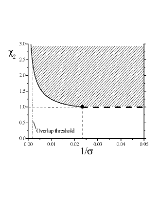
Figure 2: The state diagram of a brush with $\overline{\chi}(\phi)=1/2+\chi_{2}\phi^{2}$ and $N=200$ in the $\chi_{2}$, $1/\sigma$ plane. Vertical phase separation occurs in the hatched region. At $\bullet$ $\phi_{0}=\phi_{-}(T)$. The dashed line, at higher $1/\sigma$, corresponds to brushes exhibiting an inflection point at altitudes that increase with $1/\sigma$. The boundary for lower $1/\sigma$ corresponds to $\phi_{-}$ $\phi_{+}$ coexistence at the grafting surface.

We now distinguish between two cases. In one the concentration profile is continuous while in the second a discontinuity occurs due to vertical phase separation. In the first case (5) may be expressed as

$$N=\frac{\sigma}{a^{3}}\int_{\phi_{0}}^{\phi_{H}}\phi\frac{\partial z}{\partial\phi}d\phi$$ (16)

The concentration profile for a given $\sigma$ is fully specified by (15) and (16). A vertical phase separation in the brush results in a discontinuity at height $H_{t}$. At this altitude two phases coexist: a dense inner phase with a monomer volume fraction $\phi_{+}(H_{t})$ and a dilute outer phase with $\phi_{-}(H_{t})$. In this case the normalization condition (5) assumes the form

$$N=\frac{\sigma}{a^{3}}\int_{\phi_{0}}^{\phi_{+}(H_{t})}\phi\frac{\partial z}{\partial\phi}d\phi+\frac{\sigma}{a^{3}}\int_{\phi_{-}(H_{t})}^{\phi_{H}}\phi\frac{\partial z}{\partial\phi}d\phi$$ (17)

where $\phi_{+}(H_{t})$ and $\phi_{-}(H_{t})$ are determined by $\mu(\phi_{+})=\mu(\phi_{-})$ and $\pi(\phi_{+})=\pi(\phi_{-})$. $\phi(z)$ is now determined by equation (15) together with the normalization condition (17),

It is of interest to consider the phase behavior when $\overline{\chi}(\phi)$ is described by $\overline{\chi}(\phi)=\chi_{0}+\chi_{1}\phi+\chi_{2}\phi^{2}$. In the case of $\overline{\chi}(\phi)=\chi_{0}$ or $\overline{\chi}(\phi)=\chi_{0}+\chi_{1}\phi$ the critical point, as specified by $\partial^{2}f_{\infty}(\phi)/\partial\phi^{2}=\partial^{3}f_{\infty}(\phi)/\partial\phi^{3}=0$

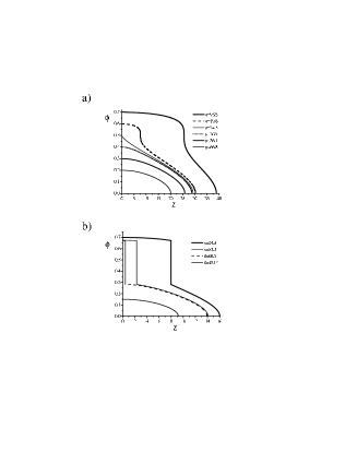
Figure 3: $\phi(z)$ for different areas per chain $\sigma$ when $\overline{\chi}(\phi)=1/2+\chi_{2}\phi^{2}$. (a) $\chi_{2}=1$ (b) $\chi_{2}=1.05$. In every case $N=200$.FootFig

$$\frac{1}{1-\phi}-2\overline{\chi}(\phi)-\phi\frac{\partial\overline{\chi}(\phi)}{\partial\phi} = 0$$ (18)

$$\frac{1}{\left(1-\phi\right)^{2}}-3\frac{\partial\overline{\chi}(\phi)}{\partial\phi}-\phi\frac{\partial^{2}\overline{\chi}(\phi)}{\partial\phi^{2}} = 0$$ (19)

occurs at $\phi_{c}=0$. This corresponds to the familiar case of a polymer rich phase in coexistence with a neat solvent. In this situation there is no vertical phase separation within the brush and the concentration profile is continuous. A second type of phase separation,n-Cluster1 ; n-Cluster2 ; Solc1 ; Solc2 associated with a discontinuous $\phi(z)$, is possible when higher order terms are involved. For $\overline{\chi}(\phi)=1/2+\chi_{2}\phi^{2}$ a critical point occurs at $\phi_{c}=1/2$ and $\chi_{2c}=1$. In the vicinity of the critical point, for $\chi_{2}\gtrsim 1$ and $\phi\gtrsim$ $1/2$ the coexistence curve is well approximated by the spinodal line $\partial^{2}f_{\infty}(\phi)/\partial\phi^{2}=0$

$$\frac{1}{1-\phi}-1-4\chi_{2}\phi^{2}=0$$ (20)

leading to $\phi_{\pm}=\frac{1}{2}\pm\frac{1}{2}\sqrt{1-1/\chi_{2}}$. The state diagram of a brush in the $\chi_{2},1/\sigma$ plane when eq. (20) applies is shown in Fig. 2. Concentration profiles obtained from $\overline{\chi}(\phi)$ of this form are depicted in Fig. 3.

Figure 4: Plots of $\phi(z)$ (a) and $g(z)$ (b) above and below the critical point for $\overline{\chi}(\phi)=1/2+\chi_{2}\phi^{2}$, $\sigma=17$ and $N=200$. In all cases, the outer phase is swollen.FootFig

Experimentally, the brush thickness $H$ is inaccessible. Certain experimental technique yield $\phi(z)$ allowing one to obtain moments of $\phi(z)$

$$\langle z\rangle=\frac{\int_{0}^{H}z\phi(z)dz}{\int_{0}^{H}\phi(z)dz}=\frac{\sigma}{Na^{3}}\int_{0}^{H}z\phi(z)dz$$ (21)

$$\langle z^{2}\rangle=\frac{\int_{0}^{H}z^{2}\phi(z)dz}{\int_{0}^{H}\phi(z)dz}=\frac{\sigma}{Na^{3}}\int_{0}^{H}z^{2}\phi(z)dz.$$ (22)

Other techniques, such as ellipsometry, measure $\langle z\rangle$.charmet As we shall discuss, the $\sigma$ dependence of the moments provides useful information on the brush structure. The details of the calculation of these moments are described in Appendix A.

When $\phi(z)$ is continuous, both moments increase smoothly with the grafting density. In marked contrast, vertical phase separation within the brush gives rise to a non-monotonic behavior. In particular, both $\langle z\rangle$ and $\sqrt{\langle z^{2}\rangle}$ exhibit a minimum at intermediate $\sigma$. A vertical phase separation gives rise to a plateau in the $H$ vs. $\sigma$ plot (Fig. 8) while in the plots of $\langle z\rangle$ and $\sqrt{\langle z^{2}\rangle}$ vs. $\sigma$ it is associated with a minimum (Fig. 6 and Fig. 7). The physical origin of this behavior is the partitioning of the monomers between the inner dense phase and the outer dilute one. The minima are traceable to the higher weight give to the inner phase. Since the inner phase is denser, the onset of vertical phase separation is associated with a decrease $\langle z\rangle$ and $\sqrt{\langle z^{2}\rangle}$. These features provide a useful diagnostic for the occurrence of a vertical phase separation in the brush. The SCF analysis in this section confirms earlier resultsBH2 obtained by utilizing the Pincus approximation.Pincus ; Pincus1 As we shall discuss this is the case for properties that are insensitive to the precise form of $g(z)$. In marked contrast, the compression force profile (section V) does depend on $g(z)$ and the SCF result differ from the one obtained from the Pincus approximation.

Figure 5: Plots of $\phi(z)$ (a) and $g(z)$ (b) for the case of two coexisting dense phases with $\overline{\chi}(\phi)=0.51+\chi_{2}\phi^{2}$, $\sigma=18$ and $N=200$.FootFig

IV The Distribution of Free Ends

The SCF formalism allows to obtain the height distribution of free ends, $g(z)$. Current experimental techniques do not allow to probe $g(z)$ directly. However, $g(z)$ is of interest because it plays a role in the calculation of the compression force profile. When $\chi=const$ the brush structure is dominated by the contributions of the second and third virial terms of $F_{int}$. Three scenarios emerge. In a good solvent the ends are distributed throughout the brush and $g(z)$ is a smooth function vanishing at $z=0$ and $z=H$. When the brush is collapsed in a poor solvent the ends reside preferentially at the outer edge of the brush and $g(z)$ diverges at $H$. In a $\theta$ solvent $g(z)$ increases smoothly with $z$ but does not diverge.Skvortsov ; Zhulina As we shall see, a new scenario emerges when a vertical phase separation occurs. In particular, $g(z)$ will then diverge at the phase boundary indicating localization of the ends at the boundary. We will obtain $g(z)$ from the integral equation (4). The details of the calculation are described in Appendix B.

Figure 6: $\langle z\rangle$ as a function of $\sigma$ for different $\chi_{2}$ values and $N=300$.FootFig

$g(z)$ of a brush with a continuous profile (Fig. 4a) is specified by

$$g(z) = z\frac{\sigma}{Na^{3}}\left(\frac{\phi_{H}}{\sqrt{H^{2}-z^{2}}}+\right.$$ (23)

$$\left.\sqrt{B}\int_{\phi_{H}}^{\phi}\frac{d\phi^{\prime}}{\sqrt{\Delta\mu(\phi)-\Delta\mu(\phi^{\prime})}}\right)$$

where $\phi$ and $z$ are related by (13). When a vertical separation occurs within the brush, equation (4) yields now two expressions, for $\phi(z)$. At the outer edge, $H_{t}<z<H$

$$\phi(z)=\frac{a^{3}}{\sigma}\int_{z}^{H}\frac{g(z^{\prime})dz^{\prime}}{E(z,z^{\prime})}$$ (24)

while at the inner dense phase, $0<z<H_{t}$

$$\phi(z)=\frac{a^{3}}{\sigma}\int_{z}^{H_{t}}\frac{g(z^{\prime})dz^{\prime}}{E(z,z^{\prime})}+\frac{a^{3}}{\sigma}\int_{H_{t}}^{H}\frac{g(z^{\prime})dz^{\prime}}{E(z,z^{\prime})}$$ (25)

In the outer region only free ends with $H_{t}<z$ contribute while for the inner phase all free ends are involved.

The expression for $g(z)$ in the two regions are given below while the details of the derivation are presented in appendix B. At the outer phase, $H_{t}<z<H$

$$g(z) = z\frac{\sigma}{Na^{3}}\left(\frac{\phi_{H}}{\sqrt{H^{2}-z^{2}}}+\right.$$ (26)

$$\left.\sqrt{B}\int_{\phi_{H}}^{\phi}\frac{d\phi^{\prime}}{\sqrt{\Delta\mu(\phi)-\Delta\mu(\phi^{\prime})}}\right)$$

while in the inner phase, $0<z<H_{t}$

$$g(z)=\frac{z\sigma}{Na^{3}}\left[\frac{\phi_{+}(H_{t})-\phi_{-}(H_{t})}{\sqrt{H_{t}^{2}-z^{2}}}+\frac{\phi_{H}}{\sqrt{H^{2}-z^{2}}}+\right.$$

$$\sqrt{B}\int_{\phi_{+}(H_{t})}^{\phi}\frac{d\phi^{\prime}}{\sqrt{\Delta\mu(\phi)-\Delta\mu(\phi^{\prime})}}+\frac{\sqrt{B}}{\pi}\sqrt{H_{t}^{2}-z^{2}}\times$$

$$\int_{\phi_{H}}^{\phi_{\_}(H_{t})}\frac{\frac{d\Delta\mu(\phi^{\prime})}{d\phi^{\prime}}d\phi^{\prime}}{\left(H^{2}-z^{2}-\frac{\Delta\mu(\phi^{\prime})}{B}\right)\sqrt{H^{2}-H_{t}^{2}-\frac{\Delta\mu(\phi^{\prime})}{B}}}\times$$

$$\left.\int_{\phi_{H}}^{\phi^{\prime}}\frac{d\phi^{\prime\prime}}{\sqrt{\Delta\mu(\phi^{\prime})-\Delta\mu(\phi^{\prime\prime})}}\right].$$ (27)

The first integral allows for the contribution of the inner phase and the second for the contribution of the outer phase. $g(z)$ (27) at the interval $0<z<H_{t}$ diverges at the phase boundary $z=H_{t}$. $g(z)$ (26) at the interval $H_{t}<z<H$ diverges at $H$ when the outer phase is collapsed and $\phi_{H}>0$. In this case the two coexisting phases are dense (Fig. 5). When $\phi_{H}=0$ the outer phase is swollen and $g(z)$ does not diverge at $H$ (Fig. 4b). A rough approximation yielding closed form expressions for $g(z)$ for discontinuous brushes is described in Appendix C.

Figure 7: $\sqrt{\langle z^{2}\rangle}$ as a function of $\sigma$ for different $\chi_{2}$ values and $N=300$.FootFig

V The Compression Force Profile of a ”Two-State” Brush

The surface force apparatus allows to measure the restoring force arising upon compression of a brush. For brushes of polymers characterized by a constant $\chi$ the force increases smoothly with the compression and the force profile is essentially featureless. When the brush consists of polymers characterized by $\overline{\chi}(\phi)$ the compression can induce a vertical phase separation even if the concentration profile of the brush is initially continuous. The existence of vertical phase separation, be it compression induced or not, gives rise to distinctive regimes in the force profile. In particular, the slope of the force vs. distance curve in different compression regimes can be markedly different. In such experiments $H$ is determined by the compressing surface rather than by $\sigma$. Accordingly, $\phi_{H}$ is set by the normalization condition (5) and not by $\pi(\phi_{H})=0$. The compression increases $F_{chain}$ and the restoring force per area $\sigma$ is

$$f(H)=-\frac{\partial F_{chain}}{\partial H}$$ (28)

In the following we obtain this force law for the case of compression by impenetrable, non-adsorbing surface.

Figure 8: $H$ as a function of $\sigma$ for different $\chi_{2}$ values and $N=300$.FootFig

For a brush with a continuous $\phi(z)$

$$\frac{F_{chain}}{kT}=\int_{\phi_{0}}^{\phi_{H}}\left[\frac{\sigma}{a^{3}}f_{\infty}(\phi)+\frac{3}{2a^{2}}\frac{\pi^{2}}{8N}z^{2}(\phi)g(\phi)\right]\frac{\partial z}{\partial\phi}d\phi$$ (29)

obtained by invoking $\int_{0}^{z^{\prime}}E(z^{\prime},z)dz=z^{\prime 2}\pi^{2}/(8N)$. Here $g(z)$ is given by (23), while $z(\phi)$ and $\partial z/\partial\phi$ are specified by (15). $f(H)$ is calculated numerically subject to the constraint (16). When the concentration at the wall, $\phi_{0}$, exceeds $\phi_{-}$, the brush undergoes a vertical phase separation and $\phi(z)$ is no longer continuous. In this case $F_{chain}$ assumes the form

Figure 9: The compression force profile for a brush with $\overline{\chi}(\phi)=1/2+1.05\phi^{2}$, $\sigma=120$ and $N=300$. The uncompressed brush is in a single phase state ($\phi_{0}<\phi_{-})$.FootFig

$$\frac{F_{chain}}{kT} = \frac{\sigma}{a^{3}}\int_{\phi_{0}}^{\phi_{H}}f_{\infty}(\phi)\frac{\partial z}{\partial\phi}d\phi+$$ (30)

$$\frac{3}{2a^{2}}\frac{\pi^{2}}{8N}\left[\int_{\phi_{0}}^{\phi_{+}(H_{t})}z^{2}(\phi)g(\phi)\frac{\partial z}{\partial\phi}d\phi+\right.$$

$$\left.\int_{\phi_{-}(H_{t})}^{\phi_{H}}z^{2}(\phi)g(\phi)\frac{\partial z}{\partial\phi}d\phi\right]$$

where $g(\phi)$ is specified by eqs. (27) for the inner phase and by (26) for the outer one. The conservation of monomers is enforced by the constraint (17).

Figure 10: $\phi(z)$ plots corresponding to the three regimes in Fig. 9. (a) single phase swollen phase, $H=12.9$, (b) a coexistence of a dense and a dilute phase, $H=6.1$, (c) single dense phase, $H=3.7$. In every case $\sigma=120$ and $N=300$.FootFig

When the conditions permit a vertical phase separation within the brush, it can take place in two ways. It can occur when the grafting density exceeds a certain critical value thus causing $\phi_{0}>\phi_{-}$. Alternatively, it can also take place as a result of compression when the grafting density does not lead to phase separation in the unperturbed brush. The development of $\phi(z)$ and $f(H)$ for this second case is depicted in figures 9 and 10 respectively. Initially, the brush retains the single phase structure and the associated force law. When the compression enforces $\phi_{0}>\phi_{-}$, a vertical phase separation occurs and is signalled by a weaker slope of the $f(H)$ vs. $H$ curve. Stronger compression causes complete conversion to a dense phase thus causing an abrupt increase in $f(H)$.

VI The Karlstrom Model and the distribution of monomeric states

Thus far, our discussion concerned brushes characterized by an arbitrary $\chi_{eff}(\phi)$. We now illustrate these considerations for the case of the Karlstrom model.Karlstrom We focus on this model because of its simplicity and its semiquantiative agreement with the phase diagram of aqueous solutions of PEO at atmospheric pressureKarlstrom and the measured $\overline{\chi}(T,\phi)$.BH Within this model the monomers exist in two states: a polar, hydrophilic state (A) and an apolar, hydrophobic state (B). The two intercovert via internal rotations. In the $N\rightarrow\infty$ limit the corresponding Flory-type free energy is

$$\frac{f_{\infty}(\phi)}{kT} = (1-\phi)\ln(1-\phi)+$$ (31)

$$\phi[p\ln p+(1-p)\ln(1-p)]+$$

$$\phi p\Delta\epsilon+\phi(1-\phi)[p\chi_{AS}+(1-p)\chi_{BS}]+$$

$$\phi^{2}\chi_{AB}p(1-p)$$

where $p$ denotes the fraction of monomers in the A state. The first term allows for the mixing entropy of the solvent while the second reflects the mixing entropy of the A and B states along the chain. $\Delta\epsilon$ is the energy difference between two states and $\phi p\Delta\epsilon$ allows for the effect of interconversion between them. The fourth term is the generalization of the $\chi\phi(1-\phi)$ in the Flory free energy to allow for the interactions of the two states with the solvent S. The interactions between $A$ and $B$ states gives rise to the last term.

The equilibrium value of $p$ for a given $\phi$ is specified by $\partial f_{\infty}/\partial p=0$ leading to

$$\frac{p}{1-p} = \exp\left[-\Delta\epsilon-(1-\phi)(\chi_{AS}-\chi_{BS})-\right.$$ (32)

$$\left.\phi\chi_{AB}(1-2p)\right]$$

The parameters used by KarlstromKarlstrom to fit phase diagram of PEO in water are $\chi_{As}=80.0/T$, $\chi_{Bs}=684.5/T$, $\chi_{AB}=155.6/T$, $\Delta\varepsilon=-625.2/T+\ln 8$. In the remainder of this section we consider brushes at $T=60^{o}$ C. The equilibrium $\chi_{eff}(\phi)$ is obtained by equating (31) and (32)

$$\chi_{eff}(\phi) = p\chi_{AS}+(1-p)\chi_{BS}+$$ (33)

$$\frac{\phi}{1-\phi}\left[\chi_{AB}p(1-p)+p\Delta\epsilon\right]+$$

$$\frac{p\ln p+(1-p)\ln(1-p)}{1-\phi}$$

where $p(\phi)$ is specified by (32). $\ \overline{\chi}=-\frac{\partial}{\partial\phi}\frac{f_{\infty}(\phi)}{\phi}$ together with (32) yield the equilibrium value

$$\overline{\chi}(\phi)=p\chi_{AS}+(1-p)\chi_{BS}-\chi_{AB}p(1-p)$$ (34)

Both $\chi_{eff}(\phi)$ and $\overline{\chi}(\phi)$ can be expanded in powers of $\phi$. The coefficients in the expansion depend on the parameters, $\Delta\epsilon$, $\chi_{AS}$, $\chi_{BS}$, $\chi_{AB}$. High order terms are of negligible importance and $\overline{\chi}(\phi)\approx 0.48+0.31\phi+0.07\phi^{2}$ provides a good approximation for $\overline{\chi}(\phi)$.

Figure 11: A plot of the fraction of hydrophilic states, $p$, vs. $z$, in the Karlstrom modelKarlstrom for different $\sigma$. In every case $\chi_{As}=80.0/T$, $\chi_{Bs}=684.5/T$, $\chi_{AB}=155.6/T$, $\Delta\varepsilon=-625.2/T+\ln 8$, $N=300$ $T=60^{o}$ C. FootFig

Equation (32) allows to relate the volume fraction $\phi$ to $p$, the fraction of hydrophilic A states, as

$$\phi(p)=\frac{\ln\frac{p}{1-p}+\Delta\epsilon+\chi_{AS}-\chi_{BS}}{\chi_{AS}-\chi_{BS}-\chi_{AB}(1-2p)}$$ (35)

Accordingly, the exchange chemical potential can be specified in terms of $p$, i.e. $\Delta\mu(\phi(p))$. In turn, eq. (13) enables us to obtain $z=z(p)$. To this end we invoke two boundary conditions: (i) In this range of parameters the brush is swollen and $\phi$ vanishes at the outer edge, $\phi_{H}=\phi(p=p_{H})=0$ where $p_{H}$ is the value of $p$ at the height $H$. (ii) At the grafting surface we have $\Delta\mu(z=0,p=p_{0})=BH^{2}$, where $p_{0}$ is the value of $p$ at $z=0$. In addition we utilize the conservation of monomers as given by (16). The corresponding plots of $p=p(z)$ as well as the concentration profiles of the two states are depicted, for different $\sigma$, in Fig. 11 and in Fig. 12. Since all brushes considered are swollen, with $\phi_{H}=0$, the $p$ values at the outer edge of the brush, $z=H$ are identical, $p=p_{H}$. Increasing grafting density leads to higher concentration at the grafting surface. This favors the hydrophobic B state and lower $p$ at the surface. For the chosen parameters, the minimal value of $p$, corresponding to a PEO melt ($\phi=1$), is $p_{\ast}=0.45$.

Figure 12: The overall $\phi(z)$ and the corresponding concentration profiles of the monomeric states $\phi_{A}(z)=p(z)\phi(z)$ and $\phi_{B}(z)=[1-p(z)]\phi(z)$ within the Karlstrom model for the conditions specified in Fig. 11.FootFig

VII Discussion

In this article we presented a common framework for the analysis of the structure of brushes of neutral water-soluble polymers (NWSP) that own their solubility to the formation of H-bonds with water molecules. Our analysis concerned a family of two-state models developed for PEO but applicable, in principle, to other NWSP. The particular aspects of the models were grouped into $\chi_{eff}(T,\phi)$ thus allowing for a unified discussion of the brush structure within these models. Significant part of the discussion concerned brushes exhibiting vertical phase separation that can occur for polymers capable of a second type of phase separation. In particular, we examined the distinctive behavior of plots of $\langle z\rangle$ and $\sqrt{\langle z^{2}\rangle}$ vs. $\sigma$ and the compression force profiles associated with such brushes. $\phi(z)$ and its moments are insensitive to the precise form of $g(z)$ and the SCF analysis recovers the results obtained earlierBH2 by the use of the Pincus approximation.Pincus ; Pincus1 In marked contrast, the compression force law does depend on $g(z)$ and a full SCF analysis is necessary in order to obtain the correct results. These features are useful criteria for the occurrence of vertical phase separation. Such criteria are of interest because of indirect experimental indications that brushes of PNIPAM exhibit this effect. Among these indications the following are especially noteworthy. First, is an early study by Zhu and NapperNapper of the collapse of PNIPAM brushes grafted to latex particles immersed in water. This revealed a collapse involving two stages. An “early collapse”, took place below $30^{o}$ C, at “better than $\theta$-conditions”, and did not result in flocculation of the neutral particles. Upon raising the temperature to “worse than $\theta$-conditions” the collapse induced flocculation. This indicates that the colloidal stabilization imparted by the PNIPAM brushes survives the early collapse. It lead to the interpretation of the effect in terms of a vertical phase separation within the brush associated with a second type of phase separation as predicted by the $n$-cluster model. More recently, Balamurugan et alBalamurugan used Surface Plasmon Resonance (SPR) and contact angle measurements with water to characterize PNIPAM brushes ”grafted from” a self-assembled monolayer on gold. The brush properties were studied at between $10^{o}$ C and $40^{o}$ C. The SPR measurements indicated gradual variation of the brush properties. In marked contrast, the contact angle measurements revealed an abrupt change at $\sim 32^{o}$ C. Both experiments are consistent with a brush undergoing vertical phase separation such that the outer phase is hydrophilic. Within this picture, the abrupt changes reported in the wetting and aggregation behavior correspond than to the onset of a single, dense and hydrophobic phase. This picture is also supported by recent study of the phase behavior of PNIPAM by Afroze et al.A Early study of the phase behavior of PNIPAM in water, by Heskins and Guillet,HG identified a LCST at $\phi_{c}\simeq 0.16$ and $T_{c}\simeq 31.0^{o}$ C. In marked contrast, the work of Afroze et alA identified PNIPAM as a polymer undergoing a second type of phase separation. In particular: (i) While the LCST of PNIPAM depends on $N$ the LCST occurs around $T_{c}\simeq 27-28^{o}$ C and $\phi_{c}\simeq 0.43$ (ii) In the limit of $\phi\rightarrow 0$, the phase separation occurs, depending on $N$, between $30^{o}$ C and $34^{o}$ C. Thus, the phase diagram of Afroze et al suggests that a vertical phase separation is indeed expected in brushes of PNIPAM.BH2 Systematic Neutron Reflectometry (NR) studies of PNIPAM brushes will eventually provide clearer picture of the situation. Early studies were hampered by high polydispersity as well as difficulties in determining $N$ and $\sigma$.Yim With this in mind, the NR results revealed that the structure of PNIPAM brushes in acetone was very different from their structure in water, both at $20^{o}$ C and at $55^{o}$ C. In acetone the concentration profile was smoothly decaying while in water it consisted of a narrow, inner, dense region and an outer, extended and dilute region. More recent work utilized NR,Yim1 to study samples with lower polydispersity and higher grafting density between $20^{o}$ C and $40^{o}$ C. Importantly, the results indicate that most of the conformational change occurred between $28^{o}$ C and $34^{o}$ C though the corresponding concentration profiles were not reported. The results suggest a repartitioning of the monomers between a dilute outer tail and an inner dense region.Yim2 Finally, recent experimental results of Hu at alHurec are suggestive of the predictions obtained above concerning the variation of $\langle z\rangle$ upon decreasing $\sigma$ (Fig. 6). Hu et al studied the thickness of a PNIPAM brush grafted to spherical microgels of copolymers of PNIPAM and acrylic acid 2-hydroxyethyl ester (HEA). The microgels shrink as $T$ increases from $24^{o}$ C to $36^{o}$ C thus inducing a decrease in $\sigma$. Remarkably, the thickness of the brush initially decreases in the range $27^{o}$ C to $32^{o}$ C but subsequently increases upon further heating in the range $27^{o}$–$32^{o}$ C. Unfortunately, in this experiment it is impossible to separate the effects due to change in $T$ from those to the change in $\sigma$ because the $T$ is used to tune $\sigma$.

In confronting experimental results with theoretical predictions concerning the vertical phase separation it is important to note two points. First, polydispersity in $N$ and in $\sigma$ can smooth out the discontinuity in $\phi(z)$. These factors give rise to domains with different $\phi_{0}$. In turn, the altitude of the discontinuity in these domains will also differ. NR measurements will reflect the weighted average of these domains. Polydispersity in $N$ can lead to further strengthening of this effect if $\chi_{eff}$ depends on $N$. Second, the vertical phase separation involves a first order phase transition. Accordingly, nucleation dynamics may play a role and it is necessary to allow for the possibility of long relaxation times.

Appendix A Calculation of the average thickness

For a $\phi(z)$ (21) is evaluated using integration by parts utilizing $d\Delta\mu=-2Bzdz$:

$$\langle z\rangle = \frac{\sigma}{Na^{3}}\frac{1}{2B}\int_{0}^{BH^{2}}\phi(z)d\Delta\mu$$ (36)

$$= \frac{\sigma}{Na^{3}}\left(H^{2}\frac{\phi_{0}}{2}-\frac{1}{2B}\int_{\phi_{H}}^{\phi_{0}}\Delta\mu(\phi)d\phi\right)$$

For a discontinuous $\phi(z)$ (21) this procedure leads to

$$\langle z\rangle = \frac{\sigma}{Na^{3}}\left[\int_{0}^{H_{t}}z\phi(z)dz+\int_{H_{t}}^{H}z\phi(z)dz\right]$$ (37)

$$= \frac{\sigma}{Na^{3}}\frac{1}{2B}\left(\int_{B(H^{2}-H_{t}^{2})}^{BH^{2}}\phi(z)d\Delta\mu+\right.$$

$$\left.\int_{0}^{B(H^{2}-H_{t}^{2})}\phi(z)d\Delta\mu\right)$$

$$= \frac{\sigma}{Na^{3}}[H^{2}\frac{\phi_{0}}{2}-\left(H^{2}-H_{t}^{2}\right)\frac{\phi_{+}(H_{t})-\phi_{-}(H_{t})}{2}$$

$$- \frac{1}{2B}\int_{\phi_{+}(H_{t})}^{\phi_{0}}\Delta\mu(\phi)d\phi-\frac{1}{2B}\int_{\phi_{H}}^{\phi_{-}(H_{t})}\Delta\mu(\phi)d\phi]$$

The evaluation of (22) in the case of a continuous $\phi(z)$ involves introducing the variable $\Delta\mu=B(H^{2}-z^{2})$ and invoking $z=\sqrt{H^{2}-\Delta\mu/B}$. Integration by parts leads to

$$\langle z^{2}\rangle = \frac{\sigma}{Na^{3}}\frac{1}{2B}\int_{0}^{BH^{2}}z\phi(z)d\Delta\mu$$ (38)

$$= -\frac{\sigma}{Na^{3}}\frac{1}{2B}\int_{\Delta\mu=0}^{\Delta\mu=BH^{2}}\Delta\mu d(z\phi(z))$$

$$= -\frac{\sigma}{Na^{3}}\frac{1}{2B}\int_{\phi_{H}}^{\phi_{0}}\left(\phi\frac{\partial z}{\partial\phi}+z\right)\Delta\mu d\phi$$

Using

$$\frac{\partial z}{\partial\phi}=-\frac{1}{B\sqrt{H^{2}-\Delta\mu/B}}\frac{\partial\Delta\mu}{\partial\phi}$$ (39)

we obtain the final expression

$$\langle z^{2}\rangle = \frac{\sigma}{Na^{3}}\frac{1}{2B^{2}}\int_{0}^{\phi_{0}}\frac{\phi\Delta\mu\frac{\partial\Delta\mu}{\partial\phi}}{\sqrt{H^{2}-\Delta\mu/B}}d\phi-$$ (40)

$$\frac{1}{2B}\int_{0}^{\phi_{0}}\Delta\mu\sqrt{H^{2}-\Delta\mu/B}d\phi$$

where $\Delta\mu$ is specified by (14).

Following a similar procedure for a discontinuous $\phi(z)$ (22) yields

$$\langle z^{2}\rangle = \frac{\sigma}{Na^{3}}\left[\int_{0}^{H_{t}}z^{2}\phi(z)dz+\int_{H_{t}}^{H}z^{2}\phi(z)dz\right]$$ (41)

$$= \frac{\sigma}{Na^{3}}\frac{1}{2B}\left(\int_{B(H^{2}-H_{t}^{2})}^{BH^{2}}z\phi(z)d\Delta\mu+\right.$$

$$\left.\int_{0}^{B(H^{2}-H_{t}^{2})}z\phi(z)d\Delta\mu\right)$$

$$= \frac{\sigma}{Na^{3}}\left[\frac{1}{2B^{2}}\int_{\phi_{+}(H_{t})}^{\phi_{0}}\frac{\phi\Delta\mu\frac{\partial\Delta\mu}{\partial\phi}}{\sqrt{H^{2}-\Delta\mu/B}}d\phi-\right.$$

$$\frac{1}{2B}\int_{\phi_{+}(H_{t})}^{\phi_{0}}\Delta\mu\sqrt{H^{2}-\Delta\mu/B}d\phi$$

$$+\frac{1}{2B^{2}}\int_{0}^{\phi_{-}(H_{t})}\frac{\phi\Delta\mu\frac{\partial\Delta\mu}{\partial\phi}}{\sqrt{H^{2}-\Delta\mu/B}}d\phi-$$

$$\frac{1}{2B}\int_{0}^{\phi_{-}(H_{t})}\Delta\mu\sqrt{H^{2}-\Delta\mu/B}d\phi$$

$$\left.-H_{t}\left(H^{2}-H_{t}^{2}\right)\frac{\phi_{+}(H_{t})-\phi_{-}(H_{t})}{2}\right]$$

Appendix B Calculation of the distribution of ends function

Upon introducing the variables $\rho=H^{2}-z^{2}$, $t=H^{2}-z^{\prime 2}$ and $g(z^{\prime})dz^{\prime}=-f(t)dt$ eq. (4) assumes the form of an Abel integral equation

$$v(\rho)=\int_{0}^{\rho}\frac{f(t)dt}{\sqrt{\rho-t}},$$ (42)

where $v(\rho)=\frac{\pi\sigma}{2Na^{3}}\phi(z)$ whose solution (42) is

$$f(\rho)=\frac{1}{\pi}\left(\frac{v(0)}{\sqrt{\rho}}+\int_{0}^{\rho}\frac{1}{\sqrt{\rho-t}}\frac{dv(t)}{dt}dt\right).$$ (43)

It is convenient to rewrite the integral in (43) as

$$\int_{0}^{\rho}\frac{1}{\sqrt{\rho-t}}\frac{dv(t)}{dt}dt=\int_{v(H)}^{v(z)}\frac{dv}{\sqrt{\rho-t(v)}}$$ (44)

$$= \frac{\pi\sigma}{2Na^{3}}\sqrt{B}\int_{\phi_{H}}^{\phi}\frac{d\phi^{\prime}}{\sqrt{\Delta\mu(\phi)-\Delta\mu(\phi^{\prime})}}$$

where $\Delta\mu(\phi)$ is given by (13). Substituting this integral into (43) while noting that $v(0)=\frac{\pi\sigma}{2Na^{3}}\phi_{H}$ and $g(z)=2zf(\rho)$, leads to $g(z)$ in the form (23). This equation yields a simple form $z(\phi)$ rather than for $\phi(z)$. Thus, it is naturally to consider $g(z)$ as a parametric function

$$g(\phi) = \frac{\sigma}{Na^{3}}\sqrt{H^{2}-\Delta\mu(\phi)/B}\left(\frac{\phi_{H}}{\sqrt{\Delta\mu(\phi)/B}}+\right.$$ (45)

$$\left.\sqrt{B}\int_{\phi_{H}}^{\phi}\frac{d\phi^{\prime}}{\sqrt{\Delta\mu(\phi)-\Delta\mu(\phi^{\prime})}}\right)$$

$$z(\phi) = \sqrt{\frac{\Delta\mu(\phi_{0})-\Delta\mu(\phi)}{B}}$$ (46)

These two equations are augmented by (16) relating $\sigma$ to $\phi_{0}$.

In the case of discontinuous $\phi(z)$ it is necessary to obtain $g(z)$ in the outer and inner phases separately. For the outer phase the introduction of the variables $\rho=H^{2}-z^{2}$, $t=H^{2}-z^{\prime 2}$ and $g_{-}(z^{\prime})dz^{\prime}=-f_{-}(t)dt$ transforms (24) into an Abel integral equation (42) whose solution is (26).

To obtain $g_{+}(z)$ at the inner phase we substitute (26) into (25) and transform the first term of (25) into an Abel integral (42) by introducing the variables $\rho^{\prime}=H_{t}^{2}-z^{2}$, $t^{\prime}=H_{t}^{2}-z^{\prime 2}$ and $g_{+}(z^{\prime})dz^{\prime}=-f_{+}(t)dt$. This leads to

$$\frac{\pi\sigma}{2Na^{3}}\phi_{+}(z)-\int_{0}^{H^{2}-H_{t}^{2}}\frac{f_{-}(t)dt}{\sqrt{\rho-t}}=\int_{0}^{\rho^{\prime}}\frac{f_{+}(t^{\prime})dt^{\prime}}{\sqrt{\rho^{\prime}-t^{\prime}}},$$ (47)

where $f_{-}(t^{\prime})=g_{-}(z^{\prime})/2z^{\prime}$, and $\rho=\rho^{\prime}+H^{2}-H_{t}^{2}$. Thus, $v(\rho^{\prime})$ in the solution of the Abel equation (42) is

$$v(\rho^{\prime})=\frac{\pi\sigma}{2Na^{3}}\phi_{+}(z)-\int_{0}^{H^{2}-H_{t}^{2}}\frac{f_{-}(t)dt}{\sqrt{\rho-t}}$$ (48)

and its value at $\rho^{\prime}=0$ is

$$v(0) = \frac{\pi\sigma}{2Na^{3}}\phi_{+}(H_{t})-\int_{0}^{H^{2}-H_{t}^{2}}\frac{f_{-}(t)dt}{\sqrt{H^{2}-H_{t}^{2}-t}}$$ (49)

$$= \frac{\pi\sigma}{2Na^{3}}\left[\phi_{+}(H_{t})-\phi_{-}(H_{t})\right],$$

where eq. (42) with $\rho=H^{2}-H_{t}^{2}$ was used in order to calculate the second term in (49). In addition

$$\frac{dv(\rho^{\prime})}{d\rho^{\prime}} = \frac{\pi\sigma}{2Na^{3}}\frac{d\phi_{+}(z)}{d\rho^{\prime}}+$$ (50)

$$\frac{1}{2}\int_{0}^{H^{2}-H_{t}^{2}}\frac{f_{-}(t)dt}{\left(H^{2}-H_{t}^{2}+t^{\prime}-t\right)^{3/2}}$$

All together, upon substituting (48), (49) and (50) into (43) we obtain

$$f_{+}(\rho^{\prime})=\frac{\sigma}{2Na^{3}}\left[\frac{\phi_{+}(H_{t})-\phi_{-}(H_{t})}{\sqrt{H_{t}^{2}-z^{2}}}+\right.$$

$$\left.\int_{0}^{\rho^{\prime}}\frac{1}{\sqrt{\rho^{\prime}-t^{\prime}}}\frac{d\phi_{+}(z^{\prime})}{dt^{\prime}}dt^{\prime}\right]$$

$$+\frac{1}{2\pi}\int_{0}^{\rho^{\prime}}\frac{dt^{\prime}}{\sqrt{\rho^{\prime}-t^{\prime}}}\int_{0}^{H^{2}-H_{t}^{2}}\frac{f_{-}(t)dt}{\left(H^{2}-H_{t}^{2}+t^{\prime}-t\right)^{3/2}}$$ (51)

In the first integral we express $\rho^{\prime}$ and $t^{\prime}$ in terms of (13) and we change the order of integration in the second integral obtaining

$$f_{+}(\rho^{\prime})=\frac{\sigma}{2Na^{3}}\left[\frac{\phi_{+}(H_{t})-\phi_{-}(H_{t})}{\sqrt{H_{t}^{2}-z^{2}}}+\right.$$

$$\left.\sqrt{B}\int_{\phi_{+}(H_{t})}^{\phi_{+}}\frac{d\phi_{+}^{\prime}}{\sqrt{\Delta\mu(\phi_{+})-\Delta\mu(\phi_{+}^{\prime})}}\right]$$

$$+\frac{1}{2\pi}\int_{0}^{H^{2}-H_{t}^{2}}f_{-}(t)dt\times$$

$$\int_{0}^{\rho^{\prime}}\frac{dt^{\prime}}{\sqrt{\rho^{\prime}-t^{\prime}}\left(H^{2}-H_{t}^{2}+t^{\prime}-t\right)^{3/2}}$$ (52)

The inner integral in (52) is

$$\int_{0}^{\rho^{\prime}}\frac{dt^{\prime}}{\sqrt{\rho^{\prime}-t^{\prime}}\left(H^{2}-H_{t}^{2}+t^{\prime}-t\right)^{3/2}}$$ (53)

$$= \frac{2\sqrt{\rho^{\prime}}}{\left(\rho^{\prime}+H^{2}-H_{t}^{2}-t\right)\sqrt{H^{2}-H_{t}^{2}-t}}$$

leading to

$$f_{+}(\rho^{\prime})=\frac{\sigma}{2Na^{3}}\left[\frac{\phi_{+}(H_{t})-\phi_{-}(H_{t})}{\sqrt{H_{t}^{2}-z^{2}}}+\right.$$

$$\left.\sqrt{B}\int_{\phi_{+}(H_{t})}^{\phi_{+}}\frac{d\phi_{+}^{\prime}}{\sqrt{\Delta\mu(\phi_{+})-\Delta\mu(\phi_{+}^{\prime})}}\right]$$

$$+\frac{\sqrt{\rho^{\prime}}}{\pi}\int_{0}^{H^{2}-H_{t}^{2}}\frac{f_{-}(t)dt}{\left(\rho^{\prime}+H^{2}-H_{t}^{2}-t\right)\sqrt{H^{2}-H_{t}^{2}-t}}$$ (54)

Substitution of $f_{-}(t)=g_{-}(z)/2z$ from (26) yields the final expression for $g_{+}(z)$ in the form

$$g_{+}(z)=\frac{z\sigma}{Na^{3}}\left[\frac{\phi_{+}(H_{t})-\phi_{-}(H_{t})}{\sqrt{H_{t}^{2}-z^{2}}}+\frac{\phi_{H}}{\sqrt{H^{2}-z^{2}}}+\right.$$

$$\left.\sqrt{B}\int_{\phi_{+}(H_{t})}^{\phi_{+}}\frac{d\phi_{+}^{\prime}}{\sqrt{\Delta\mu(\phi_{+})-\Delta\mu(\phi_{+}^{\prime})}}\right.$$

$$+\frac{\sqrt{B}}{\pi}\sqrt{H_{t}^{2}-z^{2}}\times$$

$$\int_{0}^{H^{2}-H_{t}^{2}}\frac{dt}{\left(H^{2}-z^{2}-t\right)\sqrt{H^{2}-H_{t}^{2}-t}}\times$$

$$\left.\int_{\phi_{H}}^{\phi_{\_}^{\prime}(t)}\frac{d\phi_{-}^{\prime\prime}}{\sqrt{\Delta\mu(\phi_{\_}^{\prime})-\Delta\mu(\phi_{\_}^{\prime\prime})}}\right]$$ (55)

It is convenient to express $g_{+}(z)$ in terms of the concentration of the dense phase, $\phi_{+}$ utilizing $z(\phi_{+})\-=\sqrt{H^{2}-\Delta\mu(\phi_{+})/B}$. Introducing the variables $t\-=\Delta\mu(\phi_{\_}^{\prime})/B$ and $dt\-=1/B(d\Delta\mu(\phi_{\_}^{\prime})/d\phi_{\_}^{\prime})d\phi_{\_}^{\prime}$ in the last integral leads to (27).

Appendix C Model concentration profiles

A rough approximation allows to obtain analytical expression for $g(z)$ of a brush in the presence of a vertical phase separation. In the dense phase the variation of $\phi$ is slow and we can approximate it as constant, $\phi_{+}=\phi_{0}$. In the outer phase dilute phase $\phi$ is rather low and we can neglect nonconstant terms in $\overline{\chi}(\phi)$. Thus

$$\phi(z)=\left\{\begin{array}[]{c}\phi_{0},0<z<H_{t}\\ \phi(z),H_{t}<z<H\end{array}\right.$$ (56)

where $\phi(z)$ is determined by (13) with $\chi=const$, while the value of $\phi_{0}$ is set by(5). As before, $g(z)$ in the outer phase is determined by (26) while in the inner phase it is determined by (55).

First, consider the case of $\chi=1/2$ leading to $\Delta\mu(\phi)=-\ln(1-\phi)-\phi\approx\phi^{2}/2$ and eq. (26) yields

$$g(z)=z\frac{\sigma\pi}{2Na^{3}}\sqrt{2B}$$ (57)

Substitution of (57) into (55) gives the expression for $g(z)$ in the inner phase

$$g(z) = \frac{z\sigma}{Na^{3}}\left[\frac{\phi_{+}(H_{t})-\phi_{-}(H_{t})}{\sqrt{H_{t}^{2}-z^{2}}}+\right.$$ (58)

$$\left.\sqrt{2B}\arctan\sqrt{\frac{H^{2}-H_{t}^{2}}{H_{t}^{2}-z^{2}}}\right]$$

where $\phi_{-}(H_{t})=\sqrt{2B(H^{2}-H_{t}^{2})}$ and $\phi_{+}(H_{t})=\phi_{0}$. This function is discontinuous and diverges at the phase boundary $z=H_{t}$. The value of $\phi_{0}$ can be found from (5)

$$\phi_{0}=\frac{Na^{3}}{\sigma H_{t}}-\sqrt{\frac{B}{2}}\left[\frac{H^{2}}{H_{t}}\left(\frac{\pi}{2}-\arcsin\frac{H_{t}}{H}\right)-\sqrt{H^{2}-H_{t}^{2}}\right]$$ (59)

When $\chi=0$ eq. (26) specifies $g(z)$ at the outer phase, $H_{t}<z<H$

$$g(z)=z\frac{\sigma}{Na^{3}}B\sqrt{H^{2}-z^{2}}.$$ (60)

and eq. (55) for $g(z)$ in the inner phase, $0<z<H_{t}$, yields

Figure 13: Comparison between the exact $\phi(z)$ and $g(z)$ and their approximate values as calculated from for the case of $\overline{\chi}(\phi)=1/2+1.05\phi^{2}$, $\sigma=120$ and $N=300$.FootFig

$$g(z) = \frac{z\sigma}{Na^{3}}\left[\frac{\phi_{+}(H_{t})-\phi_{-}(H_{t})}{\sqrt{H_{t}^{2}-z^{2}}}+\right.$$ (61)

$$\left.2B\left(2\sqrt{H^{2}-H_{t}^{2}}+\sqrt{H_{t}^{2}-z^{2}}-\sqrt{H^{2}-z^{2}}\right)\right]$$

Again, $g(z)$ of the inner phase diverges at the phase boundary. The performance of this approximation is illustrated in Fig 13. It captures the main features of $\phi(z)$ and the behavior of $g(z)$ in the inner region. However $g(z)$ at the outer region increases rather than decrease.

References

- (1) G. Karlstrom, J. Phys. Chem. 89, 4962 (1985).
- (2) A. Matsuyama and F. Tanaka, Phys. Rev. Lett. 65, 341 (1990).
- (3) S. Bekiranov, R. Bruinsma, and P. Pincus, Phys. Rev. E 55, 577 (1997).
- (4) E. Dormidontova, Macromolecules 35, 987 (2002).
- (5) P.-G. de Gennes, CR Acad. Sci, II (Paris) 1117, 313 (1991).
- (6) P.-G. de Gennes, Simple Views on Condensed Matter (World Scientific, Singapore, 1992).
- (7) P. Molyneux, Water Soluble Synthetic Polymers: Properties and Uses (CRC, Boca Raton, 1983).
- (8) V. A. Baulin and A. Halperin, Macromolecules 35, 6432 (2002).
- (9) K. Šolc and R. Koningsveld, J. Phys. Chem., 96, 4056 (1992).
- (10) H. Schäfer-Soenen, R. Moerkerke, H. Berghmans, R. Koningsveld, K. Dušek, and K. Šolc, Macromolecules, 30, 410 (1997).
- (11) In the limit, this involves coexistence of two solutions with a finite polymer concentration instead of a polymer rich phase in contact with a neat solvent.
- (12) V. A. Baulin and A. Halperin, Macromol. Theory Simul. (in press).
- (13) M. Wagner, F. Brochard-Wyart, H. Hervet, and P.-G. de Gennes, Colloid Polym. Sci. 271, 621 (1993).
- (14) P. Flory, Principles of Polymer Chemistry (Cornell Univercity, Itaca, NY, London, 1953).
- (15) N. Schuld and B. Wolf, Polymer Handbook, fourth ed. (Wiley, New York, 1999).
- (16) P. J. Flory, Disc. Faraday Soc. 49, 7 (1970).
- (17) R. M. Masegosa, M. G. Prolongo, and A. Horta, Macromolecules 19, 1478 (1986).
- (18) (a) I.C. Sanchez, and R. H Lacomb, Macrmolecules 1978, 11, 1145 (b) C. Panayiotou and I.C. Sanchez, J Phys Chem. 95, 10090 (1991)
- (19) (a) K. W. Foreman, K. F. Freed, Adv. Chem. Phys., 103, 335, (1998). (b) W. Li, K. F. Freed, A. M. Nemirovsky, J. Chem. Phys., 98, 8469 (1993).
- (20) P. Pincus, Macromolecules, 24, 2912 (1991).
- (21) S. Safran, Statistical Thermodynamics of Surfaces and Interfaces, (Addison-Wesley, New-York, 1994).
- (22) P. Linse, Macromolecules, 27, 6404 (1994).
- (23) M. Björling, Macrmolecules 25, 3956 (1992).
- (24) M. Svensson, P. Alexandritis and P. Linse, Macromolecules, 32, 637 (1999) and references therin.
- (25) W. L. Mattice, S. Misra and D.H. Napper, Europhys Lett 28, 603 (1994).
- (26) (a) P. W. Zhu, D. H. Napper, J. Colloid Interface Sci., 164, 489 (1994). (b) P. W. Zhu, D. H. Napper, Colloids Surfaces A, 113, 145 (1996).
- (27) A. Halperin, Eur. Phys. J. B 3, 359 (1998).
- (28) E. M. Sevick, Macromolecules 31, 3361 (1998).
- (29) A. N. Semenov, Sov. Phys. JETP 61, 733 (1985), translation of Z. Eksp. Teor. Fiz. 88, 1242 (1985).
- (30) S. T. Milner, Science 251, 905 (1991).
- (31) S. T. Milner, T. A. Witten, and M. E. Cates, Europhys. Lett. 5, 413 (1988).
- (32) A. M. Skvortsov, A. A. Gorbunov, V. A. Pavlushkov, E. B. Zhulina, O. V. Borisov, and V. A. Priamitsyn, Polymer Science USSR 30, 1706 (1988).
- (33) E. B. Zhulina, O. V. Borisov, V. A. Pryamitsyn, and T. M. Birshtein, Macromolecules 24, 140 (1991).
- (34) This expression can be inverted as .
- (35) J. C. Charmet and P.-G. de Gennes J. Opt. Soc. Am. 73, 1977 (1983).
- (36) S. Balamurugan, S. Mendez, S. S. Balamurugan, M. J. O’Brien II, and G. P. Lopez, Langmuir 19, 2545 (2003).
- (37) F. Afroze and E. Nies, and H. Berghmans, J. Mol. Struct. 554, 55 (2000).
- (38) M. Heskins and J.E. Gillet, J. Macromol. Sci. Chem., A2, 1441 (1968).
- (39) H. Yim, M. S. Kent, D. L. Huber, S. Satija, J. Majewski, and G. S. Smith Macrmolecules 36, 5244 (2003).
- (40) H. Yim, M. S. Kent, S. Mendez, S. S. Balamurugan, S. Balamurugan, G. P. Lopez, and S. Satija (submitted).
- (41) H. Yim, M. S. Kent, S. Mendez, S. S. Balamurugan, S. Balamurugan, G. P. Lopez, and S. Satija (in preparation).
- (42) T. Hu, Y. You, C. Pan and C. Wu J. Phys. Chem. B 106, 6659 (2002).
- (43) All calculation utlize equation (16) or (17) and begin with choosing . This is then used to determine and then . For numerical convenience the calculation of is carried out by using discretized version of equation (16) or (17). The integral is approximated by a sum of equidistant terms. It is thus difficult to control precisely. The stated values are the integr values within of the real value.