Option pricing and hedging with minimum local expected shortfall

Abstract

We propose a versatile Monte-Carlo method for pricing and hedging options when the market is incomplete, for an arbitrary risk criterion (chosen here to be the expected shortfall), for a large class of stochastic processes, and in the presence of transaction costs. We illustrate the method on plain vanilla options when the price returns follow a Student-t distribution. We show that in the presence of fat-tails, our strategy allows to significantly reduce extreme risks, and generically leads to low Gamma hedging. Similarly, the inclusion of transaction costs reduces the Gamma of the optimal strategy.

1 Introduction

In their seminal 1973 article [1], Black and Scholes (BS) have founded the very basis of modern financial mathematics. Their work has since been much studied and refined, and has become a rather abstract conceptual framework, deeply related with modern Probability Theory [2, 3]. The BS model is the paradigm of complete markets, where every contingent claims can be replicated by a portfolio of underlying assets. Using a no-arbitrage principle one can deduce that any option has a unique price, independent of the agent’s risk preferences, which is given by the price of the replicating (or hedging) strategy. Mathematically speaking, these properties are equivalent to the existence of a unique equivalent martingale measure (also called the risk-neutral measure) under which one should average the final pay-off of an option to obtain its price. This measure is in general different from the ‘true’ (or objective) real world probability measure (under which we observe the evolution of financial assets) [2, 3]. The knowledge of this true probability distribution is thus in principle of no use for the pricing of options, although, as discussed in detail in [4, 5], this message is in fact rather misleading. Within the BS framework, analytical formulae for the price and hedge exist for several cases, such as the simple European options. On the other hand, for more complex products like American or path dependent options, numerical procedures often have to be used [6, 7].

However, the hypotheses of the BS model (Gaussian distribution and independence of log-returns, continuous time, absence of friction, etc.) have been widely questioned by practitioners and one can now observe a growing interest in the academic community for more general stochastic processes (Lévy processes [5, 8, 9, 10], stochastic volatility [11, 12, 13, 14, 15], multifractal processes [16, 17, 18]) which usually result in much more complex incomplete markets. In this case contingent claims cannot in general be replicated using underlying assets and the no-arbitrage principle is no longer enough to yield a unique price. One has to introduce additional criteria related to the risk preferences of the agents: the absence of perfect replication implies the existence of an intrinsic residual risk [5].

In this framework one simple and popular methodology is the variance-minimizing hedging strategy [19, 5]. It consists in finding the (self-financing) portfolio whose difference with the pay-off of the option at maturity has the smallest variance. One drawback of this approach is that the risk-function is quadratic and therefore penalizes both profits and losses. Also, a quadratic measure of risk does not strongly penalize extreme risks. Alternative criteria based on higher moments of the distribution or on the notion of Value at Risk (VaR) and its extensions [20] have been recently considered in the literature [21, 22, 23, 5]. In [21] the authors are interested in finding, given an initial investment, the portfolio strategy which maximizes the probability of a successful hedge. Treated in a general setting and in a rather abstract way, this problem is shown to reduce to the replication of a particular knockout option. Although very appealing this solution can be hard to implement from a practical point of view. Indeed an explicit form of the option is only available in specific models and even in that case, as highlighted by the authors, the practical replication of such an option is not an easy task. The approach of [22] is much more concrete and numerically oriented. Nevertheless it is unsatisfactory from an optimization point of view: it is a static approach (the weights are determined at the initial time and remain constant) not well adapted to determine the full dynamical replication strategy. A similar observation can be made concerning the work presented in [23], where the optimal static strategy that minimizes the fourth moment of the profit and loss distribution is determined. The approximate dynamical strategy is then constructed by ‘translating’ (in time) the optimal static strategy. An interesting observation made in that work is that the hedging strategy varies less rapidly with the underlying than the quadratic hedge, implying lower transaction costs (see also [5]).

The aim of this paper is to propose a general Monte-Carlo algorithm that allows to price and hedge options using an arbitrary (but sufficiently smooth) risk criterion, and for a large class of stochastic processes describing the underlying. The algorithm, that generalizes the work of [4], is both easy to implement and versatile, and can be used for pricing different types of options. The paper is organized as follows: we first explain, following [4], the main ideas of our methodology. We then present some numerical results for different underlying processes, which show that extreme risks can be efficiently reduced compared to the standard BS hedge. As in [23], we find that these extreme hedges have a smaller ‘Gamma’ at and around the money. Finally, we show how transaction costs can be treated within our method, and discuss several other possible extensions of our scheme.

2 Description of the method

2.1 Notations

For simplicity we consider the case of a European option with one underlying asset of maturity $\displaystyle{T=N\tau}$, where $N$ is the number of re-balancing dates and $\tau$ the time interval two dates. We denote the price of the underlying asset at time $\displaystyle{t_{k}=k\tau}$ by $x_{k}$, the strike by $K$ and the final pay-off is $(x_{N}-K)_{+}\equiv\max(x_{N}-K,0)$. We suppose that the price of the option only depends on the current price $x_{k}$ of the asset and call it by $\mathcal{C}_{k}(x_{k})$ at time $t_{k}$. [If the volatility was stochastic, we should assume that the option price also depends on the current level of volatility $\sigma_{k}$ and rather write $\mathcal{C}_{k}(x_{k},\sigma_{k})$]. The interest rate is assumed to be constant and equal to $r$ and we define $\rho=r\tau$. Averaging (denoted by angled brackets $\langle...\rangle$) will in the following always refer to the objective (real world) probability measure under which we observe the distribution of the asset returns, and not any abstract risk neutral measure.

2.2 Principles

The method we investigate here is an extension of the hedged Monte-Carlo strategy presented in [4]. Our aim is to construct a self-financing portfolio, whose wealth variation only depends on the variation of the asset price [3], that best minimizes the chosen (instantaneous) risk measure. We denote by $\phi_{k}(x_{k})$ the fraction of the underlying asset in the portfolio at time $k$, when the asset price is $x_{k}$. Between time $t_{k}$ and $t_{k+1}$ the self-financing condition leads to a local wealth balance given by: [4]

$$\Delta W_{k}=e^{\rho}\mathcal{C}_{k}(x_{k})-\mathcal{C}_{k+1}(x_{k+1})+\phi_{k}(x_{k})(x_{k+1}-e^{\rho}x_{k})$$ (1)

The measure of the quality of the replication is given by a local risk function ${\cal U}(\Delta W_{k})$. The average risk, over all paths of the real process, is thus given by:

$$\mathcal{R}_{k}=\big{\langle}{\cal U}(\Delta W_{k})\big{\rangle}.$$ (2)

For purposes of illustration, we have chosen in the following a function ${\cal U}(\Delta W_{k})$ which penalizes losses that exceed a certain threshold $-\Delta_{0}$:

$${\cal U}(\Delta W_{k})=(\Delta_{0}-\Delta W_{k})^{q}_{+}=|\Delta_{0}-\Delta W_{k}|^{q}\mathbf{1}_{\Delta W_{k}<\Delta_{0}},$$ (3)

where the exponent $q$ was chosen to $q=1$, corresponding to what is called an unconditional expected shortfall. The generalization to arbitrary $q$, or in fact to other functional forms for ${\cal U}(\Delta W_{k})$, does not lead to any numerical difficulty ($q>1$ penalizes more strongly extreme losses). The minimization of $\mathcal{R}_{k}$ is quite sensible from a financial point of view: one tries to control in a marked to market way, during the whole life of the option, the occurrence of downside moves. Choosing a large negative $\Delta_{0}$ means that one aims at controlling extreme losses.

From a practical point of view we solve the above optimization problem using Monte Carlo simulations, that allows one to use a rather general stochastic process for the price evolution. We generate $N_{MC}$ trajectories of the asset price over which we will average. Following [24, 4], we decompose the functions $\mathcal{C}_{k}(x)$ and $\phi_{k}(x)$ on a set of $p$ fixed basis functions:

$$\mathcal{C}_{k}(x) = \sum_{a=1}^{p}\gamma_{a}^{k}C_{a}^{k}(x)$$ (4)

$$\phi_{k}(x) = \sum_{a=1}^{p}\varphi_{a}^{k}F_{a}^{k}(x)$$ (5)

Doing this we reduce the original functional optimization (find the functions $\phi_{k}$ and $\mathcal{C}_{k}$) to a numerical optimization: we now have a minimization problem in term of the parameters $\gamma_{a}^{k}$ and $\varphi_{a}^{k}$. If $p$ is large enough we expect to have a good approximation of the true functional solution (see the following section for numerical implementation). We solve the problem by working backward in time from maturity, where the option is worth its known final pay-off. For each time $k$, we decompose the problem into the following steps:

• If the time discretisation mesh is sufficiently small, one can approximate $\mathcal{C}_{k}(x_{k})$ by $\mathcal{C}_{k+1}(x_{k})$ whose functional form is already known from the previous step. We then find the coefficients $\varphi_{a}^{k}$ which minimize the average risk over the $N_{MC}$ paths:

  $$\mathcal{R}_{k}^{*}=\sum_{\ell=1}^{N_{MC}}\bigg{(}\Delta_{0}-\left(e^{\rho}C_{k+1}(x_{k}^{\ell})-C_{k+1}(x_{k+1}^{\ell})\right)-(x_{k+1}^{\ell}-e^{\rho}x_{k}^{\ell})\sum_{a=1}^{p}\varphi_{a}^{k}F_{a}^{k}(x_{k}^{\ell})\bigg{)}_{+}.$$

  This can be done using a steepest gradient method. Indeed we can easily compute the partial derivative of $\mathcal{R}_{k}^{*}$ with respect to the coefficients $\varphi_{a}^{k}$:

  $$\frac{\partial\mathcal{R}_{k}^{*}}{\partial\varphi_{a}^{k}}=-\sum_{\ell=1}^{N_{MC}}(x_{k+1}^{\ell}-e^{\rho}x_{k}^{\ell})F_{a}^{k}(x_{k}^{\ell})\mathbf{1}_{\Delta W_{k}^{\ell}<\Delta_{0}}.$$

• Using the fact that, on average, the local wealth balance must equal zero, we now compute the coefficients $\gamma_{a}^{k}$ by solving the least square problem:

  $$\min_{\gamma}\,\,\,\sum_{\ell=1}^{N_{MC}}\left[\sum_{a=1}^{p}\gamma_{a}^{k}C_{a}^{k}(x_{k}^{\ell})-e^{-\rho}\bigg{(}\mathcal{C}_{k+1}(x_{k+1}^{\ell})-\phi_{k}(x_{k}^{\ell})(x_{k+1}^{\ell}-e^{\rho}x_{k}^{\ell})\bigg{)}\right]^{2},$$

  which is easily done using standard procedures [25].

3 Numerical results

3.1 Implementation issues

In this section we compare the results obtained following a standard Black and Scholes strategy (delta hedging) with those obtained following strategies with different values of the threshold $\Delta_{0}$, as explained above. We price a European option, with a maturity of $1$ year and an annualized volatility $\sigma=20\%$. We choose a rather small number of time intervals when re-hedging is possible, $N=10$. The initial stock price is $x_{0}=100$. We use $N_{MC}=20000$ trajectories for averaging. We first consider realizations of a standard geometric Brownian motion with a constant drift $\mu=0.05$:

$$dx_{t}=x_{t}\left(\mu dt+\sigma dW_{t}\right)$$

It is well known that financial time series are very poorly represented by such a process and display much heavier tails. To qualitatively account for this fact we also use realizations of a fat tailed process where we replaced the previous Brownian motion $W_{t}$ by a fat tailed process $L_{t}$ whose increments are distributed according a Student$-t$ distribution, with $\nu=4$ or $\nu=6$ degrees of freedom:

$$dx_{t}=x_{t}\left(\mu dt+\sigma dL_{t}\right)$$

The value of $\nu$ characterizes the power-law decay of the distribution for large arguments; $\nu=4$ is in the range of reported value for this exponent for rather liquid markets. The value $\nu=6$ corresponds to faster decaying tails; the limit $\nu\to\infty$ corresponds to the usual Black-Scholes model. Some markets (like emerging country markets, or emerging country currencies) would correspond to small values of $\nu$ (for example $\nu\approx 1.5$ for the Mexican Peso). We use $p=20$ basis functions, which we find to be accurate enough. Following [4] we choose for $F_{a}^{k}$ piecewise linear functions and for $C_{a}^{k}$ piecewise quadratic functions with both the same adaptive breakpoints. These breakpoints are chosen so that at each stage the same number of simulated trajectories, $N_{MC}/(p+2)$, fall between two successive breakpoints. $F_{a}^{k}$ is worth $0$ below the $a^{th}$ breakpoint, $1$ above the $a+1^{th}$ breakpoint and is linear between these two values. $C_{a}^{k}$ is taken as the integral of $F_{a}^{k}$ which is worth $0$ below the $a^{th}$ breakpoint. Our numerical simulations were systematically conducted as follows: we first generate a set of trajectories and apply our algorithm to find the coefficients $\gamma_{a}^{k}$ and $\varphi_{a}^{k}$, i.e., the price of the option and the optimal hedge. We then simulate a new set of paths to compute different statistical indicators of the performance of the proposed strategies. In other words, different paths are used for the optimization, and for backtesting the optimization in an ‘out of sample’ fashion.

3.2 Expected shortfall hedging in the Black-Scholes case

We first present the results obtained within the framework of the Black and Scholes model. Since perfect replication is theoretically possible in this case, we expect that the minimum short-fall strategy we find should be close to the Black and Scholes strategy. In the continuous time limit, the Black-Scholes strategy actually leads to a zero expected shortfall, for any value of $\Delta_{0}<0$. This is indeed what we observe in Fig. 1 where we plot, for a strike price equal to $K=110$, the optimal solutions found with different values of $\Delta_{0}$ and the BS strategy: they all look very similar, in particular for small values of $\Delta_{0}$ ($-0.5$ and $-1$).

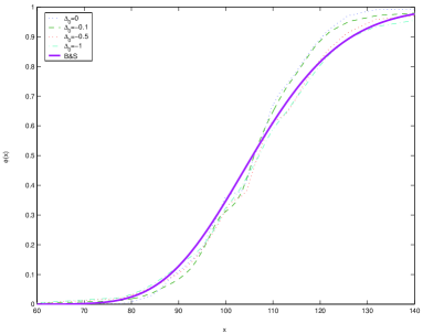
Figure 1: Optimal number of risky assets $\phi$ in the hedging portfolio, as a function of the level $x$ of the underlying asset for different strategies within the Black-Scholes. As expected the different curves are very similar. The value of the strike is $K=110$, and the time is half the maturity of the option: $k=N/2$.

This observation is confirmed by the shape of the distribution of the final wealth at the maturity date of the option, for the different strategies (Fig. 2).

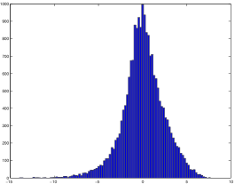
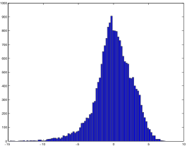
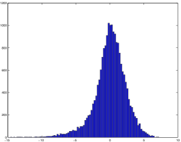
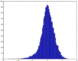
Figure 2: Distribution of the final wealth for different strategies for a BS market (upper left: BS, upper right: $\Delta_{0}=0$, lower left: $\Delta_{0}=-0.5$, lower right: $\Delta_{0}=-1$). The four curves are not very different from one another. The value of the strike is $K=110$.

3.3 The case of a fat-tailed dynamics

We are now interested in a market whose dynamics is governed by a fat tailed Lévy process, where the relative price increments are independent identically distributed with jumps. In this case the market is no longer complete (existence of unhedgeable jumps) and perfect replication does not exist. The use of a subjective criteria is then needed for pricing and hedging purposes, we now expect to get different strategies depending on the value of $\Delta_{0}$. Our expectations are numerically confirmed in Fig. 3 where we clearly see strong differences between the strategies. In particular, we observe that extreme losses hedging (corresponding to a large value of $|\Delta_{0}|$) leads to a flatter function $\phi(x)$ (i.e. a smaller Gamma). This was already emphasized in [23, 5] and can be quite interesting in presence of transaction costs (see section 4).

Figure 3: Optimal number of risky assets $\phi$ in the hedging portfolio, as a function of the level $x$ of the underlying asset for different strategies in the case of a fat tailed market (left: $\nu=6$ and right: $\nu=4$). The hedging strategies now present a very different dependence on the underlying, in particular when $|\Delta_{0}|$ increases. The value of the strike is $K=110$ and the time is half the maturity of the option: $k=N/2$.

Using an independent set of paths, we can check that our method indeed leads to smaller local expected shortfalls when the corresponding optimal strategy is adopted, as can be seen in Tables 1 and 2, where we give both the unconditional expected shortfall $\mathcal{R}$, and the conditional expected shortfall (noted ESF), defined as $\mathcal{R}/{\cal P}$, where ${\cal P}$ is the probability to exceed the threshold $\Delta_{0}$. These expected shortfalls are computed between two re-hedging times $k$ and $k+1$, where $k=N/2$ corresponds to half the life of the option.

strategy	BS	$\Delta_{0}=0$	$\Delta_{0}=-5$	$\Delta_{0}=-10$
ESF(0)	-0.77	-0.88	-0.93	-1.19
ESF(-5)	-2.26	-2.32	-2.17	-1.98
ESF(-10)	-4.38	-4.00	-3.05	-2.21
$\mathcal{R}(0)$	-0.22	-0.25	-0.33	-0.44
$\mathcal{R}(-5)$	-0.011	-0.014	-0.010	-0.015
$\mathcal{R}(-10)$	-0.002	-0.003	-0.002	-0.001

Table 1: Conditional expected shortfall (ESF) and unconditional expected shortfall $\mathcal{R}$, for different threshold $\Delta_{0}$ and different strategies, in the case $\nu=6$. These local quantities are computed for a time equal to half the maturity of the option (here 1 year), for a strike $K=110$.

strategy	BS	$\Delta_{0}=0$	$\Delta_{0}=-5$	$\Delta_{0}=-10$
ESF(0)	-0.88	-1.04	-1.04	-1.10
ESF(-5)	-4.45	-4.40	-3.94	-3.15
ESF(-10)	-8.58	-8.60	-7.76	-5.90
$\mathcal{R}(0)$	-0.23	-0.25	-0.35	-0.38
$\mathcal{R}(-5)$	-0.031	-0.035	-0.028	-0.028
$\mathcal{R}(-10)$	-0.015	-0.016	-0.011	-0.009

Table 2: Conditional expected shortfall (ESF) and unconditional expected shortfall $\mathcal{R}$, for different threshold $\Delta_{0}$ and different strategies, in the case $\nu=4$. These local quantities are computed for a time equal to half the maturity of the option (here 1 year), for a strike $K=110$.

We can also check that our method leads to satisfactory results for global quantities (i.e. concerning the wealth balance at the end of the option lifetime). We therefore determined the distribution of the final wealth (Fig. 4 and 5). We clearly see that the strategy proposed here can significantly reduce the value of the extreme losses (note that because of the power-tails of the return distribution, these extreme losses can still be large). Moreover we observe a remarkable change in the shape of this distribution: from relatively peaked for small $|\Delta_{0}|$ but with an appreciable number of extreme events, it becomes broader but with a smaller support when $|\Delta_{0}|$ increases. This fact can be qualitatively explained: when $|\Delta_{0}|$ is large, the constraint is easier to fulfill but losses of amplitude less than $|\Delta_{0}|$ are not penalized, leading to a broader looking but more sharply truncated final distribution.

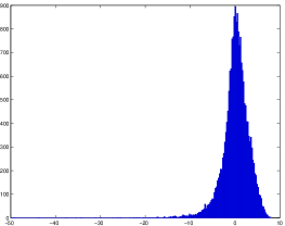
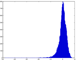
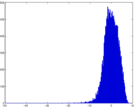
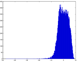
Figure 4: Distribution of the final wealth for different strategies in the case of a fat-tailed market with $\nu=6$ (upper left: BS, upper right: $\Delta_{0}=0$, lower left: $\Delta_{0}=-5$, lower right: $\Delta_{0}=-10$).

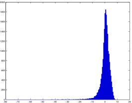
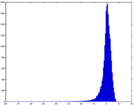
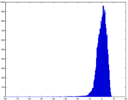
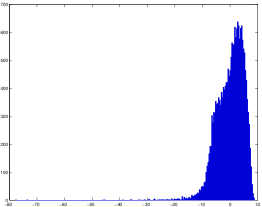
Figure 5: distribution of the final wealth for different strategies in the case of a fat-tailed market with $\nu=4$ (upper left: BS, upper right: $\Delta_{0}=0$, lower left: $\Delta_{0}=-5$, lower right: $\Delta_{0}=-10$).

We give in Tables 3 and 4 the mean and the standard deviation of these final wealth distributions, as well as the initial price of the option and the associated value at risk and expected shortfalls. Notice that the option price is smaller than the Black-Scholes price, which is expected when the moneyness is small: non zero kurtosis indeed leads to a decrease of the at-the-money volatility [5] as can be seen in Fig. 6. The option price in fact decreases when larger risks are hedged.

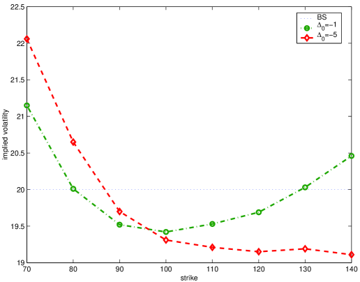
Figure 6: implied volatility smile at $t=0$. $\nu=4$ and $S_{0}=100$

strategy	BS	$\Delta_{0}=0$	$\Delta_{0}=-5$	$\Delta_{0}=-10$
option price	5.29	5.15	5.14	5.08
mean of final wealth	0.15	0.01	0.03	0.04
std of final wealth	3.11	3.23	3.41	4.01
VaR $0.1\%$	-21.81	-20.77	-19.04	-18.40
ESF $0.1\%$	-7.96	-8.50	-7.63	-6.73
VaR $1\%$	-10.04	-10.63	-8.82	-9.47
ESF $1\%$	-4.88	-4.91	-4.41	-3.69
VaR $5\%$	-4.85	-5.39	-5.28	-6.19
ESF $5\%$	-3.39	-3.46	-2.56	-2.28

Table 3: Statistical characteristics of the global wealth balance for $\nu=6$. The strike is $K=110$.

strategy	BS	$\Delta_{0}=0$	$\Delta_{0}=-5$	$\Delta_{0}=-10$
option price	5.29	5.08	4.99	4.89
mean of final wealth	0.29	0.09	0.07	0.09
std of final wealth	4.02	4.12	4.20	4.82
VaR $0.1\%$	-34.90	-36.49	-28.37	-27.45
ESF $0.1\%$	-16.14	-15.21	-14.05	-9.87
VaR $1\%$	-13.59	-14.28	-12.08	-12.72
ESF $1\%$	-9.34	-9.34	-7.85	-6.06
VaR $5\%$	-5.58	-6.19	-6.32	-7.76
ESF $5\%$	-5.48	-5.55	-4.23	-3.51

Table 4: Statistical characteristics of the global wealth balance for $\nu=4$. The strike is $K=110$.

4 Application to transaction costs

As mentioned above, hedging against extreme risks generically leads to a strategy that varies more slowly with the underlying asset price. This can be of great interest in the presence of transaction costs. These costs can in fact be endogenously taken into account within the present numerical scheme, which allows to determine how both the price and the optimal hedge are impacted by transaction costs. Previous analytical work on this problem in the framework of the BS model can be found in [27, 7], and further discussions and extensions to the case of non Gaussian markets can be found in [28].

We model friction by adding to the wealth balance a cost proportional to the number of bought or sold assets and to its price. Eq.1 now becomes

$$\Delta W_{k}=e^{\rho}\mathcal{C}_{k}(x_{k})-\mathcal{C}_{k+1}(x_{k+1})+\phi_{k}(x_{k})(x_{k+1}-e^{\rho}x_{k})-\beta x_{k}|\phi_{k}-\phi_{k-1}|,$$ (6)

where $\beta x_{k}$ represents the transaction costs per share. Following the same steps as above, we now want to minimize the risk function

$$\mathcal{R^{*}}_{k} = \sum_{\ell=1}^{N_{MC}}\bigg{(}\Delta_{0}-\left(e^{\rho}C_{k+1}(x_{k}^{\ell})-C_{k+1}(x_{k+1}^{\ell})\right)-(x_{k+1}^{\ell}-e^{\rho}x_{k}^{\ell})\phi_{k}(x_{k}^{\ell})$$

$$+\beta x_{k}^{\ell}|x_{k}^{\ell}-x_{k-1}^{\ell}|\frac{\partial\phi}{\partial x}(x_{k}^{\ell})\bigg{)}_{+},$$

where we approximated $|\phi_{k}-\phi_{k-1}|$ by $\frac{\partial\phi}{\partial x}|\Delta x|$. This is justified if the time step is sufficiently small, and is the key step to make the problem tractable. However, since this involves the derivative of $\phi$, we have preferred to work with a smooth parameterization of the function $\phi_{k}$ with only two optimization parameters, rather than the full decomposition over a set of basis functions, as was used above. We have checked that the following choice gives very similar results than the ones obtained above in the absence of transaction costs. We thus take:

$$\phi_{k}(x)=\frac{1}{2}\left(1+\left[\tanh\left|A_{k}{\cal M}_{k}\right|\right]^{\beta_{k}}.\text{sign}({\cal M}_{k})\right)$$

with a rescaled moneyness ${\cal M}_{k}$ given by:

$${\cal M}_{k}=\frac{x-Ke^{-r(T-t_{k})}}{\sigma\sqrt{T-t_{k}}}.$$

By varying the two variational parameters $A_{k}$ and $\beta_{k}$, we can, at each time step, optimize any risk measure. Using essentially the same numerical optimization procedure as above we are able to find the parameters $A_{k}$ and $\beta_{k}$, and thus the optimal strategy $\phi_{k}^{*}$. In order to obtain the option price, we have then to solve the following least square problem:

$$\min_{\gamma}\,\,\, \sum_{\ell=1}^{N_{MC}}\left[\sum_{a=1}^{p}\right.\gamma_{a}^{k}C_{a}^{k}(x_{k}^{\ell})-e^{-\rho}\bigg{(}\mathcal{C}_{k+1}(x_{k+1}^{\ell})-\phi_{k}(x_{k}^{\ell})(x_{k+1}^{\ell}-e^{\rho}x_{k}^{\ell})$$

$$\left.+\beta x_{k}^{\ell}|x_{k}^{\ell}-x_{k-1}^{\ell}|\frac{\partial\phi}{\partial x}(x_{k}^{\ell})\bigg{)}\right]^{2}$$

We have numerically tested the above scheme in the case of a BS market with the same characteristics as in the previous section, and for different values of the friction parameter $\beta$. We compared our results with those obtained following a naive BS strategy and the more advanced Leland strategy. Using simple arguments, similar in spirit to the above approximation on $\Delta\phi$, Leland showed in [27] how the BS strategy can be modified to account for transaction costs. Indeed using a modified volatility

$$\sigma_{L}=\sigma\sqrt{1+2\beta\sqrt{\frac{2}{\pi}}\frac{1}{\sigma\sqrt{\Delta t}}},$$

instead of the real volatility $\sigma$ leads to a strategy which, on average, approximately covers the transaction costs and hedges the risk. Since $\sigma_{L}>\sigma$, the option price is, as expected, higher than in the BS case. Figure 7 compares the obtained optimal strategies using our method with both the BS and Leland hedging schemes. As expected, the costs affects the BS strategy in such a way as to reduce its at the money Gamma. Tables 5, 6, 7 and 8 give a summary statistics of our results. We note that even in the case where the stock price is log-normal, our strategy allows to improve significantly over the Leland strategy if the threshold $|\Delta_{0}|$ is large enough: compare Tables 6 and 8. Using the optimal strategy allows one to simultaneously reduce the occurrence of large risks (measures both by the VaR and the ESF) while keeping the option price lower than in the Leland scheme.

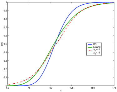
Figure 7: Optimal number of risky assets $\phi$ in the hedging portfolio, as a function of the level $x$ of the underlying asset for different strategies: Black-Scholes, Leland, $\Delta_{0}=-1$ and $\Delta_{0}=-5$, for $\beta=0.05$. The value of the strike is K=$110$.

$\beta$	0.005	0.01	0.05
option price	5.29	5.29	5.29
mean of final wealth	-0.41	-0.90	-4.78
std of final wealth	2.38	2.45	3.28
VaR $0.1\%$	-10.95	-11.86	-19.91
ESF $0.1\%$	-1.45	-1.47	-1.33
VaR $1\%$	-7.32	-8.06	-14.83
ESF $1\%$	-1.57	-1.67	-2.07
VaR $5\%$	-4.47	-5.15	-11.14
ESF $5\%$	-1.75	-1.84	-2.25

Table 5: Impact of the transaction costs for the B&S strategy.

$\beta$	0.005	0.01	0.05
option price	5.69	6.08	9.27
mean of final wealth	0.10	0.13	0.32
std of final wealth	2.39	2.44	2.98
VaR $0.1\%$	-9.83	-9.79	-10.32
ESF $0.1\%$	-1.54	-1.53	-1.28
VaR $1\%$	-6.47	-6.47	-6.83
ESF $1\%$	-1.55	-1.54	-1.60
VaR $5\%$	-3.80	-3.84	-4.27
ESF $5\%$	-1.67	-1.64	-1.62

Table 6: Impact of the transaction costs for the Leland strategy.

$\beta$	0.005	0.01	0.05
option price	5.77	6.22	8.30
mean of final wealth	0.00	-0.04	-0.26
std of final wealth	2.39	2.44	3.09
VaR $0.1\%$	-11.05	-10.95	-10.87
ESF $0.1\%$	-1.34	-1.45	-1.27
VaR $1\%$	-7.05	-7.13	-7.54
ESF $1\%$	-1.61	-1.54	-1.45
VaR $5\%$	-4.01	-4.11	-5.09
ESF $5\%$	-1.84	-1.80	-1.51

Table 7: Impact of the transaction costs using the optimal strategy, where these costs are accounted for. $\Delta_{0}=-1$

$\beta$	0.005	0.01	0.05
option price	5.63	5.99	8.44
mean of final wealth	0.00	-0.05	-0.75
std of final wealth	2.66	2.74	3.39
VaR $0.1\%$	-8.92	-9.17	-11.95
ESF $0.1\%$	-1.17	-1.27	-1.44
VaR $1\%$	-6.12	-6.37	-8.60
ESF $1\%$	-1.28	-1.31	-1.48
VaR $5\%$	-4.06	-4.25	-6.07
ESF $5\%$	-1.30	-1.33	-1.56

Table 8: Impact of the transaction costs using the optimal strategy, where these costs are accounted for. $\Delta_{0}=-5$

5 Conclusion

In this paper we have extended the work of [4] and proposed a general numerical (Monte-Carlo) methodology for the pricing and hedging of options when the market is incomplete, for an arbitrary risk criterion (chosen here to be the expected shortfall) and in the presence of transaction costs. We have shown that in the presence of fat-tails, our strategy allows to significantly reduce extreme risks, and generically leads to low Gamma hedging, as anticipated in [23, 5]. Many other risk criteria could be considered, in particular functions that give more weights to extreme losses. We focused in this work on plain vanilla European options, but (as shown in [4]) the method is readily extended to a large family of exotic options. Finally, we showed how our method allows to deal consistently with transaction costs. When compared to the standard Leland hedging scheme, our optimal strategy leads both to lower option prices and better hedging of large risks, even in the simplest case of a log-normal market.

There are many extensions of the above method that would be worth investigating, in particular the case where the underlying has a stochastic volatility with some persistence, such as, for example, the models studied in [12, 13, 14, 16, 18]. In this case, both the price and the optimal hedge should explicitly depend on the local value of the volatility, or of a noisy estimate of this volatility. Other hedging instruments, like options of different maturities, could in this case be included in the local wealth balance to reduce the risk further. Another interesting path is to consider the problem of hedging a whole portfolio of options. Contrarily to the Black-Scholes case, where the optimal strategy for the whole portfolio is the linear sum of the individual hedges, extreme value hedges lead to a non linear composition of the individual hedges.

References

- [1] F. Black and M. Scholes. The pricing of options and corporate liabilities. Journal of Political Economy, 81:637–654, 1973.
- [2] J.M. Harrison and S.R. Pliska. Martingales and stochastic integrals in the theory of continuous trading. Stochastic Processes and its Applications, 11:215–260, 1981.
- [3] M. Musiela and M. Rutkowski. Martingale methods in financial modelling. Springer, 1997.
- [4] M. Potters, J.-P. Bouchaud, and D. Sestovic. Hedged monte-carlo: low variance derivative pricing with objective probabilities. Physica A, 289:517–525, 2001.
- [5] J.-P. Bouchaud and M. Potters. Theory of financial risks. Cambridge University Press, 2000.
- [6] J.C. Hull. Options, futures and other derivatives. Prentice-Hall, 1997.
- [7] P. Wilmott. Derivatives. John Wiley & Sons, 1998.
- [8] S.I. Boyarchenko and S.Z. Levendorskii. Non-gaussian Merton-Black-Scholes Theory, volume 9 of Advanced Series on Statistical Science and Applied Probability. World Scientific, Singapore, edition, 2002. .
- [9] P. Carr, H. Geman, D. Madan, and M. Yor. Stochastic volatility for l evy processes. MathematicalFinance, 13(3):345–382, 2003.
- [10] E. Eberlein, U. Keller, and K. Prause. New insights into smile, mispricing and value at risk: the hyperbolic model. Journal of Business, 71:371–405, 1998.
- [11] E.M. Stein and J.C. Stein. Stock price distributions with stochastic volatility: An analytic approach. Review of Financial Studies, 4:727–752, 1991.
- [12] S.L. Heston. A closed-form solution for options xith stochastic volatility with applications to bond and currency options. Review of Financial Studies, 6:327–343, 1993.
- [13] A.A. Dragulescu and V.M. Yakovenko. Probability distribution of returns in the heston model with stochastic volatility. Quantitative Finance, 2(6):443–453, 2002.
- [14] J. Masoliver and J. Perelló. A correlated stochastic volatility model measuring leverage and other stylized facts. International Journal of Theoretical and Applied Finance, 5:541–562, 2002.
- [15] J. Perelló, J. Masoliver, and J.P. Bouchaud. Multiple time scales in volatility and leverage correlations: a stochastic volatility model. cond-mat/0302095, 2003.
- [16] J.F. Muzy, J. Delour, and E. Bacry. Modelling fluctuations of financial time series: from cascade process to stochastic volatility model. European Physic Journal B, 17:537, 2000.
- [17] L. Calvet and A. Fisher. Forecasting multifractal volatility. Journal of Econometrics, 105:27–58, 2001.
- [18] B. Pochart and J.-P. Bouchaud. The skewed multifractal random walk with applications to option smiles. Quantitative Finance, 2(4):303–314, 2002.
- [19] M. Schweizer. Mean-variance hedging for general claims. Annals of Applied Probability, 2:171–179, 1992.
- [20] P. Artzner, F. Delbaen, J.-M. Eber, and D. Heath. Coherent measures of risk. Mathematical Finance, 9:203–228, 1999.
- [21] H. Follmer and P. Leukert. Quantile hedging. Finance and Stochastics, 3(3):251–273, 1999.
- [22] R.T. Rockafellar and S. Uryasev. Optimization of conditional value-at-risk. The Journal of Risk, 2(3):21–41, 2000.
- [23] F. Selmi and J.-P. Bouchaud. Hedging large risks reduces transaction costs. Wilmott Magazine, :64, March 2003.
- [24] F.A. Longstaff and E.S. Shwartz. Valuing american options by simulation: a simple least-squares approach. Review of Financial Studies, 14(4):113–147, 2001.
- [25] W.T. Vetterling, S.A. Teukolsky, W.H. Press, and B.P. Flannery. Numerical recipes in C: the art of scientific computing. Cambridge University Press, 1993.
- [26] L. Borland. A theory of non-gaussian option pricing. Quantitative Finance, 2(6):415–431, 2002.
- [27] H.E. Leland. Option pricing and replication with transaction costs. Journal of Finance, 40:1283–1301, 1985.
- [28] F. Selmi. Quartic hedging schemes for options. PhD thesis, Université de Paris II-Assas, 2003. unpublished.