Dynamics of an anisotropic Haldane antiferromagnet in strong magnetic field

Abstract

We report the results of elastic and inelastic neutron scattering experiments on the Haldane-gap quantum antiferromagnet Ni(C₅D₁₄N₂)₂N₃(PF₆) performed at mK temperatures in a wide range of magnetic field applied parallel to the $S=1$ spin chains. Even though this geometry is closest to an ideal axially symmetric configuration, the Haldane gap closes at the critical field $H_{c}\simeq 4T$, but reopens again at higher fields. The field dependence of the two lowest magnon modes is experimentally studied and the results are compared with the predictions of several theoretical models. We conclude that of several existing theories, only the recently proposed model [Zheludev et al., cond-mat/0301424 ] is able to reproduce all the features observed experimentally for different field orientations.

I Introduction

The problem of field-induced magnon condensation in gapped quantum antiferromagnets is currently receiving a great deal of attention from experimentalists. Particularly important results were obtained in recent neutron scattering and ESR measurements on $S=1$ Haldane-gapHaldane (1983a, b) compounds Ni(C₂H₈N₂)₂NO₂(ClO₄) (NENP),End Ni(C₅D₁₄N₂)₂N₃(PF₆) (NDMAP) Honda et al. (1998, 1999); Chen et al. (2001); Zheludev et al. (2002); Zheludev+03 ; Hagiwara+03 and Ni(C₅H₁₄N₂)₂N₃(ClO₄) (NDMAZ),Zheludev2001-2 as well as the $S=\frac{1}{2}$-dimer system TlCuCl₃.Nikuni+00 ; Ruegg+02 ; Ruegg+03 The effect of magnetic field is to drive the gap $\Delta$ in such systems to zero by virtue of Zeeman effect, thus promoting a quantum phase transition to a new magnetized state at some critical value of the applied field $H_{c}\approx(\Delta/g\mu_{B})$.Katsumata+89 Additional magnetic anisotropy effects usually lead to more complex behavior and richer phase diagram. Anisotropy is negligible in many $S=\frac{1}{2}$-based materials such as TlCuCl₃, where no single-ion terms are possible. In contrast, for $S=1$ compounds such as NENP, NDMAP and NDMAZ, terms of type $DS_{z}^{2}$ are quite strong and the corresponding zero-field anisotropy splitting of the excitation triplet is comparable in magnitude to the Haldane gap itself. Under these circumstances, the physics is expected to depend strongly on the direction of the applied magnetic field with respect to the anisotropy axes.Golinelli et al. (1993)

For purely technical reasons, in quasi-1D materials it is much easier to perform inelastic neutron scattering experiments in high magnetic fields applied perpendicular to the spin chains. On most instruments the scattering plane is horizontal and the wave vector resolution along the vertical axis is deliberately coarsened to provide an intensity gain. To optimize wave vector resolution along the spin chains in the sample, and to allow the momentum transfer $q_{\parallel}\approx\pi$ in that direction, the chain axis has to be mounted in the horizontal plane. The typical construction of superconducting magnets is such that the field is along the vertical direction, and is thus applied perpendicular to the spin chains in the sample. In the Haldane-gap materials NENP, NDMAP and NDMAZ the anisotropy easy plane is roughly perpendicular the chains. As a result, most of the previous neutron measurements were performed for in-plane magnetic fields, i.e., in the Axially Asymmetric (AA) geometry. In the AA case the transition at $H_{c}$ is expected to be of Ising type,Tsvelik (1990); Affleck (1991) and even an isolated chain acquires antiferromagnetic long-range order in the ground state at $H>H_{c}$. The excitations in the magnetized state are a triplet of massive “breathers” (soliton-antisoliton bound states).Affleck (1991) Recent neutron scattering studies of NDMAP in the AA geometry provided a solid confirmation of these theoretical predictions.Zheludev+03

For an isolated Haldane spin chain magnetized in the Axially Symmetric (AS) geometry (with a magnetic field applied parallel to the anisotropy axis and the anisotropy being of a purely easy-plane type) theory predicts a totally different, disordered and quantum-critical ground state whose low-energy physics can be described as the Tomonaga-Luttinger spin liquid.Affleck (1991); Tsvelik (1990); Tak ; Sachdev+94 The low-energy excitation spectrum contains no sharp modes and is instead a continuum of states, much as for $S=\frac{1}{2}$ spin chains.Schulz+83-86 Higher modes which would have quasiparticle character in the AA geometry (two upper members of the Zeeman-split triplet) also develop into continua and exhibit only edge-type singularities in the AS case.KolezhukMikeska02 Moreover, one expects incommensurate correlations at a field-dependent Fermi wave vector that characterizes the Fermi sea of magnons “condensed” at $H>H_{c}$.Furusaki and Zhang (1999) In a real material this idealized picture may be complicated by several factors. First of all, there can be additional anisotropy terms, such as in-plane single-ion anisotropy or Dzyaloshinskii-Moriya interactions, which explicitly break the axial symmetry and favor the AA physics; a similar effect could be expected if the direction of the applied field deviates slightly from the symmetry axis. Residual three-dimensional inter-chain couplings lead to a spontaneous breaking of the axial symmetry which is equivalent to the Bose-Einstein condensation of magnons.Affleck (1991); Sachdev+94 ; GiamarchiTsvelik99 ; Nikuni+00 Due to the critical nature of the ground state of an isolated chain, all these effects are relevant and will have a significant impact on the spin correlations, no matter how small they may be. The key to understanding the high-field behavior in real materials is a combined approach involving high resolution neutron scattering experiments and a consistent theoretical treatment. Due to geometrical constraints described in the previous paragraph, high-field neutron measurements in the AS configuration are technically challenging and require the use of specialized neutron instruments or magnet environments.

The purpose of the present paper is twofold: on one hand, to study experimentally the response of the NDMAP system in the wide range of applied fields and at very low temperature, in the setup as close to the AS geometry as possible, and to test further the phenomenological field theory of the high-field phase which was recently proposed Zheludev+03 and successfully applied to the description of experiments on NDMAP in the AA geometry. Hagiwara+03 On the other hand, we also give a more detailed account of the theory which was only briefly outlined in Ref. Zheludev+03, , and generalize it to include the effect of interchain interactions. Finally, we perform a systematic quantitative comparison between our experimental findings and theoretical results.

The paper is organized as follows: in Sect. II we present the details of experimental setup, and Sect. III reports the results of elastic and inelastic neutron scattering measurements. In Sect. IV we present the general effective field theory of anisotropic gapped quasi-one-dimensional spin system in strong magnetic field and perform a systematic quantitative comparison between our experimental findings and theoretical results. Finally, Sect. V contains the summary and concluding remarks.

II Experimental setup

II.1 Structural considerations and energy scales

The crystal structure of NDMAP is schematically shown in Fig. 1 of Ref. Zheludev et al., 2001. The AF spin chains are composed of octahedrally-coordinated $S=1$ Ni²⁺ ions bridged by azido-groups. The chains run along the $c$ axis of the orthorhombic structure (space group $P{nmn}$, $a=18.046$ Å, $b=8.705$ Å, and $c=6.139$ Å). Previous zero-field neutron studies provided reliable estimates for the relevant magnetic energy scales in the system. The in-chain exchange constant is $J=2.6$ meV. Exchange coupling along the crystallographic $b$ axis is considerably weaker, $J_{b}/J\approx 10^{-3}$, and that along $a$ is weaker still, to the point of being undetectable: $|J_{a}/J|<10^{-4}$. Magnetic anisotropy in NDMAP is predominantly of single-ion easy-plane type with $D/J\approx 0.25$. In addition, there is a weak in-plane anisotropy term of type $E(S_{x}^{2}-S_{y}^{2})$. As a result of these anisotropy effects, at zero field the degeneracy of Haldane triplet is fully lifted and the gap energies are $\Delta_{1}=0.42(3)$ meV, $\Delta_{2}=0.52(6)$ meV, and $\Delta_{3}=1.9(1)$ meV. Correspondingly, the critical fields are strongly dependent on field orientation and the $H-T$ phase diagram, visualized in Fig. 1 is highly anisotropic.

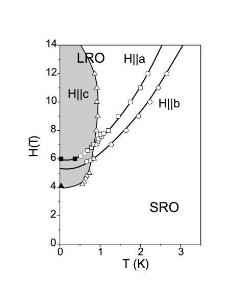
Figure 1: The $H-T$ phase diagram of NDMAP as deduced from specific heat measurements (open symbols, Ref. Honda et al., 1998) and neutron scattering experiments (solid symbols, Refs. Chen et al., 2001; Zheludev+03, and the present study). The shaded area is the high-field phase investigated in the present work.

The local anisotropy axes in NDMAP are determined by the geometry of the corresponding Ni²⁺ coordination octahedra and do not exactly coincide with crystallographic directions. Instead, the main axes of the NiN₆ octahedra are in the $(a,c)$ crystallographic plane, but tilted by $\alpha\approx 16^{\circ}$ relative to the $c$ axis. As illustrated in Fig. 2, within each chain, the tilts are in the same direction for all Ni²⁺-sites, so there is no intrinsic alternation in the chains, as is the case in many related compounds such as NENP. However, within the crystal structure there are two types of chains related by symmetry, and the corresponding tilt directions are opposite. This circumstance has a very important consequence for the present study. It implies that for NDMAP one can not apply the field along the anisotropy axis of all the magnetic ions in the sample. The closest one can come to this idealized AS scenario is by applying a field along the axis of bulk magnetic anisotropy, i.e., along the $(0,0,1)$ direction. In this case the field will form a small angle of $\pm\alpha$ with the local anisotropy axes for all spin chains.

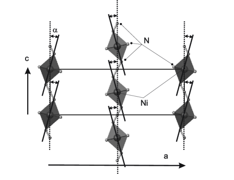
Figure 2: Main elements of the NDMAP crystal structure in projection onto the $(ac)$ crystallographic plane. Only the N and Ni sites are shown. Magnetic anisotropy associated with the Ni²⁺ magnetic ions is determined by the local symmetry of NiN₆ coordination tetrahedra that are tilted in the $(ac)$ plane by $\alpha=16^{\circ}$ relative to the $c$ axis. The tilt direction is opposite in adjacent chains.

II.2 Experimental procedures

Single-crystal neutron scattering experiments in magnetic fields applied parallel to the spin chains were carried out using two different setups. A series of diffraction measurements was carried out using a vertical-field 6 Tesla cryomagnet installed on the rather unique D23 lifting counter diffractometer at ILL. On this instrument the data collection is not restricted to a given scattering plane. The sample is mounted with the chain axis vertical (parallel to the field) and the detector is lifted out of the horizontal plane to allow a momentum transfers $q_{\parallel}\approx\pi$ in that direction. Neutrons of a fixed-incident energy $E_{i}=14.7$ mev were provided by a curved thermal neutron guide with supermirror coating, a Pyrolitic Graphite (PG) monochromator and a PG filter. In some cases horizontal and/or vertical collimators with a 40’ FWHM beam acceptance were inserted in front of the detector. In the diffraction study we employed a $\approx 0.3$ g fully deuterated single crystal sample.

Inelastic measurements were performed using the conventional 3-axis cold neutron spectrometer FLEX installed at HMI. An assembly of 3 deuterated single crystals with total mass about 1 g were mounted with chain axis in the horizontal (scattering) plane of the instrument. A magnetic field was applied along that direction by a horizontal-field cryomagnet. The data were collected with the final neutron energy fixed at 5 meV. A Be filter was used after the sample to eliminate higher-order beam contamination. Beam divergencies were defined by the critical angle of the cold-neutron guide, and by characteristics of the PG analyzer and monochromator used. No additional devices were used to collimate the neutron beams. In both the D23 and FLEX experiments the sample environment was a ³He-⁴He dilution refrigerator.

III Results of neutron scattering measurements

III.1 Magnetic long range order

Applying a field $H>H_{c}\approx 4.0$ T parallel to the $c$ axis at $T=25$ mK leads to antiferromagnetic long-range ordering in NDMAP. This was deduced from the appearance of new Bragg reflections at the 3D AF zone-centers $(h,k,l)+(0,-0.5,0.5)$, where $h$, $k$ and $l$ are integer. The measured field dependence of the (0,1.5,0.5) background-subtracted peak intensity is plotted in Fig. 3. In this data set the experimental error bars are too large to allow an accurate determination of $T_{N}$ and the order-parameter critical index.

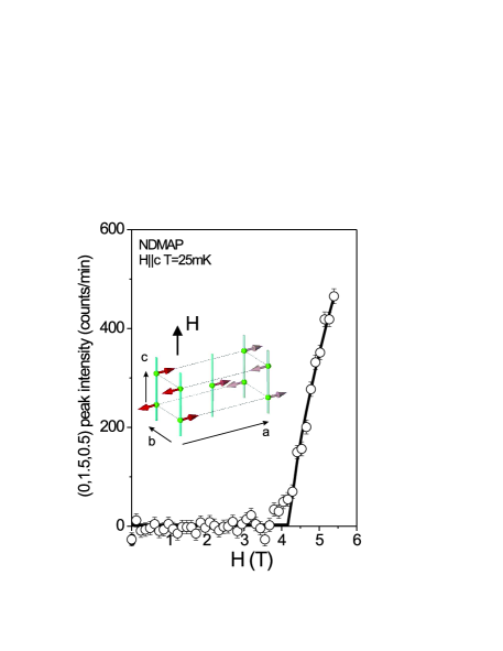
Figure 3: Measured peak intensity of the $(0,1.5,0.5)$ magnetic Bragg reflection in NDMAP as a function of magnetic field applied along the crystallographic $c$ axis (symbols). The solid line is a power-law fit to the data, that should only be viewed as a guide for the eye. Inset: proposed model for the spin structure in the high-field phase. Only the staggered magnetization probed by neutron diffraction is shown. In addition, a weak “ferromagnetic” tilt of all spins along the field direction is expected.

Fig. 4 shows $h$, $k$ and $l$ scans across the $(0,1.5,0.5)$ peak measured at $H=5.8$ T. These data were taken with a horizontal collimator installed in front of the detector, to improve wave vector resolution along the chain axis. The background was separately measured at $H=0$ and subtracted from the data shown. In all scans the magnetic peak width was determined to be resolution-limited. Thus, to within the experimental wave vector resolution, the high-field phase in NDMAP for $H\parallel c$ is characterized by true 3-dimensional long-range order.

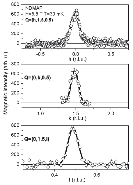
Figure 4: Elastic scans across the $(0,1.5,0.5)$ magnetic Bragg reflection in NDMAP at $T=30$ mK and $H=5.8$ T show resolution-limited peaks in all three directions. Solid lines are Gaussian fits to the data.

To determine the high-field spin arrangement, integrated intensities of 17 magnetic Bragg reflections were measured at $T=25$ mK and $H=5.8$ T using a standard diffraction configuration (no collimators). The observed intensity pattern is well reproduced by the simple model for the magnetic structure illustrated in the insert of Fig. 3. This spin arrangement is the same as previously seen for $\mathbf{H}\|[0\overline{1},1]$.Chen et al. (2001) The collinear model is clearly oversimplified, and the actual structure should be a canted one, with all spins slightly tilted towards the field and thus producing a net magnetization along that direction. In our experiment we can detect only the staggered part $\vec{L}$ of the magnetic moment which lies, within the experimental accuracy, along the crystallographic $a$ axis, perpendicular to the field direction. The local spin directions are opposite on sites related by $(0,1,0)$ and $(0,0,1)$ translations, and the same on sites related by a translation along $(1,0,0)$. Comparing the experimentally determined intensities of nuclear and magnetic reflections provides an estimate for the total staggered magnetization per site: $L=0.9(1)$ $\mu_{\mathrm{B}}$. This experimental value is about half of the classical sublattice magnetization for an ordered $S=1$ system.

III.2 Inelastic scattering

III.2.1 Constant-$q$ data

The field dependence of the gap energies was measured in a series of energy scans performed at the 1D AF zone-center $(0,k,0.5)$. The scans corresponded to a fixed momentum transfer parallel to the chains $q_{\parallel}=\pi/c$. The wave vector transfer perpendicular to the chains $q_{\perp}=2\pi k/b$ was varied in the course of the scan to satisfy geometrical restrictions imposed by the construction of the horizontal-field magnet. The background for all scans was measured at $H=0$ and $H=6$ T, away from the 1D AF zone-center, at $\mathbf{q}=(0,k,0.33)$. Apart from the expected elastic contribution due to incoherent scattering, the background was found to be energy-independent and about 1.5 counts/min. Typical background-removed scans collected at $H=1$ T$<H_{c}$, $H=4.1$ T$\approx H_{c}$ and $H=6$ T$>H_{c}$ are shown in Fig. 5 (symbols).

Figure 5: Typical background-subtracted constant-$q_{\parallel}$ scans measured in NDMAP up to 1.75 meV energy transfer for different values of magnetic field applied along the crystallographic $c$ axis (symbols). The two peaks are the lower-energy members of the Haldane excitation triplet. The third mode has a larger gap and is outside the shown scan range. Solid lines are fits to the data using a single-mode model cross section, as described in the text.

Scans collected at all fields are combined in the 3D plot shown in Fig. 6. The data were analyzed using a single-mode cross section function similar to that used in Ref. Zheludev et al., 2001:

$$S_{j}(\mathbf{q},\omega) \propto |f(q)|^{2}P_{j}\frac{1-\cos(\mathbf{q}\mathbf{c})}{2\omega_{j,\mathbf{q}}}\times$$ (1)

$$\times \left[\delta(\hbar\omega-\hbar\omega_{j,\mathbf{q}})+\delta(\hbar\omega+\hbar\omega_{j,\mathbf{q}})\right]$$

$$(\hbar\omega_{j,\mathbf{q}})^{2} = \Delta_{j}^{2}+v^{2}\sin^{2}(\mathbf{q}\mathbf{c}).$$ (2)

Here $j={1,2,3}$ labels each of the three excitation branches, $v$ is the spin wave velocity, $f(q)$ is the magnetic form factor for Ni²⁺, and $\Delta_{j}$ are the gap energies. The intensity prefactors $P_{j}$ depend on both the matrix elements between the ground state and the single-mode excited states and on the polarization of the latter. The model cross section was numerically convoluted with the calculated spectrometer resolution function. The gap energies and prefactors for each mode were refined using a least-squares routine to best-fit the data collected at each field. The spin wave velocity was fixed at $v=6.5$ meV, as determined previously for $H=0$.Zheludev+03 The resulting fits are represented by the solid lines in Figs. 5 and 6. The shaded areas in Fig. 5 are partial the contributions of each mode. The obtained field dependence of the energy gap is plotted in the $(H,\hbar\omega)$ plane of the 3D plot in Fig. 6 and, in more detail, in the top panel of Fig. 8. We have observed only two lower-energy members of the Haldane excitation triplet; the third mode has a larger gap and is outside the shown scan range. The field dependence of the upper two triplet modes was observed in recent ESR measurements.Hagiwara+03 However, the lowest triplet mode was not observed in Ref. Hagiwara+03, since those measurements were done at much higher temperature $T=1.5$ K where the lowest mode becomes strongly damped, the situation similar to that encountered in our early experiments in the $H\parallel a$ geometry which were also done at high temperature and failed to observe the reopening of the gap in the lowest mode.

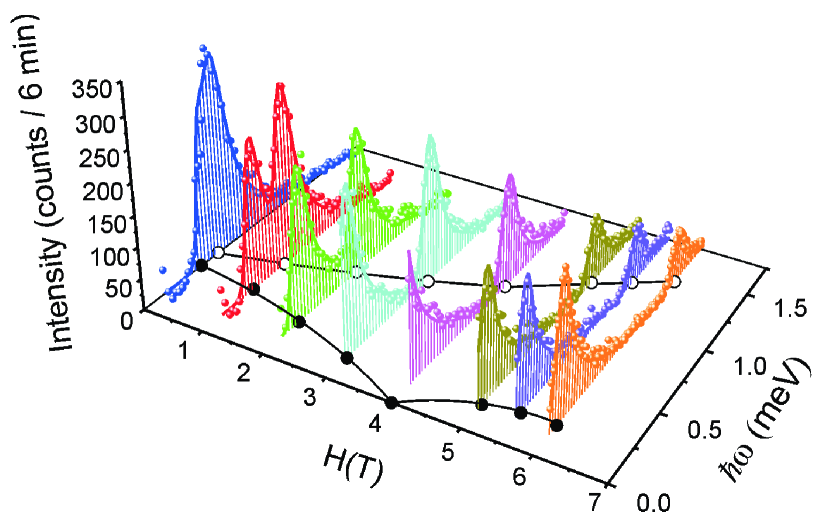
Figure 6: Background-subtracted constant-$q_{\parallel}$ scans measured in NDMAP for different values of magnetic field applied along the crystallographic $c$ axis. Solid lines and shaded areas are fits to the data using a model cross section function, as described in the text. The black and white circles in the $(H,\hbar\omega)$ plane are the measured field dependence of the two lower energy gaps in NDMAP. The connecting solid lines are guides for the eye.

Figure 7: Background-subtracted constant-$E$ scans measured in NDMAP for different values of magnetic field applied along the crystallographic $c$ axis (color symbols). Solid lines and shaded areas are simulations using a single-mode cross section function and parameters obtained in the analysis of const-$q_{\parallel}$ scans, as described in the text.

III.2.2 Constant-$E$ scans

As mentioned in the introduction, theory predicts that the spectrum at $H>H_{c}$ in the ideal AS geometry should lose its single-mode character. The sharp magnon excitations are expected to be replaced by a diffuse continuum of states with a lower bound following the magnon dispersion curve. Even in this case, the continuum is singular at the lower bound and may be difficult to distinguish from a single-mode excitation smeared effects of experimental resolution.

In search for any deviations from the single-mode picture we performed constant-$E$ scans at 1.8 meV (Fig. 7) and 1.2 meV (not shown) at $H=2$ T$<H_{c}$, $H=4$ T$\approx H_{c}$ and $H=6$ T$>H_{c}$. These particular energies were selected to avoid both gap energies at all three field values. A constant background was assumed for each scan. At each field, a single-mode profile was simulated using the model cross-section function described above, with parameter values obtained in the analysis of const-$q_{\parallel}$ data. We found that, to within experimental error, the single-mode model (solid lines in Fig. 7) reproduces all measured const-$E$ scans very well, below, at and above $H_{c}$. The observed variation of scan shape is due to changes in the gap energies of the two lower modes, shown as shaded areas in Fig. 7. No features beyond those given by the single-mode approximation could be detected with the resolution of the present study.

IV Anisotropic gapped quasi-1D spin system in strong magnetic field: theory

We now turn to developing a theoretical model of the high-field state. Our goal is a semi-quantitative effective field theoretical description, backed by a simple physical picture, yet capable of consistently reproducing all the available experimental data on NDMAP. The latter implies that the model should account for both neutron and ESR measurements,Honda et al. (1999); Hagiwara+03 work both above and below the critical field, and apply in the case of arbitrary field orientation.

IV.1 A single anisotropic Haldane chain in a field

IV.1.1 Existing models

In the early 90s, several phenomenological field-theoretical descriptions of the high-field regime in the anisotropic Haldane chain were proposed.Affleck (1990, 1991); Tsvelik (1990); Mitra and Halperin (1994) Affleck Affleck (1990, 1991) proposed a theory based on coarse-graining the $O(3)$ nonlinear sigma model (NLSM).Haldane (1983a, b) Technically coarse-graining leads to relaxing the unit vector constraint of the NLSM, so that one has a theory of unconstrained real vector bosonic field $\bm{\varphi}$. The $\varphi^{4}$-type interaction was added to ensure stability in the high-field regime, and the anisotropy was introduced just by assuming three different masses $\Delta_{\alpha}$ for the three field components, so that the resulting Lagrangian had the form

$$\mathcal{L} = \frac{1}{2v}\Big{\{}(\partial_{t}\bm{\varphi}+\bm{H}\times\bm{\varphi})^{2}-v^{2}(\partial_{x}\bm{\varphi})^{2}$$ (3)

$$- \sum_{\alpha}\Delta_{\alpha}\varphi_{\alpha}^{2}-\lambda(\bm{\varphi}^{2})^{2}\Big{\}}.$$

For $H>H_{c}$ the ground state acquires a nonzero staggered magnetization $\bm{L}=\langle\bm{\varphi}\rangle$ and a uniform magnetization $\bm{M}\propto\langle\bm{H}\times\bm{\varphi}\rangle$. This model captures the basic physics involved, but is known to suffer from several drawbacks. Because of the too simplistic way of introducing the anisotropy, the predicted values of the critical field ($H_{c}^{(\alpha)}=\Delta_{\alpha}$ for the field $\bm{H}$ directed along one of the symmetry axes $\bm{e}_{\alpha}$) disagree with the results of perturbative treatment Golinelli et al. (1992, 1993); Regnault et al. (1993) as well as with the experimental data on the behavior of gaps as functions of the applied field in NENP Regnault et al. (1994) and NDMAP.Zheludev+03

Tsvelik Tsvelik (1990) proposed a different theory which stems from the integrable Takhtajan-Babujian model of a $S=1$ chain and involves three Majorana fields with masses $\Delta_{\alpha}$. The theory yields the critical field value $H_{c}^{(\alpha)}=\sqrt{\Delta_{\beta}\Delta_{\gamma}}$ which coincides with the perturbative formulas of Golinelli et al. (1992, 1993); Regnault et al. (1993). This model was rather successful for the description of the field dependencies of the gaps below $H_{c}$ in NENP,Regnault et al. (1994) and is expected to yield a correct critical behavior at $H\to H_{c}$. However, when the high-field neutron data on NDMAP in the $H\parallel a$ geometry became available, Zheludev+03 it turned out that Tsvelik’s theory, apart from overestimating the $H_{c}$ value considerably, predicts no change of slope for the two upper magnon modes at $H=H_{c}$, in complete disagreement with the experimental data. One may conclude that though this model correctly describes the behavior of the low-energy degrees of freedom near the critical field, but fails to describe the behavior of high-energy modes above $H_{c}$.

Mitra and Halperin Mitra and Halperin (1994) have modified Affleck’s bosonic Lagrangian in order to reproduce Tsvelik’s results for the gaps. It turns out that changing the first term in (3) to

$$\frac{1}{2v}\sum_{\alpha}\big{\{}\partial_{t}\varphi_{\alpha}+\sum_{\beta\gamma}(\Delta_{\gamma}/\Delta_{\alpha})^{1/2}\epsilon_{\alpha\beta\gamma}H_{\beta}\varphi_{\gamma}\big{\}}^{2}$$ (4)

exactly reproduces the results of Ref. Tsvelik, 1990 for the field dependencies of the gaps below $H_{c}$. Above $H_{c}$, the predicted field behavior of the gaps is different from that of Ref. Tsvelik, 1990, and is in a reasonable qualitative agreement with the experimental data on NDMAP in the $H\parallel a$ geometry.Zheludev+03 However, apart from the fact that the reasons for the postulated modification (4) remain unclear, the theory still has one fundamental flaw: it predicts that the staggered moment at $H>H_{c}$ is directed along the magnetic hard axis $c$ for $H\parallel a$ and along the intermediate axis $b$ for $H\parallel c$. This result is not only counter-intuitive but also contradicts to the diffraction experiments on NDMAP Chen et al. (2001) which show that the ordered moment, in complete analogy to the classical picture for an ordered antiferromagnet, always lies in the easy plane along the most easy axis perpendicular to the field, i.e., along the $b$ axis for $H\parallel a$ and along the $a$ axis in the $H\parallel c$ case.

IV.1.2 An improved model

We see that none of the previously known models provides a consistent description of the experimental data. We use a different, more general approach, based on the model proposed in Ref. Kolezhuk, 1996 for dimerized $S=1/2$ chains and $S=1/2$ ladders, known to be in the same universality class as $S=1$ Haldane chains. This model was recently applied with great success to the description of the INS data for NDMAP in the $H\parallel a$ geometry,Zheludev+03 and to ESR experiments in both geometries.Hagiwara+03

We first illustrate the general features of the theory on the example of the alternated $S=\frac{1}{2}$ chain consisting of weakly coupled anisotropic dimers, described by the Hamiltonian

$${\mathcal{H}}=\sum_{n\alpha}J_{\alpha}S_{2n-1}^{\alpha}S_{2n}^{\alpha}+\sum_{n}\{J^{\prime}(\vec{S}_{2n}\cdot\vec{S}_{2n+1})-\vec{H}\cdot\vec{S}_{n}\},$$ (5)

where $0<J^{\prime}\ll J$. Throughout the rest of this section, it is implied that the magnetic field is measured in energy units, i.e., $H\mapsto g\mu_{B}H$ unless explicitly stated otherwise. For the derivation of the effective field theory it is convenient to use the dimer coherent states Kolezhuk (1996)

$$|\vec{A},\vec{B}\rangle=(1-A^{2}-B^{2})^{1/2}|s\rangle+\sum_{j}(A_{j}+iB_{j})|t_{j}\rangle,$$ (6)

where the singlet state $|s\rangle$ and three triplet states $|t_{j}\rangle$ are given by SachdevBhatt90

$$|s\rangle=\frac{1}{\sqrt{2}}\big{(}|\uparrow\downarrow\rangle-|\downarrow\uparrow\rangle\big{)}, |t_{z}\rangle=\frac{1}{\sqrt{2}}\big{(}|\uparrow\downarrow\rangle+|\downarrow\uparrow\rangle\big{)},$$

$$|t_{x}\rangle=-\frac{1}{\sqrt{2}}\big{(}|\uparrow\uparrow\rangle-|\downarrow\downarrow\rangle\big{)}, |t_{y}\rangle=\frac{i}{\sqrt{2}}\big{(}|\uparrow\uparrow\rangle+|\downarrow\downarrow\rangle\big{)},$$

and $\vec{A}$, $\vec{B}$ are real vectors which are in a simple manner connected with the magnetization $\vec{M}=\langle\vec{S}_{1}+\vec{S}_{2}\rangle$ and sublattice magnetization $\vec{L}=\langle\vec{S}_{1}-\vec{S}_{2}\rangle$ of the spin dimer:

$$\vec{M}=2(\vec{A}\times\vec{B})\;,\quad\vec{L}=2(1-A^{2}-B^{2})^{1/2}\vec{A}\;.$$ (7)

The configuration space is the inner domain of the unit sphere $\vec{A}^{2}+\vec{B}^{2}\leq 1$ in $R^{6}$, with additional identification of the opposite points on the sphere, and the measure is defined as $6\pi^{-3}d\vec{A}\;d\vec{B}$.

We will assume that we are not too far above the critical field, so that the magnitude of the triplet components is small, $A,B\ll 1$. Then the effective Lagrangian density in the continuum limit takes the following form:

$${\mathcal{L}} = -2\hbar\vec{B}\cdot\partial_{t}\vec{A}-\frac{1}{2}J^{\prime}\ell^{2}(\partial_{x}\vec{A})^{2}-\sum_{i}\{m_{i}A_{i}^{2}+\widetilde{m}_{i}B_{i}^{2}\}$$ (8)

$$+ 2\vec{H}\cdot(\vec{A}\times\vec{B})-U_{4}(\vec{A},\vec{B}),$$

where $m_{i}=\widetilde{m}_{i}-J^{\prime}$, $\ell$ is the lattice constant, and $\widetilde{m}_{i}=\frac{1}{4}|\epsilon_{ijn}|(J_{j}+J_{n})$. The fourth-order term

$$V_{4}(\vec{A},\vec{B})=\lambda(\vec{A}^{2})^{2}+\lambda_{1}(\vec{A}^{2}\vec{B}^{2})+\lambda_{2}(\vec{A}\cdot\vec{B})^{2},$$ (9)

where $\lambda=J^{\prime}$, $\lambda_{1}=2J^{\prime}$, $\lambda_{2}=-J^{\prime}$ in the present case. The spatial derivatives of $\vec{B}$ are omitted in (8) because they appear only in terms which are of the fourth order in $\vec{A}$, $\vec{B}$. Generally, we can assume that spatial derivatives are small (small wave vectors), but we shall not assume that the time derivatives (frequencies) are small since we are going to describe high-frequency modes as well.

The vector $\vec{B}$ can be integrated out, and under the assumption $A\ll 1$ it can be expressed through $\vec{A}$ as follows:

$$\vec{B}=\widehat{Q}\vec{F},\quad\vec{F}=-\hbar\partial_{t}\vec{A}+(\vec{H}\times\vec{A})$$ (10)

$$Q_{ij}={\delta_{ij}\over\widetilde{m}_{i}}-\lambda_{2}{A_{i}A_{j}\over\widetilde{m}_{i}\widetilde{m}_{j}}.$$

After substituting this expression back into (8) one obtains the effective Lagrangian depending on $\vec{A}$ only:

$${\mathcal{L}} = {1\over\widetilde{m}_{i}}\hbar^{2}(\partial_{t}A_{i})^{2}-v_{i}^{2}\ell^{2}(\partial_{x}A_{i})^{2}\Big{\}}$$

$$- 2{\hbar\over\widetilde{m}_{i}}(\vec{H}\times\vec{A})_{i}\partial_{t}A_{i}-U_{2}(\vec{A})-U_{4}(\vec{A},\partial_{t}\vec{A}),$$

where $v_{i}=\sqrt{J^{\prime}\widetilde{m}_{i}/2}$ are the characteristic velocities in energy units, and the quadratic and quartic parts of the potential are given by

$$U_{2}(\vec{A})=m_{i}A_{i}^{2}-{1\over\widetilde{m}_{i}}(\vec{H}\times\vec{A})_{i}^{2},$$ (12)

$$U_{4}(\vec{A},\partial_{t}\vec{A})=\lambda(\vec{A}^{2})^{2}+\lambda_{1}\vec{A}^{2}{1\over\widetilde{m}_{i}^{2}}F_{i}^{2}+\lambda_{2}{A_{i}A_{j}\over\widetilde{m}_{i}\widetilde{m}_{j}}F_{i}F_{j}$$

Note that the cubic in $\vec{A}$ term in (10) must be kept since it contributes to the $U_{4}$ potential.

Having in mind that the alternated $S={1\over 2}$ chain and the Haldane chain belong to the same universality class, one may now try to apply this model in the form (IV.1.2-12) to the Haldane chain system such as NDMAP, treating the velocities $v_{i}$ and interaction constants $m_{i}$, $\widetilde{m}_{i}$, $\lambda$, and $\lambda_{1,2}$ as phenomenological parameters.

One can show that the Lagrangian (IV.1.2) contains theories of Affleck Affleck (1990, 1991) and Mitra and Halperin Mitra and Halperin (1994) as particular cases. Indeed, restricting the interaction to the simplified form with $\lambda_{1,2}=0$ and assuming isotropic velocities $v_{i}=v$, one can see that the Affleck’s Lagrangian (3) corresponds to the isotropic $\vec{B}$-stiffness $\widetilde{m}_{i}=\widetilde{m}$, while another choice $\widetilde{m}_{i}=m_{i}$ yields the modification (4).

For illustration, let us assume that $\vec{H}\parallel z$. Then the quadratic part of the potential takes the form

$$U_{2}=(m_{x}-{H^{2}\over\widetilde{m}_{y}})A_{x}^{2}+(m_{y}-{H^{2}\over\widetilde{m}_{x}})A_{y}^{2}+m_{z}A_{z}^{2},$$ (13)

and the critical field is obviously $H_{c}=\min\{(m_{x}\widetilde{m}_{y})^{1/2},(m_{y}\widetilde{m}_{x})^{1/2}\}$. At zero field the three triplet gaps are given by $\Delta_{i}=(m_{i}\widetilde{m}_{i})^{1/2}$. Below $H_{c}$ the energy gap for the mode polarized along the field stays constant, $\hbar\omega_{z}=\Delta_{z}$, while the gaps for the other two modes are given by

$$(\hbar\omega_{xy}^{\pm})^{2} = {1\over 2}(\Delta_{x}^{2}+\Delta_{y}^{2})+H^{2}$$

$$\pm \Big{[}(\Delta_{x}^{2}-\Delta_{y}^{2})^{2}+H^{2}(m_{x}+m_{y})(\widetilde{m}_{x}+\widetilde{m}_{y})\Big{]}^{1/2}.$$

Below $H_{c}$ the mode energies do not depend on the interaction constants $\lambda_{i}$.

It is easy to see that in the special case $m_{i}=\widetilde{m}_{i}$, the above expression transforms into

$$\hbar\omega_{xy}^{\pm}={1\over 2}(\Delta_{x}+\Delta_{y})\pm\Big{[}{1\over 4}(\Delta_{x}-\Delta_{y})^{2}+H^{2}\Big{]}^{1/2},$$ (15)

which exactly coincides with the formulas obtained in the approach of Tsvelik, Tsvelik (1990) and also with the perturbative formulas of Ref. Golinelli et al., 1992, 1993; Regnault et al., 1993 and with the results of modified bosonic theory of Mitra and Halperin. Mitra and Halperin (1994) The peculiarity of this special choice of parameters is that above $H_{c}=(m_{x}m_{y})^{1/2}$ the most negative eigenvalue of the quadratic form (13) corresponds not to the component of $\vec{A}$ along the easy axis in the $(xy)$ plane, as one would intuitively expect, but to the component along the harder axis. For instance, if $x$ is the easy axis, $m_{x}<m_{y}$, then the most negative coefficient will be that at $A_{y}$. This leads to the above-mentioned problem with counter-intuitive direction of the ordered moment in the theory of Mitra and Halperin.

Generally, at $H>H_{c}$ one has to find the minimum of the static part of the potential and linearize the theory around the new static solution $\vec{A}=\vec{A}^{(0)}$. The equations for $\vec{A}^{(0)}$ have the form

$$\sum_{j}\Omega_{\beta j}A_{j}+\sum_{imn}\Lambda_{\beta i,mn}A_{i}A_{m}A_{n}=0,$$ (16)

where the matrices $\mathsf{\Omega}$, $\mathsf{\Lambda}$ are defined as

$$\Omega_{ij}=m_{i}\delta_{ij}-\sum_{kln}\epsilon_{ikn}\epsilon_{jln}\frac{1}{\widetilde{m}_{n}}H_{k}H_{l},$$

$$\Lambda_{ij,mn}=\Gamma_{ij,mn}+\Gamma_{mn,ij},$$ (17)

$$\Gamma_{ij,mn}=\lambda\delta_{ij}\delta_{mn}+(\lambda_{1}\delta_{ij}+\lambda_{2})\sum_{kl}\epsilon_{ikn}\epsilon_{jlm}\frac{H_{k}H_{l}}{\widetilde{m}_{i}\widetilde{m}_{j}}.$$

The magnon energies $\hbar\omega$ as functions of the field $H$ and of the longitudinal (with respect to the chain direction) wave vector $q$ can be found as three real roots of the secular equation

$$\det(\mathsf{M}-(\hbar\omega)^{2}\mathsf{G}-i\hbar\omega\mathsf{C})=0,$$ (18)

where symmetric matrices $\mathsf{M}$ and $\mathsf{G}$ are given by

$$M_{ij} = \Omega_{ij}+\frac{(v_{i}q\ell)^{2}}{\widetilde{m}_{i}}\delta_{ij}$$

$$+ \sum_{mn}A_{m}^{(0)}A_{n}^{(0)}(\Lambda_{ij,mn}+\Lambda_{im,jn}+\Lambda_{in,mj}),$$

$$G_{ij} = \left\{\frac{1}{\widetilde{m}_{i}}-\lambda_{1}\Big{(}\frac{A_{i}^{(0)}}{\widetilde{m}_{i}}\Big{)}^{2}\right\}\delta_{ij}-\lambda_{2}\frac{A_{i}^{(0)}A_{j}^{(0)}}{\widetilde{m}_{i}\widetilde{m}_{j}},$$ (19)

and the antisymmetric matrix $\mathsf{C}=\mathsf{R}-\mathsf{R}^{T}$ is determined by

$$R_{ij} = \left\{\frac{1}{\widetilde{m}_{i}}-\lambda_{1}\Big{(}\frac{A_{i}^{(0)}}{\widetilde{m}_{i}}\Big{)}^{2}\right\}\sum_{l}\epsilon_{ijl}H_{l}$$ (20)

$$+ \lambda_{2}\frac{A_{i}^{(0)}}{\widetilde{m}_{i}}\sum_{ln}\Big{\{}\frac{1}{\widetilde{m}_{j}}-\frac{1}{\widetilde{m}_{n}}\Big{\}}\epsilon_{jln}A_{n}^{(0)}H_{l}.$$

Here in case of NDMAP the longitudinal wave vector $q$ must be understood as counted from the 1D Bragg point, $q\ell\mapsto q_{\parallel}c-\pi$.

IV.2 Inter-chain interactions

Up to now, we have treated the problem as purely one-dimensional. In NDMAP, however, antiferromagnetic interchain interactions along the crystallographic $b$ direction lead to an observable transverse dispersion with the bandwidth of about $0.1$ meV.Zheludev et al. (2001) This value is small compared to the magnon bandwidth along the chain axis ($\simeq 7$ meV), but constitutes approximately 20% of the lowest magnon gap, so that transverse interactions have to be taken into account if one aims at a quantitative description.

It is straightforward to incorporate this effect into our formalism. Additional coupling of the form

$$J_{\perp}\sum_{j}(\vec{A}_{j}\cdot\vec{A}_{j+1}),$$ (21)

where $j$ labels chains along the transverse $b$-direction, amounts to a renormalization of the $\vec{A}$-stiffnesses $m_{\alpha}\mapsto m_{\alpha}+2J_{\perp}\cos(q_{\perp}b)$. The minimum of magnon energies is reached at the 3D AF zone center, in our case at $q_{\parallel}c=q_{\perp}b=\pi$. It is convenient to redefine the stiffness $m_{\alpha}$ as its value at the zone center $m_{\alpha}(q_{\perp}=\pi/b)$, so that in the formulas (16)-(20) one just has to make the substitution

$$m_{\alpha}\mapsto m_{\alpha}+2J_{\perp}(1+\cos q_{\perp}b).$$

Secular equations (18) then yield magnon energies for an arbitrary transverse wave vector transfer.

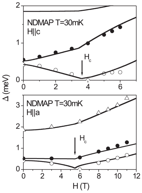
Figure 8: Symbols: measured field dependence of the energy gaps in NDMAP for a magnetic field applied along the crystallographic $c$-axis (top, this work) and $a$-axis (bottom, Ref. Zheludev+03, ). Lines: a global fit to the experimental data based on the Ginsburg-Landau type model outlined in Ref. Zheludev+03, and described in detail in the text. Note the different scales on the top and bottom figures.

IV.3 Comparison with experiment

The main advantage of the described model is that it can consistently reproduce all the experimental data currently available for NDMAP. At a first glance, it may appear over-parameterized, with 9 separate phenomenological constants: $m_{\alpha}$, $\widetilde{m}_{\alpha}$, $\lambda$, $\lambda_{1}$ and $\lambda_{2}$. However, all these parameters are relevant and can be almost uniquely determined from the measured field dependencies of the gap energies. Indeed, as discussed above, the independently measured zero-field gaps $\Delta_{\alpha}$ fix three relations $\Delta_{\alpha}^{2}=m_{\alpha}\widetilde{m}_{\alpha}$. The value of the critical field $H_{c}^{(\alpha)}$ for a field applied along the principal anisotropy axis $\alpha$ determines another three relations between parameters, namely $(H_{c}^{(\alpha)})^{2}=\min(m_{\beta}\widetilde{m}_{\gamma},m_{\gamma}\widetilde{m}_{\beta})$. One can show that of those six equations for six stiffness constants $m_{\alpha}$ and $\widetilde{m}_{\alpha}$ only five are independent, so that all stiffness constants can be expressed through one of them (we have chosen $m_{x}$ for this role). Finally, the interaction parameters $\lambda$, $\lambda_{1,2}$ control the behavior of the gap energies above the critical fields. In fact, the gaps depend only on the relative interaction strengths $(\lambda_{1}/\lambda)$, $(\lambda_{2}/\lambda)$, so that the scale of $\lambda$ does not influence the expressions for the gaps and can be set deliberately (we have put $\lambda=1$). Thus, the knowledge of the $H=0$ gaps and of critical fields helps to fix five parameters, and one parameter turns out to be irrelevant, so that one is left with only three parameters to fit the $\Delta(H)$ curves.

In analyzing the measured field dependencies of the gap energies in NDMAP, one has to keep in mind that both for the experiments described here, and for those reported in Ref. Zheludev+03, for $H\parallel a$, the transverse wave vector $q_{\perp}=2\pi k/b$ is not constant, but varies as a function of energy transfer $\hbar\omega$. For $H\parallel c$, $q_{\perp}$ is dictated by the geometry of the horizontal-field magnet, $q_{\perp}b/(2\pi)=0.42\,{\rm meV}^{-1}\times(\hbar\omega)$. In the $H\parallel a$ experiment of Ref. Zheludev+03, $q_{\perp}$ was chosen to optimize wave vector resolution along the chains when using a horizontally focusing analyzer, $q_{\perp}b/(2\pi)=1.3+0.24\,{\rm meV}^{-1}\times(\hbar\omega)$. In both cases the presence of inter-chain interactions must be taken into account explicitly, as discussed in the previous subsection. The value of $4J_{\perp}$ was chosen to match the transverse dispersion bandwidth of $0.1$ meV observed in NDMAP Zheludev et al. (2001) at $H=0$: $J_{\perp}=0.025$ meV.

A global fit to the data of both experiments is shown in Fig. 8. The coordinate axes were chosen along the local anisotropy axes for each Ni²⁺ ion: $y$ is parallel to the $b$ axis, $z$ is in the $(a,c)$ plane and forms an angle of 16^∘ with the $c$ axis and $x$ completes the orthogonal set. The final parameters obtained in the fit are: $m_{x}=0.50$, $m_{y}=0.71$, $m_{z}=4.76$, $\widetilde{m}_{x}=0.35$, $\widetilde{m}_{y}=0.38$, $\widetilde{m}_{z}=0.71$, $\lambda_{1}/\lambda=0.17$ and $\lambda_{2}/\lambda=-0.17$. The solid lines in Fig. 8 never quite reach zero at $H_{c}$, since they actually represent excitation energies at $\mathbf{q}_{\|}=\pi$ and transverse wave vector transfers matching those probed in the corresponding experiments. At the critical field these energies are non-zero due to non-zero dispersion perpendicular to the chain axis (see above discussion). Note that the fitted critical fields $H_{c}^{(a)}=5.5$ T and $H_{c}^{(c)}=3.4$ T are some 15% smaller than observed in our neutron scattering experiments. Incidentally, these critical fields are in excellent agreement with those found in heat capacityHonda et al. (1998) ESR measurements.Hagiwara+03 The parameter values obtained in the present neutron study also agree nicely with those determined in the analysis of ESR resonance frequencies. Finally, we have verified and would like to stress that the obtained parameter values yield correct directions of the ordered staggered moment at $H>H_{c}$ for both $H\parallel c$ and $H\parallel a$ experimental geometries: namely, the order parameter $\vec{A}$ is directed along the $b$ and $a$ axes in the $H\parallel a$ and $H\parallel c$ cases, respectively.

V Concluding remarks

Even for $H\parallel c$ NDMAP shows no signs of Luttinger spin liquid behavior, such as incommensurate correlations or breakdown of the single-particle spectrum. On the contrary, the system was shown to be antiferromagnetically ordered (a “spin solid” state) at high fields with an appreciable sublattice magnetization. This is accompanied by a re-opening of the gap at $H>H_{c}$. Overall, the observed field dependence of the excitation spectrum is qualitatively similar to that previously seen for $H\perp c$.Zheludev+03 The reasons for the Luttinger spin liquid regime being unobservable are quite clear: the idealized axially symmetric geometry can not be realized in NDMAP. This, to our opinion, may be mainly attributed to the effects of the 16^∘ canting of the principal anisotropy axes relative to the field direction, which define the strongest explicit breaking of the axial symmetry, although in-plane anisotropy and inter-chain interactions play a significant role as well. Perhaps in very strong external fields, when the Zeeman energy becomes large compared to any anisotropy and 3D effects, certain features of the Luttinger spin liquid may become accessible. In particular, it has been recently arguedWan that incommensurate correlation should emerge even in the axially asymmetric geometry, above a certain second critical field $H_{c}^{\ast}$. Whether or not such an experiment is technically feasible for NDMAP is currently unclear.

In summary, the main impact of the present $H\parallel c$ measurements is to provide crucial quantitative data needed to evaluate the veracity of the various field-theoretical descriptions of magnetized anisotropic Haldane spin chains. Our conclusion is that of several existing theories, only the newly proposed model is robust enough to reproduce all the features observed experimentally for different field orientations.