Metropolis Algorithms in Generalized Ensemble

Abstract

In complex systems such as spin systems and protein systems, conventional simulations in the canonical ensemble will get trapped in states of energy local minima. We employ the generalized-ensemble algorithms in order to overcome this multiple-minima problem. Two well-known generalized-ensemble algorithms, namely, multicanonical algorithm and replica-exchange method, are described. We then present four new generalized-ensemble algorithms as further extensions of the two methods. Effectiveness of the new methods are illustrated with a Potts model, Lennard-Jones fluid system, and protein system.

I Introduction

In complex systems such as spin systems and protein systems, conventional simulations in the canonical ensemble will get trapped in states of energy local minima at low temperatures. We employ the generalized-ensemble algorithms in order to overcome this multiple-minima problem (for reviews, see Refs. RevHO –RevSO ). In a generalized-ensemble simulation, each state is weighted by a non-Boltzmann probability weight factor so that a random walk in potential energy space may be realized. The random walk allows the simulation to escape from any energy barrier and to sample much wider configurational space than by conventional methods. Monitoring the energy in a single simulation run, one can obtain not only the global-minimum-energy state but also canonical ensemble averages as functions of temperature by the single-histogram FS1 and multiple-histogram FSWHAM reweighting techniques.

One of the most well-known generalized-ensemble methods is perhaps multicanonical algorithm (MUCA) MUCA . (The method is also referred to as entropic sampling Lee , adaptive umbrella sampling MZ of the potential energy BK , random walk algorithm Landau , and density of states Monte Carlo dePablo .) MUCA was first introduced to the molecular simulation field in Ref. HO . Since then MUCA has been extensively used in many applications in protein and related systems (for a review, see, e.g., Ref. RevHO ).

The replica-exchange method (REM) RE1 ; RE2 is another widely used generalized-ensemble algorithm. (Closely related methods were independently developed in Refs. RE3 –JWK . REM is also referred to as multiple Markov chain method Whit and parallel tempering STrev . For recent reviews with detailed references about the method, see, e.g., Refs. RevMSO ; IBArev .) REM has also been introduced to protein systems H97 –Berne .

Both MUCA and REM are already very powerful, but we have also developed several new generalized-ensemble algorithms as further extensions of MUCA and/or REM SKO –BNO03 .

In this article, we first describe the two familiar methods: MUCA and REM. We then present some of our new generalized-ensemble algorithms. The effectiveness of these methods is illustrated with a 2-dimensional Potts model, Lennard-Jones fluid system, and protein system.

II Methods

In the regular canonical ensemble with a given inverse temperature $\beta\equiv 1/k_{B}T$ ($k_{B}$ is the Boltzmann constant), the probability distribution of potential energy $E$ is given by

$$P_{B}(E;T)\ ~{}\propto~{}n(E)~{}W_{B}(E;T)~{}\equiv\ n(E)~{}e^{-\beta E}~{},$$ (1)

where $n(E)$ is the density of states. Since the density of states $n(E)$ is a rapidly increasing function of $E$ and the Boltzmann factor $W_{B}(E;T)$ decreases exponentially with $E$, the probability distribution $P_{B}(E;T)$ has a bell-like shape in general. A Monte Carlo (MC) simulation based on the Metropolis algorithm Metro generates states in the canonical ensemble with the following transition probability from a state $x$ with energy $E$ to a state $x^{\prime}$ with energy $E^{\prime}$:

$$w(x\rightarrow x^{\prime})={\rm min}\left(1,\frac{W_{B}(E^{\prime};T)}{W_{B}(E;T)}\right)={\rm min}\left(1,e^{-\beta(E^{\prime}-E)}\right)~{}.$$ (2)

However, it is very difficult to obtain canonical distributions at low temperatures with this conventional Metropolis algorithm. This is because the thermal fluctuations at low temperatures are small and the simulation will certainly get trapped in states of energy local minima.

In the “multicanonical ensemble” MUCA , on the other hand, the probability distribution of potential energy is defined as follows so that a uniform flat distribution of $E$ may be obtained:

$$P_{mu}(E)~{}\propto~{}n(E)~{}W_{mu}(E)\equiv{\rm constant}~{}.$$ (3)

Hence, the multicanonical weight factor $W_{mu}(E)$ is inversely proportional to the density of states, and the Metropolis criterion for the multicanonical MC simulations is based on the following transition probability:

$$w(x\rightarrow x^{\prime})={\rm min}\left(1,\frac{W_{mu}(E^{\prime})}{W_{mu}(E)}\right)={\rm min}\left(1,\frac{n(E)}{n(E^{\prime})}\right)~{}.$$ (4)

Because the MUCA weight factor $W_{mu}(E)$ is not a priori known, however, one has to determine it for each system by iterations of trial simulations.

After the optimal MUCA weight factor is obtained, one performs a long MUCA simulation once. By monitoring the potential energy throughout the simulation, one can find the global-minimum-energy state. Moreover, by using the obtained histogram $N_{\rm mu}(E)$ of the potential energy distribution $P_{\rm mu}(E)$, the expectation value of a physical quantity $A$ at any temperature $T=1/k_{\rm B}\beta$ can be calculated from

$$<A>_{T}\ =\frac{\displaystyle{\sum_{E}~{}A(E)~{}n(E)~{}e^{-\beta E}}}{\displaystyle{\sum_{E}~{}n(E)~{}e^{-\beta E}}}~{},$$ (5)

where the best estimate of the density of states is given by the single-histogram reweighting techniques (see Eq. (3)) FS1 :

$$n(E)=\frac{N_{\rm mu}(E)}{W_{\rm mu}(E)}~{}.$$ (6)

The system for replica-exchange method (REM) RE1 ; RE2 consists of $M$ non-interacting copies, or replicas, of the original system in canonical ensemble at $M$ different temperatures $T_{m}$ ($m=1,\cdots,M$). We arrange the replicas so that there is always one replica at each temperature. Then there is a one-to-one correspondence between replicas and temperatures. Let $X=\left\{\cdots,x_{m}^{[i]},\cdots\right\}$ stand for a state in this generalized ensemble. Here, the superscript $i$ and the subscript $m$ in $x_{m}^{[i]}$ label the replica and the temperature, respectively. A simulation of REM is then realized by alternately performing the following two steps. Step 1: Each replica in the canonical ensemble at a fixed temperature is simulated simultaneously and independently for a certain number of MC steps. Step 2: A pair of replicas, say $i$ and $j$, which are at neighboring temperatures, say $T_{m}$ and $T_{m+1}$, respectively, are exchanged: $X=\left\{\cdots,x_{m}^{[i]},\cdots,x_{m+1}^{[j]},\cdots\right\}\to X^{\prime}=\left\{\cdots,x_{m}^{[j]},\cdots,x_{m+1}^{[i]},\cdots\right\}$. The transition probability of this replica exchange is given by the following Metropolis criterion:

$$w(X\rightarrow X^{\prime})={\rm min}(1,e^{-\Delta})~{},$$ (7)

where

$$\Delta\equiv\left(\beta_{m+1}-\beta_{m}\right)\left(E\left(q^{[i]}\right)-E\left(q^{[j]}\right)\right)~{}.$$ (8)

From the results of a long REM production run, one can obtain the canonical ensemble average of a physical quantity $A$ as a function of temperature from Eq. (5), where the density of states is given by the multiple-histogram reweighting techniques FSWHAM as follows. Let $N_{m}(E)$ and $n_{m}$ be respectively the potential-energy histogram and the total number of samples obtained at temperature $T_{m}=1/k_{\rm B}\beta_{m}$ ($m=1,\cdots,M$). The best estimate of the density of states is then given by FSWHAM

$$n(E)=\frac{\displaystyle{\sum_{m=1}^{M}~{}g_{m}^{-1}~{}N_{m}(E)}}{\displaystyle{\sum_{m=1}^{M}~{}g_{m}^{-1}~{}n_{m}~{}e^{f_{m}-\beta_{m}E}}}~{},$$ (9)

where

$$e^{-f_{m}}=\sum_{E}~{}n(E)~{}e^{-\beta_{m}E}~{}.$$ (10)

Here, $g_{m}=1+2\tau_{m}$, and $\tau_{m}$ is the integrated autocorrelation time at temperature $T_{m}$. Note that Eqs. (9) and (10) are solved self-consistently by iteration FSWHAM to obtain the dimensionless Helmholtz free energy $f_{m}$ and the density of states $n(E)$.

We now introduce new generalized-ensemble algorithms that combine the merits of MUCA and REM. In the replica-exchange multicanonical algorithm (REMUCA) SO3 ; MSO03 we first perform a short REM simulation (with $M$ replicas) to determine the MUCA weight factor and then perform with this weight factor a regular MUCA simulation with high statistics. The first step is accomplished by the multiple-histogram reweighting techniques FSWHAM . Let $N_{m}(E)$ and $n_{m}$ be respectively the potential-energy histogram and the total number of samples obtained at temperature $T_{m}=1/k_{\rm B}\beta_{m}$ of the REM run. The density of states $n(E)$, or the inverse of the MUCA weight factor, is then given by solving Eqs. (9) and (10) self-consistently by iteration FSWHAM . The formulation of REMUCA is simple and straightforward, but the numerical improvement is great, because the weight factor determination for MUCA becomes very difficult by the usual iterative processes for complex systems.

While multicanonical simulations are usually based on local updates, a replica-exchange process can be considered to be a global update, and global updates enhance the sampling further. Here, we present a further modification of REMUCA and refer to the new method as multicanonical replica-exchange method (MUCAREM) SO3 ; MSO03 . In MUCAREM the final production run is not a regular multicanonical simulation but a replica-exchange simulation with a few replicas in the multicanonical ensemble. Because multicanonical simulations cover much wider energy ranges than regular canonical simulations, the number of required replicas for the production run of MUCAREM is much less than that for the regular REM, and we can keep the merits of REMUCA (and improve the sampling further). The details of REMUCA and MUCAREM can be found in Ref. RevMSO

Besides canonical ensemble, MC simulations in isobaric-isothermal ensemble mcd72 are also extensively used. This is because most experiments are carried out under the constant pressure and constant temperature conditions. The distribution ${\rm P}_{NPT}(E,V)$ for $E$ and $V$ is given by

$${\rm P}_{NPT}(E,V)=n(E,V){\rm e}^{-\beta_{0}H}~{}.$$ (11)

Here, the density of states $n(E,V)$ is given as a function of both $E$ and $V$, and $H$ is the “enthalpy”:

$$H=E+P_{0}V~{},$$ (12)

where $P_{0}$ is the pressure at which simulations are performed. This ensemble has bell-shaped distributions in both $E$ and $V$.

We now introduce the idea of the multicanonical technique into the isobaric-isothermal ensemble MC method and refer to this generalized-ensemble algorithm as the multibaric-multithermal algorithm OO03 . This MC simulation performs random walks in volume space as well as in potential energy space.

In the multibaric-multithermal ensemble, each state is sampled by a weight factor $W_{\rm mbt}(E,V)\equiv\exp\{-\beta_{0}H_{\rm mbt}(E,V)\}$ ($H_{\rm mbt}$ is referred to as the multibaric-multithermal enthalpy) so that a uniform distribution in both potential energy and volume is obtained:

$${\rm P_{mbt}}(E,V)=n(E,V)W_{\rm mbt}(E,V)={\rm constant}~{}.$$ (13)

We call $W_{\rm mbt}(E,V)$ the multibaric-multithermal weight factor.

In order to perform the multibaric-multithermal MC simulation, we follow the conventional isobaric-isothermal MC techniques mcd72 . In this method, we perform Metropolis sampling on the scaled coordinates ${\mbox{\boldmath$s$}}_{i}=L^{-1}{\mbox{\boldmath$r$}}_{i}$ (${\mbox{\boldmath$r$}}_{i}$ are the real coordinates) and the volume $V$ (here, the particles are placed in a cubic box of a side of size $L\equiv\sqrt[3]{V}$). The trial moves of the scaled coordinates from ${\mbox{\boldmath$s$}}_{i}$ to ${\mbox{\boldmath$s$}^{\prime}}_{i}$ and of the volume from $V$ to $V^{\prime}$ are generated by uniform random numbers. The enthalpy is accordingly changed from $H(E({\mbox{\boldmath$s$}}^{(N)},V),V)$ to $H^{\prime}(E({\mbox{\boldmath$s$}}^{\prime(N)},V^{\prime}),V^{\prime})$ by these trial moves. The trial moves will be accepted with the probability

$$w(x\rightarrow x^{\prime})={\rm min}\left(1,\exp[-\beta_{0}\{H^{\prime}-H-Nk_{B}T_{0}\ln(V^{\prime}/V)\}]\right)~{},$$ (14)

where $N$ is the total number of particles in the system.

Replacing $H$ by $H_{\rm mbt}$, we can perform the multibaric-multithermal MC simulation. The trial moves of ${\mbox{\boldmath$s$}}_{i}$ and $V$ are generated in the same way as in the isobaric-isothermal MC simulation. The multibaric-multithermal enthalpy is changed from $H_{\rm mbt}(E({\mbox{\boldmath$s$}}^{(N)},V),V)$ to $H^{\prime}_{\rm mbt}(E({\mbox{\boldmath$s$}}^{\prime(N)},V^{\prime}),V^{\prime})$ by these trial moves. The trial moves will now be accepted with the probability

$$w(x\rightarrow x^{\prime})={\rm min}\left(1,\exp[-\beta_{0}\{H^{\prime}_{\rm mbt}-H_{\rm mbt}-Nk_{B}T_{0}\ln(V^{\prime}/V)\}]\right)~{}.$$ (15)

While MUCA yields a flat distribution in potential energy and performs a random walk in potential energy space, we can, in principle, choose any other variable and induce a random walk in that variable. One such example is the multi-overlap algorithm BNO03 . Here, we choose a protein system and define the overlap in the space of dihedral angles by, as it was already used in HMO97 ,

$$q\ =\ (n-d)/n\ ,$$ (16)

where $n$ is the number of dihedral angles and $d$ is the distance between configurations defined by

$$d\ =\ ||v-v^{1}||\ =\ {1\over\pi}\sum_{i=1}^{n}d_{a}(v_{i},v_{i}^{1})\ .$$ (17)

Here, $v_{i}$ is our generic notation for the dihedral angle $i$, $-\pi<v_{i}\leq\pi$, and $v^{1}$ is the vector of dihedral angles of the reference configuration. The distance $d_{a}(v_{i},v_{i}^{\prime})$ between two angles is defined by

$$d_{a}(v_{i},v_{i}^{\prime})\ =\ \min(|v_{i}-v_{i}^{\prime}|,2\pi-|v_{i}-v_{i}^{\prime}|)\ .$$ (18)

We want to simulate the system with weight factors that lead to a flat distribution in the dihedral distance $d$, and hence to a random walk process in $d$:

$$d<d_{\min}\ \to\ d>d_{\max}~{}~{}{\rm and~{}~{}back}\ .$$ (19)

Here, $d_{\min}$ is chosen sufficiently small so that one can claim that the reference configuration has been reached. The value of $d_{\max}$ has to be sufficiently large to introduce a considerable amount of disorder.

Moreover, we can define a weight factor that leads to a random-walk process between two configurations. This multi-overlap simulation allows a detailed study of the transition states between the two configurations, whereas a random walk in energy space of a regular MUCA simulation may miss the transition state (see Ref. BNO03 for details).

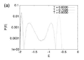
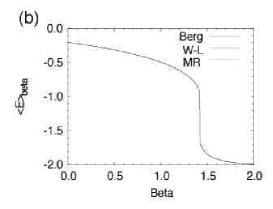
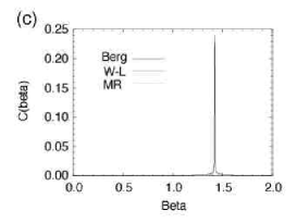
Figure 1: (a) Probability distributions of energy of 2-dimensional 10-state Potts model at three temperatures: $T=0.6000$, 0.7026, and 0.8000, and (b) average energy and (c) specific heat as functions of inverse temperature $\beta=1/T$. The results were obtained from a multicanonical MC simulation. For (b) and (c), the results from three methods of multicanonical weight factor determination are superimposed. Berg stands for Berg’s method MUCAW , W-L for Wang-Landau’s method Landau and MR for MUCAREM SO3

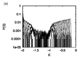
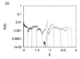
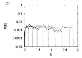
Figure 2: Probability distributions of energy for the 2-dimensional 10-state Potts model: (a) the results of REM simulation with 32 replicas and (b) and (c) iterations of MUCAREM simulations with 8 replicas.

III Results

We now present the results of our simulations based on the algorithms described in the previous section.

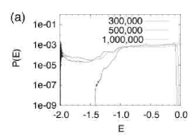
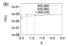
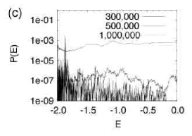
Figure 3: Probability distribution of energy during the iterative process of multicanonical weight factor determination for the 2-dimensional 10-state Potts model. The results after 300,000 MC sweeps, 500,000 MC sweeps, and 1,000,000 MC sweeps are superimposed. (a) MUCAREM SO3 , (b) Berg’s method MUCAW , and (c) Wang-Landau’s method Landau .

The first example is a spin system. We studied the 2-dimensional 10-state Potts model NSMO . The lattice size was $34\times 34$. This system exhibits a first-order phase transition Bax . In Fig. 1 we show the probability distributions of energy at three tempeartures (above the critical temperature $T_{C}$, at $T_{C}$, and below $T_{C}$) and average energy and specific heat as functions of inverse temperature. All these results imply that the system indeed undergoes a first-order phase transition.

Iterations of MUCAREM (and REMUCA) can be used to obtain an optimal MUCA weight factor MSO03 . In Fig. 2 we show the results of our MUCA weight factor determination by MUCAREM. We first made a REM simulation of 10,000 MC sweeps (for each replica) with 32 replicas (Fig. 2(a)). Using the obtained energy distributions, we determined the (preliminary) MUCA weight factor, or the density of states, by the multiple-histogram reweighting techniques of Eqs. (9) and (10). Because the trials of replica exchange are not accepted near the critical temperature for first-order phase transitions, the probability distributions in Fig. 2(a) for the energy range from $\sim-1.5$ to $\sim-1.0$ fails to have sufficient overlap, which is required for successful application of REM. This means that the MUCA weight factor in this energy range thus determined is of “poor quality.” With this MUCA weight factor, however, we made iterations of three MUCAREM simulations of 10,000 MC sweeps (for each replica) with 8 replicas (Fig. 2(b) for the first iteration and Fig. 2(c) for the third iteration). In Fig. 2(b) we see that the distributions are not completely flat, reflecting the poor quality in the phase-transition region. This problem is rapidly rectified as iterations continue, and the distributions are completely flat in Fig. 2(c), which gives an optimal MUCA weight factor in the entire energy range by the multiple-histogram reweighting techniques.

Besides MUCAREM the methods of Berg MUCAW and Wang-Landau Landau are also effective for the determination of the MUCA weight factor (or the density of states). In Fig. 3 we compare how fast these three methods converge to yield an optimal MUCA weight factor, or a flat distribution. Each figure shows three curves superimposed that correspond to the (hot-start) MUCA simulation with the weight factor that was “frozen” after 300,000 MC seeps, 500,000 MC sweeps, and 1,000,000 MC sweeps of iterations of the weight factor determination. While the results of MUCAREM and Berg’s method are similar, those of Wang-Landau method have quite different behavior. After 300,000 MC sweeps, MUCAREM and Berg’s method gives reasonably flat distribution for $E>-1.0$ and $E>-1.3$, respectively, whereas Wang-Landau method gives a distribution that is quite spiky (but already covers low-energy regions). After 500,000 MC sweeps, MUCAREM essentially gives a flat distribution in the entire energy range and Berg’s method for $E>-1.7$, while Wang-Landau method also covers the entire range (though still very rugged). After 1,000,000 MC sweeps, the three methods all give reasonably flat distributions. Details will be published elsewhere NSMO .

We now present the results of our multibaric-multithermal simulation. We considered a Lennard-Jones 12-6 potential system. We used 500 particles ($N=500$) in a cubic unit cell with periodic boundary conditions. The length and the energy are scaled in units of the Lennard-Jones diameter $\sigma$ and the minimum value of the potential $\epsilon$, respectively. We use an asterisk ($*$) for the reduced quantities such as the reduced length $r^{*}=r/\sigma$, the reduced temperature $T^{*}=k_{\rm B}T/\epsilon$, the reduced pressure $P^{*}=P\sigma^{3}/\epsilon$, and the reduced number density $\rho^{*}=\rho\sigma^{3}$ ($\rho\equiv N/V$).

We started the iterations of the multibaric-multithermal weight factor determination from a regular isobaric-isothermal simulation at $T_{0}^{*}=2.0$ and $P_{0}^{*}=3.0$. In one MC sweep we made the trial moves of all particle coordinates and the volume ($N+1$ trial moves altogether). For each trial move the Metropolis evaluation of Eq. (15) was made. Each iteration of the weight factor determination consisted of 100,000 MC sweeps. In the present case, it was required to make 12 iterations to get an optimal weight factor $W_{\rm mbt}(E,V)$. We then performed a long multibaric-multithermal MC simulaton of 400,000 MC sweeps with this $W_{\rm mbt}(E,V)$.

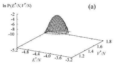
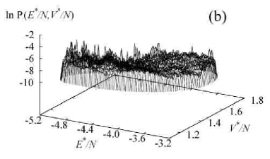
Figure 4: (a) The probability distribution ${\rm P}_{NPT}(E^{*}/N,V^{*}/N)$ in the isobaric-isothermal simulation at $(T^{*},P^{*})=(T_{0}^{*},P_{0}^{*})=(2.0,3.0)$ and (b) the probability distribution ${\rm P_{\rm mbt}}(E^{*}/N,V^{*}/N)$ in the multibaric-multithermal simulation.

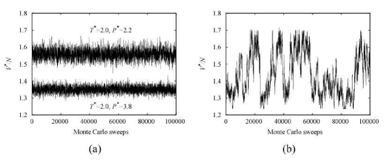
Figure 5: The time series of $V^{*}/N$ from (a) the conventional isobaric-isothermal MC simulations at $(T^{*},P^{*})=(2.0,2.2)$ and at $(T^{*},P^{*})=(2.0,3.8)$ and (b) the multibaric-multithermal MC simulation.

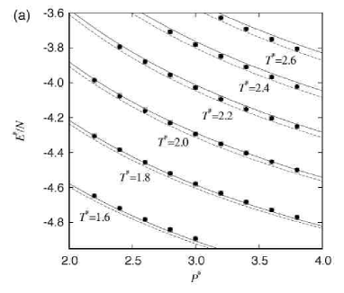
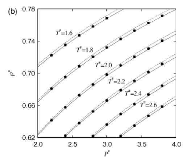
Figure 6: (a) Average potential energy per particle $<E^{*}/N>_{NPT}$ and (b) average density $<\rho^{*}>_{NPT}$ at various temperature and pressure values. Filled circles: Multibaric-multithermal MC simulations. Open squares: Conventional isobaric-isothermal MC simulations. Solid line: Equation of states calculated by Johnson et al. jzg93 . Broken line: Equation of states calculated by Sun and Teja sj93 .

Figure 4 shows the probability distributions of $E^{*}/N$ and $V^{*}/N$. Figure 4(a) is the probability distribution ${\rm P}_{NPT}(E^{*}/N,V^{*}/N)$ from the isobaric-isothermal simulation first carried out in the process (i.e., $T_{0}^{*}=2.0$ and $P_{0}^{*}=3.0$). It is a bell-shaped distribution. On the other hand, Fig. 4(b) is the probability distribution ${\rm P_{\rm mbt}}(E^{*}/N,V^{*}/N)$ from the multibaric-multithermal simulation finally performed. It shows a flat distribution, and the multibaric-multithermal MC simulation indeed sampled the configurational space in wider ranges of energy and volume than the conventional isobaric-isothermal MC simulation.

Figure 5 shows the time series of $V^{*}/N$. In Fig. 5(a) we show the results of the conventional isobaric-isothermal simulations at $(T^{*},P^{*})=(2.0,2.2)$ and (2.0,3.8), while in Figure 5(b) we give those of the multibaric-multithermal simulation. The volume fluctuations in the conventional isobaric-isothermal MC simulations are only in the range of $V^{*}/N=1.3\sim 1.4$ and $V^{*}/N=1.5\sim 1.6$ at $P^{*}=3.8$ and at $P^{*}=2.2$, respectively. On the other hand, the multibaric-multithermal MC simulation performs a random walk that covers even a wider volume range.

We calculated the ensemble averages of potential energy per particle, $<E^{*}/N>_{NPT}$, and density, $<\rho^{*}>_{NPT}$, at various temperature and pressure values by the reweighting techniques. They are shown in Fig. 6. The agreement between the multibaric-multithermal data and isobaric-isothermal data are excellent in both $<E^{*}/N>_{NPT}$ and $<\rho^{*}>_{NPT}$.

The important point is that we can obtain any desired isobaric-isothermal distribution in wide temperature and pressure ranges ($T^{*}=1.6\sim 2.6$, $P^{*}=2.2\sim 3.8$) from a single simulation run by the multibaric-multithermal MC algorithm. This is an outstanding advantage over the conventional isobaric-isothermal MC algorithm, in which simulations have to be carried out separately at each temperature and pressure, because the reweighting techniques based on the isobaric-isothermal simulations can give correct results only for narrow ranges of temperature and pressure values.

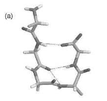
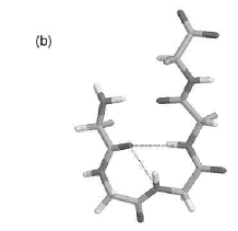
Figure 7: (a) Reference configuration 1 and (b) reference configuration 2. Only backbone structures are shown. The N-terminus is on the left-hand side and the C-terminus on the right-hand side. The dotted lines stand for hydrogen bonds. The figures were created with RasMol RasMol .

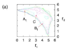
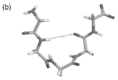
Figure 8: (a) Free-energy landscape of Met-enkephalin at $T=250$ K with respect to rms distances (Å) from the two reference configurations, $F(r_{1},r_{2})$. The labels A₁ and B₁ indicate the positions for the local-minimum states at $T=250$ K that originate from the reference configuration 1 and the reference configuration 2, respectively. The label C stands for the saddle point that corresponds to the transition state. (b) The transition state, C, between reference configurations 1 and 2. See the caption of Fig. 7 for details.

The third example is a system of a biopolymer. A brain peptide Met-enkephalin has the amino-acid sequence Tyr-Gly-Gly-Phe-Met. We fix the peptide-bond dihedral angles $\omega$ to $180^{\circ}$, which implies that the total number of variable dihedral angles is $n=19$. We neglect the solvent effects as in previous works. The low-energy configurations of Met-enkephalin in the gas phase have been classified into several groups of similar structures OKK92 ; MHO98 . Two reference configurations, called configuration 1 and configuration 2, are used in the following and depicted in Fig. 7. Configuration 1 has a $\beta$-turn structure with hydrogen bonds between Gly-2 and Met-5, and configuration 2 a $\beta$-turn with a hydrogen bond between Tyr-1 and Phe-4 MHO98 . Configuration 1 corresponds to the global-minimum-energy state and configuration 2 to the second lowest-energy state. The distance between the two configurations is $d=6.62$ and the values of the potential energy (ECEPP/2 ECEP3 ) for configuration 1 and configuration 2 are $-10.72$ kcal/mol and $-8.42$ kcal/mol, respectively.

We analyze the free-energy landscape HOO99 from the results of our multi-overlap simulation at 300 K that performs a random walk between configurations 1 and 2. We study the landscape with respect to some reaction coordinates (and hence it should be called the potential of mean force). In order to study the transition states between reference configurations 1 and 2, we first plotted the free-energy landscape with respect to the dihedral distances $d_{1}$ and $d_{2}$ of Eq. (17). However, we did not observe any transition saddle point. A satisfactory analysis of the saddle point becomes possible when the root-mean-square (rms) distance (instead of the dihedral distance) is used. Figure 8 shows contour lines of the free energy reweighted to $T=250$ K, which is close to the folding temperature (HMO97 ; BNO03 ). Here, the free energy $F(r_{1},r_{2})$ is defined by

$$F(r_{1},r_{2})=-k_{B}T\ln P(r_{1},r_{2})~{},$$ (20)

where $r_{1}$ and $r_{2}$ are the rms distances from the reference configuration 1 and the reference configuration 2, respectively, and $P(r_{1},r_{2})$ is the (reweighted) probability at $T=250$ K to find the peptide with values $r_{1},r_{2}$. The probability was calculated from the two-dimensional histogram of bin size 0.06 Å$\times$ 0.06 Å. The contour lines were plotted every $2k_{B}T$ ($=0.99$ kcal/mol for $T=250$ K).

Table 1: Free energy, internal energy, entropy multiplied by temperature at $T=250$ K (all in kcal/mol) at the two local-minimum states (A₁ and B₁) and the transition state (C) in Fig. 8(a). The rms distances, $r_{1}$ and $r_{2}$, are in Å.

Coordinate $(r_{1},r_{2})$	$F$	$U$	$-TS$
A1 (1.23, 4.83)	0	$-5.4$	5.4
B1 (4.17, 2.43)	1.0	$-3.5$	4.5
C (3.09, 4.05)	2.2	$-0.8$	3.0

Note that the reference configurations 1 and 2, which are respectively located at $(r_{1},r_{2})=(0,4.95)$ and $(4.95,0)$, are not local minima in free energy at the finite temperature ($T=250$ K) because of the entropy contributions. The corresponding local-minimum states at A₁ and B₁ still have the characteristics of the reference configurations in that they have backbone hydrogen bonds between Gly-2 and Met-5 and between Tyr-1 and Phe-4, respectively.

The transition state C in Fig. 8(a) should have intermediate structure between configurations 1 and 2. In Fig. 8(b) we show a typical backbone structure of this transition state. We see the backbone hydrogen bond between Gly-2 and Phe-4. This is precisely the expected intermediate structure between configurations 1 and 2, because going from configuration 1 to configuration 2 we can follow the backbone hydrogen-bond rearrangements: The hydrogen bond between Gly-2 and Met-5 of configuration 1 is broken, Gly-2 forms a hydrogen bond with Phe-4 (the transition state), this new hydrogen bond is broken, and finally Phe-4 forms a hydrogen bond with Tyr-1 (configuration 2).

In Ref. MHO98 the low-energy conformations of Met-enkephalin were studied in detail and they were classified into several groups of similar structures based on the pattern of backbone hydorgen bonds. It was found there that below $T=300$ K there are two dominant groups, which correspond to configurations 1 and 2 in the present article. Although much less conspicuous, the third most populated structure is indeed the group that is identified to be the transition state in the present work.

In table 1 we list the numerical values of the free energy, internal energy, and entropy multiplied by temperature at the two local-minimum states (A₁ and B₁ in Fig. 8(a)) and the transition state (C in Fig. 8(a)). Here, the internal energy $U$ is defined by the (reweighted) average ECEPP/2 ECEP3 potential energy:

$$U(r_{1},r_{2})=<E(r_{1},r_{2})>_{T}~{}.$$ (21)

The entropy $S$ was then calculated by

$$S(r_{1},r_{2})=\frac{1}{T}\left[U(r_{1},r_{2})-F(r_{1},r_{2})\right]~{}.$$ (22)

The free energy was normalized so that the value at A₁ is zero.

The state A₁ can be considered to be “deformed” configuration 1, and B₁ deformed configuration 2 due to the entropy effects, whereas C is the transition state between A₁ and B₁. Among these three points, the free energy $F$ and the internal energy $U$ are the lowest at A₁, while the entropy contribution $-TS$ is the lowest at C. The free energy difference $\Delta F$, internal energy difference $\Delta U$, and entropy contribution difference $-T\Delta S$ are 1.0 kcal/mol, 1.9 kcal/mol, and $-0.9$ kcal/mol between B₁ and A₁, 2.2 kcal/mol, 4.6 kcal/mol, and $-2.4$ kcal/mol between C and A₁, and 1.2 kcal/mol, 2.7 kcal/mol, and $-1.5$ kcal/mol between C and B₁. Hence, the internal energy contribution and the entropy contribution to free energy are opposite in sign and the magnitude of the former is roughly twice as that of the latter at this temperature.

IV Conclusions

In this article we have described the formulations of the two well-known generalized-ensemble algorithms, namely, multicanonical algorithm (MUCA) and replica-exchange method (REM). We then introduced four new generalized-ensemble algorithms as further extensions of the above two methods, which we refer to as replica-exchange multicanonical algorithm (REMUCA), multicanonical replica-exchange method (MUCAREM), multibaric-multithermal algorithm, and multi-overlap algorithm.

With these new methods available, we believe that we now have working simulation algorithms for spin systems and biomolecular systems.

Acknowledgments
This work is supported, in part, by NAREGI Nanoscience Project, Ministry of Education, Culture, Sports, Science and Technology, Japan.

References

- (1) U.H.E. Hansmann and Y. Okamoto, in Annual Reviews of Computational Physics VI, D. Stauffer (Ed.) (World Scientific, Singapore, 1999) pp. 129–157.
- (2) A. Mitsutake, Y. Sugita, and Y. Okamoto, Biopolymers (Peptide Science) 60, 96–123 (2001).
- (3) Y. Sugita and Y. Okamoto, in Lecture Notes in Computational Science and Engineering, T. Schlick and H.H Gan (Eds.) (Springer-Verlag, Berlin, 2002) pp. 304–332; cond-mat/0102296.
- (4) A.M. Ferrenberg and R.H. Swendsen, Phys. Rev. Lett. 61, 2635–2638 (1988); ibid. 63, 1658 (1989).
- (5) A.M. Ferrenberg and R.H. Swendsen, Phys. Rev. Lett. 63, 1195–1198 (1989); S. Kumar, D. Bouzida, R.H. Swendsen, P.A. Kollman, J.M. Rosenberg, J. Comput. Chem. 13, 1011–1021 (1992).
- (6) B.A. Berg and T. Neuhaus, Phys. Lett. B267, 249–253 (1991); Phys. Rev. Lett. 68, 9–12 (1992).
- (7) J. Lee, Phys. Rev. Lett. 71, 211–214 (1993); ibid. 71, 2353.
- (8) M. Mezei, J. Comput. Phys. 68, 237–248 (1987).
- (9) C. Bartels and M. Karplus, J. Phys. Chem. B 102, 865–880 (1998).
- (10) F. Wang and D.P. Landau, Phys. Rev. Lett. 86, 2050–2053 (2001).
- (11) N. Rathore and J.J. de Pablo, J. Chem. Phys. 116, 7225–7230 (2002); Q. Yan, R. Faller, and J.J. de Pablo, J. Chem. Phys. 116, 8745–8749 (2002).
- (12) U.H.E. Hansmann and Y. Okamoto, J. Comput. Chem. 14, 1333–1338 (1993). 5J. Chem. Phys. 5103 (1995) 10298.
- (13) K. Hukushima and K. Nemoto, J. Phys. Soc. Jpn. 65, 1604–1608 (1996); K. Hukushima, H. Takayama, and K. Nemoto, Int. J. Mod. Phys. C 7, 337–344 (1996).
- (14) C.J. Geyer, C.J. in Computing Science and Statistics: Proc. 23rd Symp. on the Interface, E.M. Keramidas (Ed.) (Interface Foundation, Fairfax Station, 1991) pp. 156–163.
- (15) R.H. Swendsen and J.-S. Wang, (1986) Phys. Rev. Lett. 57, 2607–2609 (1986).
- (16) K. Kimura and K. Taki, in Proc. 13th IMACS World Cong. on Computation and Appl. Math. (IMACS ’91), R. Vichnevetsky and J.J.H. Miller (Eds.), vol. 2, pp. 827–828 (1991).
- (17) D.D. Frantz, D.L. Freeman, and J.D. Doll, J. Chem. Phys. 93, 2769–2784 (1990).
- (18) M.C. Tesi, E.J.J. van Rensburg, E. Orlandini, S.G. Whittington, J. Stat. Phys. 82, 155–181 (1996).
- (19) E. Marinari, G. Parisi, J.J. Ruiz-Lorenzo, in Spin Glasses and Random Fields, A.P. Young (Ed.) (World Scientific, Singapore, 1998) pp. 59–98.
- (20) Y. Iba, Int. J. Mod. Phys. C 12, 623–656 (2001).
- (21) U.H.E. Hansmann, Chem. Phys. Lett. 281, 140–150 (1997).
- (22) Y. Sugita and Y. Okamoto, Chem. Phys. Lett. 314, 141–151 (1999).
- (23) A. Irbäck and E. Sandelin, J. Chem. Phys. 110, 12256–12262 (1999).
- (24) M.G. Wu and M.W. Deem, J. Chem. Phys. 111, 6625–6632 (1999).
- (25) D. Gront, A. Kolinski, and J. Skolnick, J. Chem. Phys. 113, 5065–5071 (2000).
- (26) A.E. Garcia and K.Y. Sanbonmatsu, Proteins 42, 345–354 (2001).
- (27) R.H. Zhou and B.J. Berne, Proc. Natl. Acad. Sci. U.S.A. 99, 12777–12782 (2002).
- (28) Y. Sugita, A. Kitao, and Y. Okamoto, J. Chem. Phys. 113, 6042–6051 (2000).
- (29) Y. Sugita and Y. Okamoto, Chem. Phys. Lett. 329, 261–270 (2000).
- (30) A. Mitsutake and Y. Okamoto, Chem. Phys. Lett. 332, 131–138 (2000).
- (31) A. Mitsutake, Y. Sugita, and Y. Okamoto, J. Chem. Phys. 118, 6664–6675 (2003); ibid. 118, 6676–6688 (2003).
- (32) H. Okumura and Y. Okamoto, submitted for publication; cond-mat/0306144.
- (33) B.A. Berg, H. Noguchi, and Y. Okamoto, Phys. Rev. E, in press; cond-mat/0305055.
- (34) N. Metropolis, A.W. Rosenbluth, M.N., Rosenbluth, A.H. Teller, Teller, E. (1953) J. Chem. Phys. 21, 1087–1092.
- (35) I.R. McDonald, Mol. Phys. 23, 41 (1972).
- (36) U.H.E. Hansmann, M. Masuya, and Y. Okamoto, Proc. Natl. Acad. Sci. U.S.A. 97, 10652–10656 (1997).
- (37) T. Nagasima, Y. Sugita, A. Mitsutake, and Y. Okamoto, in preparation.
- (38) R.J. Baxter, J. Phys. C 6, L445 (1973).
- (39) B.A. Berg, Nucl. Phys. B (Proc. Suppl.) 63A-C, 982–984 (1998).
- (40) J.K. Johnson, J.A. Zollweg, and K.E. Gubbins, Mol. Phys. 78, 591 (1993).
- (41) T. Sun and A.S. Teja, J. Phys. Chem. 100, 17365 (1996).
- (42) Y. Okamoto, K. Kikuchi, and H. Kawai, Chem. Lett. 1992, 1275–1278 (1992);
- (43) A. Mitsutake, U.H.E. Hansmann, and Y. Okamoto, J. Mol. Graphics Mod. 16, 226–238; 262–263 (1998);
- (44) M.J. Sippl, G. Némethy, and H.A. Scheraga, J. Phys. Chem. 88, 6231–6233 (1984), and references therein.
- (45) U.H.E. Hansmann, Y. Okamoto, and J.N. Onuchic, Proteins 34, 472–483 (1999).
- (46) R.A. Sayle and E.J. Milner-White, Trends Biochem. Sci. 20, 374–376 (1995).