Optical detection of fractional particle number in an atomic Fermi-Dirac gas

Abstract

We study theoretically a Fermi-Dirac atomic gas in a one-dimensional optical lattice coupled to a coherent electromagnetic field with a topologically nontrivial soliton phase profile. We argue that the resulting fractional eigenvalues of the particle number operator can be detected via light scattering. This could be a truly quantum mechanical measurement of the particle number fractionalization in a dilute atomic gas.

It has been known for a while that, in the presence of a topologically nontrivial bosonic background field, fermionic particles may carry a fractional part of an elementary quantum number JAC76 ; NIE86 . In the condensed matter regime this phenomenon was introduced SU79 to describe conjugated polymers. The existence of fractionally charged excitations in the polymers is typically demonstrated indirectly by detecting the reversed spin-charge relation HEE88 . The fractional quantum Hall effect (FQHE) can also be explained by invoking quasiparticles, each with a fraction of an electron’s charge laughlin . The fluctuations of the tunneling current in low-temperature FQHE regime have been measured DEP97 . Interpreting the current shot noise according to the Johnson-Nyquist formula duly suggests that the current is carried by the fractional Laughlin quasiparticles. Analogous experiments have determined the fractional expectation value of the charge in FQHE in the Coulomb blockade regime GOL95 .

We have earlier proposed a system of Fermi-Dirac (FD) atoms in an optical lattice that should display fractional atom numbers RUO02 . In the present Letter we argue that usual optical methods such as phase contrast imaging and measurements of the intensity of light scattered by the atoms extract information about the fractional fermion number. The technical challenges are severe, but in principle both the expectation value and the fluctuations of the atom number are accessible to experiments.

Briefly, we consider a FD atom OLS98 with a $\Lambda$ scheme for two active states (say, Zeeman states in different hyperfine levels) that can be coupled by one or two-photon electromagnetic (em) transitions RUO02 . The atoms reside in a 1D optical lattice lattices that holds the two states at alternating sites $\lambda/4$ apart, where $\lambda$ denotes the wavelength of lattice light. By making use of the em transitions, we assume, it is possible to make the atoms hop between the adjacent sites so that they at the same time change their internal state. The lattice Hamiltonian is

$${H\over\hbar}=\sum_{k}\left[\delta_{k}c^{\dagger}_{k}c_{k}+\kappa_{k}(c^{\dagger}_{k+1}c_{k}+c^{\dagger}_{k}c_{k+1})\right]\,.$$ (1)

Here $c_{k}$ is the annihilation operator for the fermionic atoms at site $k$, $\hbar\delta_{k}$ is the energy of the atoms at $k$, and $\kappa_{k}$ are the are hopping matrix elements tailored to suit our purposes. The literature is replete with studies of similar systems BEL83 ; KIV ; GW , but our treatment is unusual in that we never resort to the continuum limit.

It is easy to see that the matrix $U_{kp}$ whose columns are the orthonormal eigenvectors of the eigenvalue problem

$$(\delta_{k}-\omega)a_{k}+\kappa_{k}a_{k+1}+\kappa_{k-1}a_{k-1}=0$$ (2)

may be employed to diagonalize the Hamiltonian (1). In terms of the new fermion operators $\gamma_{p}\equiv\sum_{k}U_{kp}c_{k}$, we have $H/\hbar=\sum_{p}\omega_{p}\gamma^{\dagger}_{p}\gamma_{p}$ . Without a loss of generality, the couplings $\kappa_{k}$ are assumed real, and so we take $U$ real and orthogonal; $U_{kp}^{-1}=U_{pk}$. In this paper all calculations are done directly numerically.

Even though the optical lattice may be part of a larger trap and the wider trap could generate interesting physics in its own right, we simplify by putting $\delta_{k}=0$. The fractional charge arises from certain types of defects in the couplings $\kappa_{k}$. We illustrate by assuming a dimerized lattice generated by the coupling matrix element that alternates from site to site between two values $a+\mu$ and $a-\mu$, except that at the center of the lattice there is a defect such that the same coupling matrix element appears twice. We take the number of lattice sites to be $N_{s}\equiv 2N_{h}+1\equiv 4n+1$, where $n$ is an integer itself, and number the sites with integers ranging from $-N_{h}$ to $N_{h}$. For illustration, pick $n=2$, use an x to denote a lattice site, and $\pm$ the couplings $a\pm\mu$, then our lattice with the couplings reads

$${\rm x}+{\rm x}-{\rm x}+{\rm x}-{\rm x}-{\rm x}+{\rm x}-{\rm x}+{\rm x}\,$$ (3)

It is then easy to see from the structure of Eq. (2) that if $\omega$ is an eigenvalue, then so is $-\omega$; and the eigenvectors transform into one another by inverting the sign of every second component. We will label the eigenvectors as $-N_{h}\ldots N_{h}$ in ascending order of frequency, and assign the labels $\pm p$ to such $\pm$ pair of states. Correspondingly, the transformation matrix $U$ satisfies $|U_{kp}|=|U_{k,-p}|$.

But under our assumptions, the number of eigenvalues and eigenstates is odd. The $\pm$ symmetry implies that an odd number of the eigenvalues must equal zero. Except for special values of the couplings $a$ and $\mu$, there is one zero eigenvalue. We call the corresponding eigenstate the zero state. Provided $a$ and $\mu$ have the same sign and $|a|>|\mu|$, all odd components in the zero state equal zero and the even components are of the form

$$x_{k}=x_{0}\left({-\displaystyle{a-\mu\over a+\mu}}\right)^{|k|/2}\,.$$ (4)

The zero state becomes the narrower, the closer in absolute value $a$ and $\mu$ are.

The dimerized optical lattice resulting from the alternating pattern of the hopping matrix elements causes the single-particle density of states to acquire an energy gap, which in the limit $N_{s}\rightarrow\infty$ equals $4\hbar|\mu|$ . The zero state is located at the center of the gap. The resulting excitations at half the gap energy could be detected by resonance spectroscopy. This provides indirect evidence of fractionalization, as in the polymer systems HEE88 . Because in our scheme RUO02 the gap is proportional to the amplitude of the em field inducing the hopping, the size of the energy gap can be controlled experimentally. The effective zero temperature limit, $|\mu|\gg k_{B}T/\hbar$, might then be reached under a variety of experimental conditions.

Suppose next that the system is at zero temperature, and contains $N_{f}=N_{h}+1$ fermions. The exact eigenstates $p$ are then filled up to zero state and empty at higher energies, with occupation numbers $n_{p}$ = 0 or 1. The number operator for the fermions at site $k$ correspondingly reads $c^{\dagger}_{k}c_{k}=\sum_{pq}U_{kp}U_{kq}\gamma^{\dagger}_{p}\gamma_{q}$, so the expectation value of the fermion number at the site $k$ is

$$\langle c^{\dagger}_{k}c_{k}\rangle = \sum_{p=-N_{h}}^{0}|U_{kp}|^{2}=\hbox{$1\over 2$}\sum_{p=-N_{h}}^{N_{h}}|U_{kp}|^{2}+\hbox{$1\over 2$}|U_{k0}|^{2}$$ (5)

$$= \hbox{$1\over 2$}+\hbox{$1\over 2$}|U_{k0}|^{2}\,.$$

The second equality is based on the symmetry $|U_{kp}|=|U_{k,-p}|$, and the third on the orthogonality of the matrix $U$. By virtue of the same orthogonality, localized with the zero state there is a lump with $\hbox{$1\over 2$}\sum_{k}|U_{k0}|^{2}=\hbox{$1\over 2$}$ fermions on top of a uniform background of half a fermion per site. This lump is the celebrated half of a fermion. So far we only deal with the expectation values of the atom numbers, but we will demonstrate shortly that the fluctuations in atom number can be small as well.

Fractionilization is a more robust phenomenon than our discussion may let on. Something akin to a localized zero state occurs as soon as the regular alternation of the couplings between adjacent states gets out of rhythm around a defect. In particular, the defect does not have to be confined to one lattice site, which might make the experiments easier. The half-fermion is localized, so it does not critically depend on the number or parity of sites, and not even on the exact number of the fermions. We will enumerate such variations of the theme elsewhere.

We next turn to the optical detection of the FD gas. We assume that far off-resonant light excites the atoms, whereupon the 1D optical lattice may be considered optically thin. We take the sources residing at each site to be much smaller than the wavelength of light. Then the (positive frequency part of the) field operator for scattered light is JAV95 $\hat{E}^{+}=C\sum_{k}\alpha_{k}c^{\dagger}_{k}c_{k}$, where $C$ is a constant containing the overall intensity scale of the driving light. Henceforth we scale so that $C=1$. The factors $\alpha_{k}$ include aspects such as intensity and phase profile of the driving light, effects of the spin state at each site $k$ on the light-atom coupling, and propagation phases of light from the lattice site to the point of observation.

In forward scattering and variations thereof such as phase contrast imaging, the scattered and the incoming light interfere. The ultimate measurement of the intensity in effect records the expectation value of the electric field $E=\langle\hat{E}^{+}\rangle$. The observable at the detector is

$$E=\sum_{k}\alpha_{k}\langle c^{\dagger}_{k}c_{k}\rangle=\sum_{kp}\alpha_{k}U^{2}_{kp}n_{p}\,.$$ (6)

This is a linear combination of the expectation values of the numbers of fermions at each lattice site with the coefficients $\alpha_{k}$, which are to some extent under the control of the experimenter. In the absence of interference with the incoming light, the simplest observable is light intensity $I=\langle\hat{E}^{-}\hat{E}^{+}\rangle$. The detector then probes the quantity characteristic of the FD statistic

$$I = \sum_{kl}\alpha^{*}_{k}\alpha_{l}\langle c^{\dagger}_{k}c_{k}c^{\dagger}_{l}c_{l}\rangle=|E|^{2}+\Delta I\,;$$ (7)

$$\Delta I = \sum_{klpq}\alpha^{*}_{k}\alpha_{l}U_{kp}U_{kq}U_{lp}U_{lq}n_{p}(1-n_{q})\,.$$ (8)

We now construct a numerical example about the use of forward scattering to detect the fractional particle. We make use of the fact that the fermion species at the alternating lattice sites are likely to be different. We assume that a given driving light is far above resonance with the fluorescing transition in one species and far below resonance in the other, and that the matrix elements for dipole transitions are comparable. It is then possible to find a tuning of the laser such that the intensity of scattered light is the same for both species. Moreover, the light scattered by the two species are out of phase by $\pi$, and out of phase with the incident light by $\pi/2$. With the usual tricks of phase contrast imaging, the relative phase of incident and scattered light is then adjusted so that that in interference light from one species directly adds to the incident light, and light from the other species subtracts.

The second element of the argument is a rudimentary model for an imaging system with a finite aperture. Let us assume the geometry has been arranged in such a way that all Fourier components of light in the plane of the aperture up to the absolute value $K$ are passed, the rest blocked. The effect on imaging from the object plane to image plane can be analyzed by taking the Fourier transform of the object, filtering with the multiplier $\theta(K-|{\bf k}_{\perp}|)$, and transforming back. The filtered image of the lattice filtered is then proportional to

$$E({\bf r})=\sum_{k}(-1)^{k}\langle c^{\dagger}_{k}c_{k}\rangle\,{2J_{1}(K|{\bf r}-{\bf r}_{k}|)\over K|{\bf r}-{\bf r}_{k}|}\,.$$ (9)

We choose the parameters $\mu=0.1\,a$, and the numbers of sites and fermions $N_{s}=129$ and $N_{f}=65$. We take the numerical aperture $F=1$ for the imaging system, and the corresponding maximum possible cutoff wave number $K=2\pi/(\sqrt{5}\lambda)$. In Fig. 1 we plot the optically imaged fermion lattice along the line of the atoms (dashed line), and the number of fermionic atoms in excess of the average occupation number $1\over 2$ for the even-numbered sites that carry the zero state (solid line), as obtained from Eq. (5). The curves are normalized so that the maxima overlap. The imaging system picks up a resolution rounded version the half-fermion hump.

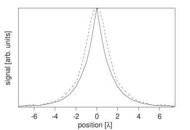
Figure 1: Optical image (dashed line) of a zero state carrying half of a fermion (solid line) for a specific imaging system as discussed in the text. The size of the soliton is set by the choices $N_{s}=129$, $N_{f}=65$, $\mu=0.1\,a$.

In fact, phase contrast imaging has been used for nondestructive monitoring of a Bose-Einstein condensate AND96 , and the absorption of a single trapped ion has been detected experimentally ION80 . While a lot of assumptions went into our specific example, an experiment along these lines should be feasible with the technology available today.

With illumination of the optical lattice by a focused light beam and detection of scattered intensity in a direction of constructive interference, it is in principle also possible to realize a situation in which the weights approximately make a Gaussian distribution around the zero state, $\alpha_{k}=e^{-(k/w)^{2}}$. In such a case the observable $\hat{N}=\hat{E}^{+}$ is just a linear combination of the occupation numbers of the lattice sites, the quantity $E$ is the expectation value thereof, and $\Delta I$ is nothing but the squared fluctuations of $\hat{N}$, $\Delta I=(\Delta N)^{2}=\langle{\hat{N}}^{2}\rangle-\langle{\hat{N}}\rangle^{2}$.

To illustrate, we take a lattice with $N_{s}=1025$ sites, pick the parameters $\mu=0.1\,a$, put in $N_{f}=513$ fermions so that the zero state is the last filled stated, and find the rms fluctuation of the fermion number $\Delta N$ as a function of the width of the weight function $w$. The result is shown in Fig. 2 on a log-log plot. The notch around $w=1$ indicates that at this point the weight factors $\alpha_{k}$ start to cover several lattice sites. Another break in the curve is seen at about $w=10$, when the weight function covers the whole zero state. Thereafter the fluctuations behave as $\Delta N\propto w^{-1/2}$. The fermion number $\hat{N}$ under the weight function becomes more sharply defined as the region for averaging grows broader. Finally, at $w$ of a few hundred, the weights $\alpha_{k}$ effectively cover the entire lattice. The fluctuations then decrease even faster with increasing $w$, as is appropriate for the fixed fermion number in the lattice as a whole.

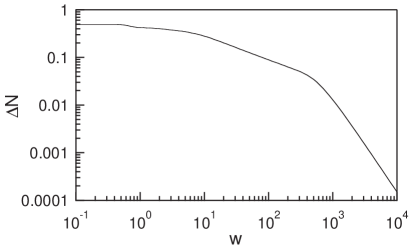
Figure 2: Fermion number fluctuations $\Delta N$ under a Gaussian envelope of width $w$, for $N_{s}=1025$, $N_{f}=65$, $\mu=0.1\,a$.

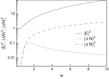
Figure 3: The intensity of light scattered from the optical lattice if the fermion numbers did not fluctuate ($|E|^{2}$), and the additional intensity due to fermion number fluctuations ($(\Delta N)^{2}$), as a function of the size of the focus $w$ of the driving light given in the lattice units of $\lambda/4$. We also display the added intensity $(\Delta N)^{2}_{i}$ that would result if fermion number fluctuations were uncorrelated between adjacent lattice sites. The soliton parameters are $N_{s}=129$, $N_{f}=65$, $\mu=0.9\,a$.

In the standard half-integer fermion number arguments one subtracts a neutralizing background of precisely $1\over 2$ charge per lattice site, whereupon $\langle\hat{N}\rangle\rightarrow\hbox{$1\over 2$}$ and $\Delta N\rightarrow 0$ with an increasing width $w$. The intermediate regime that occurs once the zero state is covered is the crux of the matter. Not only does the expectation value of fermion number equal $1\over 2$, but fluctuations are also small. After the subtraction, the fermion number has the eigenvalue $1\over 2$. From the quantum optics viewpoint, this is something of a conjuror’s trick. Correlated fluctuations in fermion number between adjacent sites create an impression of a sharp eigenvalue in a smoothly weighted sum of the occupation number operators for the lattice sites.

The scattered light carries signature of the fluctuations in the scattered intensity. We demonstrate by plotting in Fig. 3 separately the contribution $|E|^{2}$, as if the fermion numbers were precisely fixed, and the fluctuation terms $(\Delta N)^{2}$. We also show the quantity $(\Delta N)_{i}^{2}$ that remains from the fluctuation term if we only keep the contributions with $k=l$ in Eq. (8), as if the fermion number fluctuations at adjacent sites were uncorrelated. These are given as functions of the width of the focus $w$ of the laser beam. Here $N_{s}=129$, $N_{f}=65$, and we choose $\mu=0.9\,a$ to make a sharply localized zero state.

Even with a very narrow focus of the laser, $w=4$ or about one wavelength, the contribution from the fluctuations is two orders of magnitude below the coherent intensity, whereas the fluctuations from uncorrelated fermion numbers would make a contribution an order magnitude smaller than the coherent intensity. As our detection light was assumed to be far-off resonance, the photon number fluctuations are Poissonian. Under otherwise ideal conditions, the detection of about a hundred photons could therefore reveal the difference between correlated and uncorrelated fermion numbers at adjacent site, whereas a quantitative study of the actual correlated fermion numbers requires the detection of about 10,000 photons. Unfortunately, a large number of scattered photons means a large number of recoil kicks on the fermions. Currently available optical lattices likely cannot absorb the assault of hundreds of photon recoils without developing some form of a dynamics that complicates the phenomena we are analyzing. In the coherent detection of the fermion number, however, the photon recoils could be suppressed by tuning the energy gap to be much larger than the photon recoil energy.

It is instructive to note that, at the level we have discussed (amplitude or intensity measurements), optical detection of the anomalously small fermion number fluctuations responsible for fractionilization has to be coherent and rely on interference of light scattered from different lattice sites. If a too broad angular average or other such cause wipes out the interferences [$\alpha^{*}_{k}\alpha_{l}\rightarrow\delta_{kl}\alpha^{*}_{k}\alpha_{k}$], we are back to adding fermion number fluctuations from different lattice sites as if they were independent.

Although we, of course, do not aim at a specific experimental design, a few variations to potentially overcome the technical limitations we have noted bear a mention. First, we have implicitly assumed that the lattice light and the detection light have the same wavelengths. By angling the beams used to make the optical lattice, or possibly by using microlens arrays DUM02 , the optical lattice can be stretched. The resolution limit imposed by the wavelength of the detection light could be circumvented. Second, so far we have dealt with what in essence is spontaneous Bragg scattering. Recently, induced Bragg scattering has been introduced as a method to study the condensates in detail STA99 . How induced scattering works in the case of a 1D lattice under inhomogeneous illumination is not clear at the moment, but conceivably the Bragg pulses could be made so short that the harmful effects of photon recoil do not have time to build up during the measurement.

We have discussed optical detection of the half-fermion that can arise from a topological defect in an optical lattice holding a FD gas. Even though both the average fermion number and its fluctuations are in principle amenable to optical measurements, experiments will evidently have to await further development of technology. In the interim, the most valuable outcome of the kind of an analysis we have presented would probably be the insights it brings into the phenomenon of a fractional fermion number and its prospective applications.

We acknowledge financial support from the EPSRC, NSF, and NASA.

References

- (1) R. Jackiw and C. Rebbi, Phys. Rev. D 13, 3398 (1976).
- (2) A. Niemi and G. Semenoff, Phys. Reports 135, 99 (1986).
- (3) W.P. Su, J.R. Schrieffer, and A.J. Heeger, Phys. Rev. Lett. 42, 1698 (1979).
- (4) A.J. Heeger et al., Rev. Mod. Phys. 60, 781 (1988).
- (5) R. B. Laughlin, H. Störmer and D. Tsui, Rev. Mod. Phys. 71, 863 (1999).
- (6) R. de-Picciotto et al., Nature 389, 162 (1997); L. Saminadayar et al., Phys. Rev. Lett. 79, 2526 (1997).
- (7) V.J. Goldman and B. Su, Science 267, 1010 (1995).
- (8) J. Ruostekoski, G. V. Dunne, and J. Javanainen, Phys. Rev. Lett. 88, 180401 (2002).
- (9) The fractionilization could also be realized with tightly confined 1D bosonic atoms in the Tonks gas regime, where the impenetrable atoms obey FD statistics, M. Olshanii, Phys. Rev. Lett. 81, 938 (1998).
- (10) For recent experiments on bosonic atoms in optical lattices see, e.g., C. Orzel et al., Science 291, 2386 (2001); M. Greiner et al., Nature 415, 39 (2002).
- (11) J.S. Bell and R. Rajaraman, Nucl. Phys. B220, 1 (1983).
- (12) S. Kivelson and J. R. Schrieffer, Phys. Rev. B 25, 6447 (1982); R. Jackiw et al, Nucl. Phys. B225, 233 (1983).
- (13) J. Goldstone and F. Wilczek, Phys. Rev. Lett. 47, 986 (1981).
- (14) J. Javanainen and J. Ruostekoski, Phys. Rev. A 52, 3033 (1995).
- (15) M. R. Andrews et al., Science 273, 84 (1996).
- (16) D. J. Wineland, W. M. Itano and J. C. Bergquist, Opt. Lett. 12, 389 (1987).
- (17) R. Dumke et al., Phys. Rev. Lett. 89, 220402 (2002).
- (18) D.M. Stamper-Kurn et al., Phys. Rev. Lett. 83, 2876 (1999); J. Steinhauer et al., ibid. 90, 60404 (2003).