AC losses in type-II superconductors induced by nonuniform fluctuations of external magnetic field

Abstract

Magnetic field fluctuations are inevitable in practical applications of superconductors and it is often necessary to estimate the AC losses these fluctuations induce. If the fluctuation wavelength is greater than the size of a superconductor, known estimates for an alternating uniform external magnetic field can be employed. Here we consider the opposite case and analyze, using a model critical-state problem, penetration of spatially nonuniform fluctuations into type-II superconductors. Numerical simulation is based on a variational formulation of the Bean model. The analytical solutions, found in a weak penetration limit, are used to evaluate AC losses for two types of fluctuations: the running and standing waves. It is shown that for spatially nonuniform fluctuations the losses are better characterized by the fluctuation penetration depth than by the fluctuation amplitude. The results can be used to estimate the AC losses in flywheels, electric motors, magnetic shields, etc.

I Introduction

The possible range of currents and magnetic fields as well as the economic gains of implementation of type-II superconductors in power transmission lines, current leads, fault current limiters, magnetic shields, bearings, etc. are often limited by AC losses and the necessity to remove the generated heat out of the system. Thus, application of bulk high-Tc superconductors in flywheel systems and magnetic bearings is promising because of no friction between the moving parts and, hence, no energy losses by friction. However, rotating permanent magnets used in such devices always produce somewhat irregular magnetic field; moving field irregularities cause hysteretic losses and relaxation of levitation property [1].

The mathematical models, used to analyze magnetization of type-II superconductors and to evaluate AC losses, involve highly nonlinear partial differential equations that have been solved mostly for superconductors in a uniform alternating external magnetic field (see [2, 3, 4, 5, 6] and the references therein). In many practical situations, however, the external magnetic field is not exactly uniform and can be better presented as a superposition of a uniform part and spatiotemporal fluctuations with the characteristic length scale less than the size of a superconductor. The fluctuations are often stochastic but, for example, in the case of a flywheel system, are induced by rotation of permanent magnets and may be approximated by a running wave. If there are no moving parts as, e.g., in the case of magnetic shields or transformers, nonuniform magnetic field fluctuations in the form of a standing wave can, probably, serve as a better approximation.

Our aim is to study the penetration of nonuniform magnetic field fluctuations into a hard superconductor and to evaluate the accompanying AC losses. We start with a convenient for numerical simulations variational general formulation of the Bean critical-state model (section II), then consider the simplest geometric configuration, a superconductive slab placed between two parallel sheets of external current. Even in this simplest case the problem becomes nontrivial if the external current and, hence, also the external magnetic field, are nonuniform. We assume the external field fluctuations are induced by a given current in the form of either a running or a standing wave and solve, first, the magnetization problems numerically (section III). Simple physical arguments allow us to find also asymptotic analytical solutions for small fluctuations (section IV). We further extend these solutions by presenting them as the zero-order terms of consistent asymptotic expansions, find the first order corrections (appendices I and II), and, finally, determine the asymptotic AC losses for small fluctuations (section V). We analyze the dependance of the leading AC loss term on the first order correction to current density distribution.

II Variational formulation of the Bean model

Let a superconductor occupying domain $\Omega\subset\mathbb{R}^{3}$ be placed into magnetic field $\mathbf{H}_{e}(r,t)$ induced by a given external current with the density $\mathbf{J}_{e}(r,t)$ (here $r=\{x,y,z\}$ and $\mathbf{J}_{e}=0$ in $\Omega$). In accordance with the Faraday law, an alternating magnetic flux induces electric field and, hence, an eddy current inside the superconductor. In an ordinary conductor, the vectors of the electric field and current density are related by the linear Ohm law. Type-II superconductors are, instead, characterized in the Bean critical state model [7] by a highly nonlinear current-voltage relation which gives rise to a free boundary problem.

Let us assume

$$\mathbf{E}=\rho\mathbf{J}$$ (1)

and employ the usual Bean model relations determining the effective resistivity of a superconductor, $\rho(r,t)$, implicitly. Namely, the Bean model states that the effective resistivity is nonnegative,

$$\rho(r,t)\geq 0,$$ (2)

the current density cannot exceed some critical value,

$$|\mathbf{J}(r,t)|\leq J_{c},$$ (3)

and, if the current density is subcritical, the resistivity is zero:

$$|\mathbf{J}(r,t)|<J_{c}\rightarrow\rho(r,t)=0.$$ (4)

Since no current is supposed to be fed into the superconductor by an electric contact, the current density inside $\Omega$ should satisfy the zero divergence condition and have a zero normal component at the domain boundary $\partial\Omega$:

$$\nabla\cdot\mathbf{J}=0\ \mbox{in}\ \Omega,\ \ \ \ \ \ \mathbf{J}_{n}=0\ \mbox{on}\ \partial\Omega.$$ (5)

To derive a variational formulation of the magnetization problem, we define the set $K$ of possible current densities,

$$\mathbf{J}\in K=\left\{\mathbf{\Phi}(r,t)\ \left|\begin{array}[]{lr}\nabla\cdot\mathbf{\Phi}=0&\mbox{in}\ \Omega,\\ \mathbf{\Phi}_{n}=0&\mbox{on}\ \partial\Omega,\\ |\mathbf{\Phi}|\leq J_{c}&\mbox{in}\ \Omega\end{array}\right.\right\},$$

and express the electric field via the vector and scalar magnetic potentials,

$$\mathbf{E}=-\partial_{t}\mathbf{A}-\nabla\psi.$$ (6)

We further eliminate the scalar potential by multiplying (6) by $\mathbf{\Phi}-\mathbf{J}$, integrating over $\Omega$, and making use of the zero divergence condition for functions from the set $K$,

$$\left(\mathbf{E},\mathbf{\Phi}-\mathbf{J}\right)=-\left(\partial_{t}\mathbf{A},\mathbf{\Phi}-\mathbf{J}\right),$$ (7)

for $\mathbf{J},\mathbf{\Phi}\in K.$ Here $(\mathbf{u},\mathbf{v})=\int_{\Omega}\mathbf{u}\cdot\mathbf{v}\,d\Omega$ is the scalar product of two functions.

Since $\mathbf{E}$ and $\mathbf{J}$ satisfy the current-voltage relations of the Bean model, the scalar product on the left side of (7) is nonpositive for any $\mathbf{\Phi}\in K$. Indeed, using (1)-(4) we obtain:

$$\mathbf{E}\cdot\mathbf{J}=|\mathbf{E}||\mathbf{J}|=|\mathbf{E}|J_{c}\geq|\mathbf{E}||\mathbf{\Phi}|\geq\mathbf{E}\cdot\mathbf{\Phi}.$$ (8)

Up to the gradient of a scalar function, determined by the gauge and also eliminated by the scalar product with $\mathbf{\Phi}-\mathbf{J}$, the vector potential is a convolution of the Green function of Laplace equation, $G(r)=1/4\pi|r|$, and the total current density $\mathbf{J}(r,t)+\mathbf{J}_{e}(r,t)$:

$$\mathbf{A}=\mu_{0}G*(\mathbf{J}+\mathbf{J}_{e})$$

(it is assumed that the magnetic permeability of superconductor is equal to that of vacuum, $\mu_{0}$.) We arrived at the following variational formulation of the magnetization problem:

$$\begin{array}[]{c}\mbox{Find}\ \mathbf{J}\in K\ \mbox{such that}\\ \left(G*\partial_{t}\{\mathbf{J}+\mathbf{J}_{e}\},\mathbf{\Phi}-\mathbf{J}\right)\geq 0\ \ \mbox{for any}\ \mathbf{\Phi}\in K,\\ \mathbf{J}|_{t=0}=\mathbf{J}_{0}(r),\end{array}$$ (9)

where $\mathbf{J}_{0}\in K$ is a given initial distribution of the current density.

The problem (9) is an evolutionary variational inequality with a nonlocal operator and has a unique solution [8]. This inequality is written for the induced current density alone: the effective resistivity $\rho$ has been used to derive the inequality (8) and then excluded. It has been shown [8] that, in the Bean model, $\rho(r,t)$ is the Lagrange multiplier related to the current density constraint (3). Of course, the same inequality may be written as $\left(G*\partial_{t}\mathbf{J}+\frac{1}{\mu_{0}}\partial_{t}\mathbf{A}_{e},\mathbf{\Phi}-\mathbf{J}\right)\geq 0$ for any $\mathbf{\Phi}\in K$, where $\mathbf{A}_{e}$ is the external vector potential; such formulation can be more convenient in some cases.

We note that, although the variational formulations where the solution is sought as an extremal point of some functional are much more familiar, the variational inequalities do appear in many problems of mechanics and physics containing a unilateral constraint or a non-smooth constitutive relation (see [9]). The methods for numerical solution of variational inequalities are well developed [10]. Nevertheless, solution of (9) in the general 3d case is certainly a challenging problem not only because of huge number of finite elements needed: the nonlocal operator of convolution leads to a dense matrix of the discretized problem, and the zero divergence condition (5) is not so easy to account for numerically, although the edge finite elements and tree-cotree decomposition can be helpful (see [11, 12]). Similar difficulties are typical also of other formulations of the magnetization problem [13, 2]. That is why the magnetization problems were solved mainly for one and two-dimensional configurations. Below, we use a model 2d problem to simulate the penetration of nonuniform magnetic field fluctuations into a hard superconductor numerically and to calculate the AC losses asymptotically for weak penetration.

III Two types of field fluctuations

To simulate the penetration of magnetic field fluctuations into a superconductor, let us consider the simplest possible configuration: a superconductive slab $-l\leq x\leq l$ placed between two sheets of external current at $x=\pm a$, $a>l$ (Fig. 1).We assume the external current is parallel to $z$-axis, $\mathbf{J}_{e}=J_{e}{\mathbf{e}}_{z}$.

Figure 1: Infinite slab between two parallel sheets of current.

Having in mind, e.g., a superconductor moving along the axis of a solenoid with slightly nonuniform winding, we present the external current $J_{e}$ as a sum of its uniform component $I_{e}$ and a wave moving along the $y$-axis with the velocity $v$:

$$J_{e}=\left[I_{e}+i_{e}\sin\{k(y-vt)\}\right][\delta(x+a)-\delta(x-a)].$$ (10)

We will also consider the standing wave of magnetic field induced by the current

$$J_{e}=\left[I_{e}+i_{e}\sin(ky)\sin(2\pi ft)\right][\delta(x+a)-\delta(x-a)].$$ (11)

If the sheet current density were uniform, the Bean model equations for slab magnetization could be solved easily. It is more difficult to analyze the magnetization in a nonuniform magnetic field induced by the external currents (10) or (11), and we will use a 2d reformulation of the variational inequality (9) and the numerical method proposed in [4] for cylinders of arbitrary cross sections in a perpendicular magnetic field. The method can be employed for any distribution of external currents. Taking the cylinder cross section to be a rectangle, $-l\leq x\leq l,\ L\leq y\leq L$, we model the development near the slab surfaces of critical current zones that shield the fluctuating component of external magnetic field.

The shielding current inside the superconductor is directed along the $z$-axis and does not depend on $z$, $\mathbf{J}=J(x,y,t)\mathbf{e}_{z}$, so the conditions (5) are satisfied automatically. We may redefine $\Omega$ to be the cylinder cross section and solve a 2d problem in this domain. One should, however, be cautious: the eddy current running in the positive $z$-axis direction has to return back (no transport current is applied; see [4] for solution of problems with transport current). As a trace of the 3d zero-divergence conditions (5), the condition

$$\int_{\Omega}J(x,y,t)\,d\Omega=0$$

has to be satisfied for all $t$. The set of admissible (scalar) current densities becomes

$$K=\left\{\Phi(x,y,t)\ \left|\ |\Phi|\leq J_{c}\ \mbox{in}\ \Omega,\ \ \int_{\Omega}\Phi\,d\Omega=0\right.\right\}.$$

The variational inequality (9) can also be rewritten for scalar current densities,

$$\begin{array}[]{c}\mbox{Find}\ {J}\in K\ \mbox{such that}\\ \left(G*\partial_{t}\{{J}+{J}_{e}\},{\Phi}-{J}\right)\geq 0\ \ \mbox{for any}\ {\Phi}\in K,\\ {J}|_{t=0}={J}_{0}(r),\end{array}$$ (12)

where $G(r)=-\frac{1}{2\pi}\ln|r|$ is now the Green function of Laplace equation in $\mathbb{R}^{2}$ and $r=\{x,y\}$.

To solve the problem numerically, we use first the finite difference discretization in time and obtain, for each time layer, the stationary variational inequalities

$$\mbox{Find}\ {J}\in K\ \mbox{such that}\ \ (G*\{J+J_{e}-\widehat{J}-\widehat{J}_{e}\},\Phi-J)\geq 0\ \ \mbox{for any}\ \Phi\in K,$$

where $\widehat{J},\widehat{J}_{e}$ are the values from the previous time layer. It can be shown that these variational inequalities are equivalent to the optimization problems

$$\begin{array}[]{cc}\min&\frac{1}{2}(G*J,J)+(g,J),\\ J\in K&\end{array}$$ (13)

where $g=G*\{J_{e}-\widehat{J}-\widehat{J}_{e}\}$. The convolution $G*J_{e}$ can be calculated analytically:

$$\frac{1}{\mu_{0}}A_{e}=G*J_{e}=-I_{e}x-\frac{i_{e}}{k}e^{-ka}\sin\{k(y-vt)\}\sinh(kx)$$ (14)

$$\frac{1}{\mu_{0}}A_{e}=G*J_{e}=-I_{e}x-\frac{i_{e}}{k}e^{-ka}\sin(2\pi ft)\sin(ky)\sinh(kx)$$ (15)

for currents (10) and (11), respectively, and $-a<x<a$.

We finally discretize the optimization problems (13) in space by means of the piecewise constant finite elements, take care of the integral constraint $\int_{\Omega}J\,d\Omega=0$ using the Lagrange multipliers technique, and solve the resulting finite-dimensional optimization problems with the remaining constraints by a point relaxation method (see [4, 14] for the implementation details).

Let us assume only an alternating part of the external current is present and $I_{e}=0$. A permanent field would not change the picture qualitatively and, although in applications the stationary component is often much stronger than fluctuations, the constant part causes no energy losses. We present the results of two simulations. In both cases we assume the superconductor is initially in the virgin state, $J_{0}=0$.

In our first example (Fig. 2) the external current is given as a running wave, $J_{e}=i_{e}(t)\sin\{k(y-vt)\}[\delta(x-a)-\delta(x+a)],$ with the amplitude $i_{e}(t)$ growing from zero to its maximal value and then remaining constant. The magnetic field penetrates from the surface of the superconductor where alternating domains of plus- and minus critical current densities appear and start to follow the wave. The shape of these domains stabilizes and, after an initial transient period, they completely occupy a near-surface zone of a constant depth and move through this zone with the wave velocity $v$.

The second example (Fig. 3) illustrates another typical situation: here the magnetic field fluctuations are induced by the external current in the form of a standing wave, $J_{e}=i_{e}\sin(ky)\sin(2\pi ft)[\delta(x-a)-\delta(x+a)]$. At $t=0$ domains of plus- and minus critical current densities, shielding the external magnetic field, appear at the superconductor surface and start to propagate inside. When the external field reaches its maximal strength at $t={T}/{4}$, the propagation stops (here $T=1/f$). As the field becomes weaker, the boundary of the critical current regions does not, however, retreat. Instead, similarly to the case of an alternating uniform external field, to compensate the decreasing external field there appear surface domains of the opposite critical current densities. These domains propagate inside, sweep out the previous ones at $t={3T}/{4}$, and the process becomes periodic.

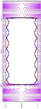
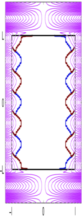
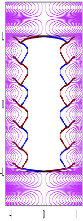
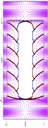
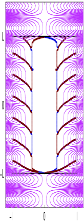
Figure 2: Running wave. Penetration of the magnetic field induced by an external current $\mathbf{J}_{e}=i_{e}(t)\sin\{k(y-vt)\}[\delta(x-a)-\delta(x+a)]\mathbf{e}_{z}$ into a cylindrical superconductor with the cross section $\Omega=\{-l\leq x\leq l,\ -L\leq y\leq L\}$. The wave amplitude $i_{e}$ grows linearly from zero at $t=0$ to its maximal value $i_{e0}$ at $t=t_{0}$ and then remains constant. The physical parameters: $l=1/k,\ L=10/k,\ a=1.1/k,\ t_{0}=4/kv,\ i_{e0}=J_{c}/k$. Shown for $t=[0.8,\ 1.6,\ 3.2,\ 5.6,\ 16.0]/kv$ are: the boundaries of plus- and minus critical current zones, the magnetic field lines, and the cylinder cross section. The parameters of numerical scheme: $50\times 500$ regular mesh of piecewise constant finite elements, time step $0.8/kv$.

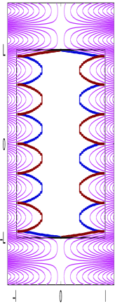
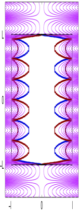
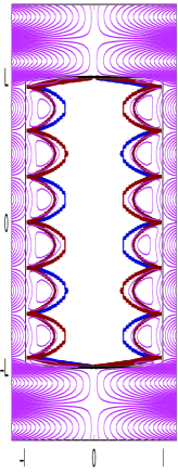
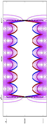
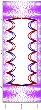
Figure 3: Standing wave. The external magnetic field is induced by the current $\mathbf{J}_{e}=i_{e}\sin(ky)\sin(2\pi ft)[\delta(x-a)-\delta(x+a)]\mathbf{e}_{z}$. Here $l=1/k,\ L=10/k,\ a=1.1/k,\ i_{e}=J_{c}/k$. Shown for $t=[0.24,\ 0.44,\ 0.56,\ 1.00,\ 1.12]/f$ are: the boundaries of plus- and minus critical current zones, the magnetic field lines, and the cylinder cross section. Regular finite element mesh $50\times 500$, time step $0.04/f$.

IV Asymptotic solution

Let an infinite slab $-l\leq x\leq l$ be placed into a magnetic field produced by the sheet current (10) or (11). We want to find the established periodic in time distribution of induced current density. It follows from (12) that the time-periodic part of current density we are interested in does not depend on the permanent part of external current. We set $I_{e}=0$ again just to simplify the consideration; this is not a limitation of the method employed.

It is not difficult to find a distribution of surface current density, $i_{s}(y,t)$, such that the current $i_{s}(y,t)[\delta(x+l)-\delta(x-l)]$ shields the superconductor from the external field. Clearly, complete shielding occurs if the magnetic vector potential of this current, $A_{s}$, compensates the external magnetic potential inside the superconductor,

$$A_{e}+A_{s}=0$$

for $-l<x<l$. Using expressions (14) and (15), we find that the shielding would be achieved if we set

$$i_{s}=-e^{-k(a-l)}i_{e}\sin\{k(y-vt)\},$$ (16)

$$i_{s}=-e^{-k(a-l)}i_{e}\sin(ky)\sin(2\pi ft)$$ (17)

for the running and standing waves, (10) and (11), respectively.

We now assume that the depth $\Delta$ to which fluctuations penetrate into the superconductor is much smaller than the fluctuation wavelength, $k\Delta\ll 1,$ interpret the shielding surface currents as the integrals of bulk current densities across a narrow penetration zone, and find the asymptotic distribution of bulk current density inside this zone analytically. First, let us note that for each $y$ the surface current $i_{s}(y,t)$ reaches its extremal values when the whole penetration zone (see Figs. 2 and 3) is occupied by the critical current density of the same sign. Therefore, the penetration depth can be calculated as $\Delta=\max(i_{s})/J_{c}$, which gives $\Delta=e^{-k(a-l)}i_{e}/J_{c}$ for the running wave and $\Delta(y)=e^{-k(a-l)}i_{e}|\sin(ky)|/J_{c}$ for the standing wave. We see that for both wave types the fluctuations may be regarded small if

$$\nu=k\Delta_{0}\ll 1,$$ (18)

where $\Delta_{0}=i_{e}e^{-k(a-l)}/J_{c}$.

If, at time $t$, the current $i_{s}(y,t)$ is neither maximal nor minimal, the penetration zone $-l\leq x\leq-l+\Delta$ (where $\Delta=\Delta_{0}$ for the running wave and $\Delta=\Delta_{0}|\sin(ky)|$ for the standing wave) contains regions of plus- and minus critical current densities. The near-surface region $-l<x<-l+\sigma(y,t)$ appears at the time when $\partial_{t}i_{s}(y,t)=0$ and, as it propagates inside, the current density there is $J_{c}\mbox{sign}\{\partial_{t}i_{s}(y,t)\}$. The rest of the penetration zone, $-l+\sigma(y,t)<x<-l+\Delta$, is occupied by the critical current density of the opposite sign. Comparing $i_{s}$ with the integral of current density across the penetration zone, we find the moving boundary $\sigma(y,t)$:

$$\sigma(y,t)=\frac{1}{2}\left(\Delta+\frac{i_{s}(y,t)}{J_{c}}\mbox{sign}\{\partial_{t}i_{s}(y,t)\}\right).$$ (19)

Near the slab surface $x=+l$ the current density distribution is antisymmetric.

Simple physical arguments were used above to obtain the asymptotic solutions for weak penetration: postulating the solution structure, we spread the shielding surface current into a bulk current in the near-surface zone. In a similar way, weak penetration of alternating uniform field into a perpendicular circular cylinder has been studied in [16, 17]. Although the chosen surface current would have shield the superconductor from the external magnetic field completely, spreading this current into the bulk makes shielding imperfect. As will be shown below, the remaining field is of the order $O(\nu)$. We will now extend our arguments and present the obtained asymptotic solutions as zero order terms of consistent asymptotic expansions.

IV-A Running wave

It is not difficult to see that the asymptotic distribution of current density inside the penetration zone $-l\leq x\leq-l+\Delta_{0}$, obtained for $\nu=k\Delta_{0}\ll 1$, can be presented as

$$J=-J_{c}S(k(y-vt)-\Psi_{0}(\varsigma/\Delta_{0})),\ \ \ \varsigma=x+l\in[0,\Delta_{0}],$$ (20)

where $S(z)=\mbox{sign}(\sin(z))$ is a $2\pi$-periodic step-function and $\Psi_{0}(u)=\arcsin(1-2u)$.

Let us now look for the current density

$$J=-J_{c}S(k(y-vt)-\Psi(\varsigma/\Delta)),\ \ \ \varsigma=x+l\in[0,\Delta]$$ (21)

where

$$\Delta=\Delta_{0}(1+r_{1}\nu+r_{2}\nu^{2}+...),$$ (22)

$$\Psi(u)=\Psi_{0}(u)+\nu\Psi_{1}(u)+\nu^{2}\Psi_{2}(u)+...$$ (23)

are such that the current (21), jointly with the opposite one near another superconductor surface, shield the external magnetic field.

We partly solve this problem in Appendix I by showing first that the vector potential produced by the zero-order approximation (20) to current density compensates the potential of external current inside the superconductor (but outside the penetration zone) up to the $O(\nu)$ terms; hence the external magnetic field inside the superconductor is shielded up to the same order in $\nu$. We find then the first order corrections, $r_{1}$ and $\Psi_{1}$, ensuring shielding of the magnetic field up to the second order, $O(\nu^{2})$.

It turns out (see Appendix I) that a nonsingular function $\Psi_{1}$ can be found only if $r_{1}=-\frac{1}{2}$, so the penetration depth becomes

$$\Delta=\Delta_{0}(1-\frac{1}{2}\nu+O(\nu^{2})).$$

It is further shown that the external magnetic field is shielded up to the second order in $\nu$ if

$$\Psi_{1}(\varsigma/\Delta)=\sum_{m=0}^{M}a_{m}U_{2m}(1-2\varsigma/\Delta),$$ (24)

where $U_{n}(\tau)=\sin((n+1)\arccos(\tau))/\sin(\arccos(\tau))$ are the Chebyshev polynomials of the second kind,

$$a_{m}=-\frac{1}{\pi}\left(\frac{1}{4(m+1)^{2}-1}+\frac{1}{4m^{2}-1}\right),$$ (25)

and $M$ satisfies the conditions

$$\nu\ln(M+1)\ll\pi$$

if $M>1$ (or $\nu\ll\pi$ if $M=0,1$) and

$$\frac{e^{-(2M+3)\nu}}{2M+1}\lesssim O(\nu).$$

The first of these conditions ensures that $|\nu\Psi_{1}|\ll 1$, the second provides for the $O(\nu^{2})$ shielding of magnetic field. The conditions are easy to satisfy and, usually, only a few terms of the series are needed. Thus, in the examples in Fig. 4, we used $M=1$ for $\nu=0.2$ and $M=0$ for $\nu=0.4$.

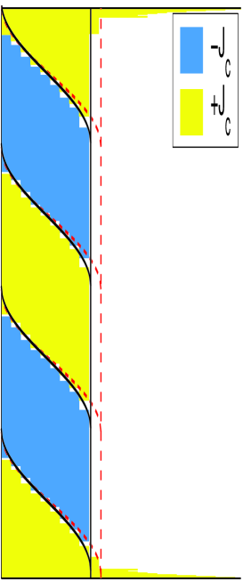
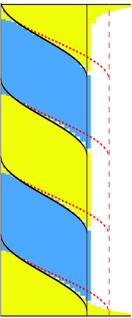
Figure 4: Penetration of the running wave fluctuations. Domains of plus- and minus critical current densities (numerical solution) and their asymptotic boundaries: ”- -” – zero order approximation, ”—” – first order approximation. Left: $i_{e}=0.25J_{c}/k$ and $\nu=0.2$; right: $i_{e}=0.5J_{c}/k$ and $\nu=0.4$. In both cases, $l=0.5/k,\ a=0.7/k,\ L=2\pi/k$. Different scales in x and y.

IV-B Standing wave

We find first a correction to the asymptotic penetration depth $\Delta(y)=\Delta_{0}|\sin(ky)|$. Let us choose a moment when the external field is the strongest, e.g., $t=T/4$, so that for each $y$ the induced current density is

$$J=-J_{c}S(ky),$$ (26)

in the whole penetration zone $0\leq\varsigma=x+l\leq\Delta(y)$ (and is opposite in the zone near another slab surface). We will now assume that

$$\Delta(y)=\Delta_{0}(|\sin(ky)|+\nu\Psi_{1}(ky)+\nu^{2}\Psi_{2}(ky)+...)$$ (27)

and find a correction $\Psi_{1}(s)$ that ensures better shielding of the external field for this moment of time.

It can be shown (see Appendix II) that the magnetic field is shielded up to the second order in $\nu$ if

$$\Psi_{1}(s)=-\frac{1}{\pi}\mbox{sign}(\sin(s))[2\sin(s)+\sin(2s)\ln(|\tan(s/2)|)].$$ (28)

Equations (26), (27), and (28) give the asymptotic distribution of current for $t=T/4$. It is now easy to obtain the solution for any time moment. Let, for example, $T/4<t<3T/4$. Then the closest to the surface $x=-l$ part of the penetration zone is occupied by the current density $+J_{c}S(ky)$. We can present this as a superposition of the current density $-J_{c}S(ky)$ in the whole penetration zone and the current $+2J_{c}S(ky)$ in the part of this zone near the surface. Up to the second order terms, the current $-J_{c}S(ky)$ shields the external current $i_{e}\sin(ky)[\delta(x+a)-\delta(x-a)]$, so the opposite current density $+2J_{c}S(ky)$ has to shield the external current $i_{e}(\sin(2\pi ft)-1)\sin(ky)[\delta(x+a)-\delta(x-a)]$. This means that the boundary between the two zones must be

$$\widetilde{\Delta}(y,t)=\frac{\Delta(y)}{2}(1-\sin(2\pi ft)).$$ (29)

In Fig. 5, we compare the numerical and asymptotic solutions for two values of parameter $\nu$. As in the running wave case, these solutions are close.

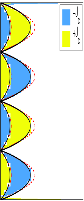
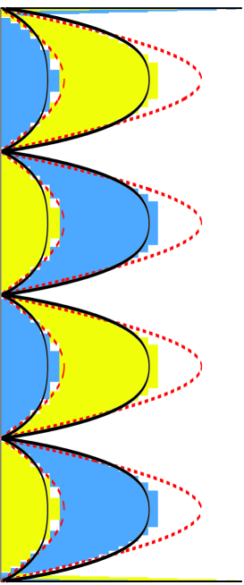
Figure 5: Penetration of the standing wave fluctuations. Notations and parameters as in the previous figure.

V AC losses

Let the external magnetic field be periodic in time, e.g., induced by a periodic current density $\mathbf{J}_{e}(r,t)$, and $T$ its period. Then there establishes a periodic induced current density in the superconductor, $\mathbf{J}(r,t)$. Suppose this latter function was found and it is needed to calculate the energy losses,

$$P=\frac{1}{T}\int_{0}^{T}\int_{\Omega}\mathbf{J}\cdot\mathbf{E}\,d\Omega dt=\frac{1}{T}\int_{0}^{T}\int_{\Omega}\rho\mathbf{J}^{2}\,d\Omega dt.$$

This would be an easy task for a usual conductor with the known resistivity. However, for type-II superconductors $\rho(r,t)$ is an effective resistivity caused by the movement of magnetic vortices and is not known a priory. Mathematically, in the Bean model, this is a dual variable excluded by transition to the variational formulation; accurate calculation of $\rho$ (or $\mathbf{E}$) in the general case is difficult. To avoid this complication, we employ a method based on the magnetic potential representation of electric field (6) and similar to those suggested in [17, 18] but applicable to nonuniform external fields.

Since $\mathbf{J}$ satisfies the zero divergence conditions (5), for any gauge holds

$$P=\frac{1}{T}\int_{0}^{T}\int_{\Omega}\mathbf{J}\cdot\mathbf{E}\,d\Omega dt=-\frac{1}{T}\int_{0}^{T}\int_{\Omega}\mathbf{J}\cdot\partial_{t}\mathbf{A}\,d\Omega dt=-\frac{\mu_{0}}{T}\int_{0}^{T}\int_{\Omega}\mathbf{J}\cdot G*\partial_{t}\mathbf{J}\,d\Omega dt-\frac{1}{T}\int_{0}^{T}\int_{\Omega}\mathbf{J}\cdot\partial_{t}\mathbf{A}_{e}\,d\Omega dt.$$

It is easy to see that

$$\int_{0}^{T}\int_{\Omega}\mathbf{J}\cdot G*\partial_{t}\mathbf{J}\,d\Omega dt=\int_{0}^{T}\frac{d}{dt}\left\{\frac{1}{2}\int_{\Omega}\mathbf{J}\cdot G*\mathbf{J}\,d\Omega\right\}dt=0$$

due to periodicity of $\mathbf{J}$. Hence we obtain

$$P=-\frac{1}{T}\int_{0}^{T}\int_{\Omega}\mathbf{J}\cdot\partial_{t}\mathbf{A}_{e}\,d\Omega dt$$

and, since the time period of the product $\mathbf{J}\cdot\partial_{t}\mathbf{A}_{e}$ is $T/2$, we can also write

$$P=-\frac{2}{T}\int_{t_{0}}^{t_{0}+T/2}\int_{\Omega}\mathbf{J}\cdot\partial_{t}\mathbf{A}_{e}\,d\Omega dt$$ (30)

for arbitrary time moment $t_{0}$.

V-A AC losses for running wave

Clearly, only half of the slab may be considered due to symmetry and we can now use (30) with $\Omega=(-l,0)$ and $T=2\pi/kv$ to find the asymptotic AC losses for small fluctuations. Obviously, the value of integral (30) must be the same for all $y$ and equal to the rate of AC losses per unit of slab surface. We neglect the second order terms in (22), (23) and assume

$$\Psi=\Psi_{0}+\nu\Psi_{1},\ \ \ \Delta=\Delta_{0}\left(1-\frac{\nu}{2}\right).$$ (31)

To simplify computations, let us take $y=0$, so that (21) gives

$$J|_{y=0}=J_{c}S(kvt+\Psi(\varsigma/\Delta)),\ \ \ \varsigma=x+l\in[0,\Delta],$$

and choose $t_{0}=-\Psi(0)/kv$. For small $\nu$ the function $\Psi(\varsigma/\Delta)$ is close to $\Psi_{0}(\varsigma/\Delta)$ and monotonically decreases for $\varsigma\in[0,\Delta]$. Therefore, $kvt_{0}+\Psi(\varsigma/\Delta)$ changes monotonically from zero at $\varsigma=0$ to $kvt_{0}+\Psi(1)=-\pi$ at $\varsigma=\Delta$. Indeed, since $\Psi_{1}(0)=\Psi_{1}(1)$, we have

$$\Psi(1)=\Psi_{0}(1)+\nu\Psi_{1}(1)=-\pi+\Psi_{0}(0)+\nu\Psi_{1}(0)=-\pi+\Psi(0).$$ (32)

Hence, for $y=0$ the whole penetration zone at $t=t_{0}$ is occupied by the current density $-J_{c}$. For $t_{0}<t<t_{0}+T/2$ there is a $+J_{c}$-current-density zone propagating inside and sweeping out the $-J_{c}$ zone at $t=t_{0}+T/2$. The moving boundary between the two zones is determined by the condition $kvt+\Psi(\varsigma/\Delta)=0$. Taking this into account we rewrite (30) as

$$P=-\frac{2J_{c}}{T}\int_{0}^{\Delta}\left.\left\{-\int_{-\Psi(0)/kv}^{-\Psi(\varsigma/\Delta)/kv}\partial_{t}A_{e}dt+\int_{-\Psi(\varsigma/\Delta)/kv}^{-\Psi(1)/kv}\partial_{t}A_{e}dt\right\}\right|_{\tiny\begin{array}[]{l}x=-l+\varsigma\\ y=0\end{array}}d\varsigma=$$

$$-\frac{2\mu_{0}i_{e}J_{c}\Delta}{kT}e^{-ka}\int_{0}^{1}[2\sin\Psi(u)-\sin\Psi(1)-\sin\Psi(0)]\sinh\left(-kl+\nu\frac{\Delta}{\Delta_{0}}u\right)du,$$

since $A_{e}(x,y,t)$ is given by (14). Note that $\sin\Psi(1)+\sin\Psi(0)=0$ because of (32); also $i_{e}e^{-ka}=J_{c}\Delta_{0}e^{-kl}$. Substituting $\Delta$ and $\Psi$ from (31) we obtain

$$P=\frac{4\mu_{0}J_{c}^{2}\Delta_{0}}{k^{2}T}P_{0},$$

where, up to the higher order terms,

$$\begin{split}P_{0}&=-\nu e^{-kl}\left(1-\frac{1}{2}\nu\right)\int_{0}^{1}\sin\{\arcsin(1-2u)+\nu\Psi_{1}(u)\}\sinh(-kl+\nu u)du\\ &=-\frac{\nu^{2}}{2}e^{-kl}\left[-\frac{1}{3}\cosh(-kl)+\sinh(-kl)\int_{-1}^{1}\Psi_{1}\left(\frac{1-\tau}{2}\right)\sqrt{1-\tau^{2}}d\tau\right]\end{split}$$ (33)

Here $\tau=1-2u$ and $\Psi_{1}$ is given by (24) as a finite series of the Chebyshev polynomials. We see that the leading AC loss term depends on the first order correction to solution (20). Since

$$\int_{-1}^{1}U_{2m}(\tau)\sqrt{1-\tau^{2}}d\tau=\left\{\begin{array}[]{ll}\frac{\pi}{2}&\ m=0,\\ 0&\ m>0\end{array}\right.$$

only the first term of the series (24) gives input into AC losses. We find

$$P_{0}=\frac{\nu^{2}}{2}e^{-kl}\left[\frac{1}{3}\cosh(-kl)-\frac{a_{0}\pi}{2}\sinh(-kl)\right]=\frac{\nu^{2}}{6}$$

and, finally, the asymptotic losses for weak penetration,

$$P=\frac{2\mu_{0}J_{c}^{2}\Delta_{0}}{3k^{2}T}\nu^{2}=\frac{2}{3}f\mu_{0}J_{c}^{2}\Delta_{0}^{3},$$ (34)

where $f=1/T$ is the frequency of fluctuations. Note that the expression obtained would coincide with the well known formula for hysteresis losses caused by fluctuations of spatially uniform external magnetic field (incomplete penetration), $P=\frac{2}{3}f\mu_{0}H_{0}^{3}/J_{c}$, if we rewrite this latter formula not for the fluctuation amplitude $H_{0}$ but using the penetration depth $\Delta_{0}$, equal to $H_{0}/J_{c}$ for the uniform field.

V-B AC losses for standing wave

To estimate the average asymptotic AC losses per unit of slab surface we modify slightly the formula (30) to calculate the density of these losses,

$$P(y)=-\frac{2}{T}\int_{T/4}^{3T/4}\int_{0}^{\Delta(y)}\partial_{t}A_{e}Jd\varsigma\,dt,$$

where $T=1/f$, then average over half the fluctuation wavelength,

$$\langle P\rangle=\frac{2}{\lambda}\int_{0}^{\lambda/2}P(y)dy,$$

where $\lambda=2\pi/k$. Assuming $T/4<t<3T/4$ and $0<y<\pi/k$ we get $J=+J_{c}$ for $0<\varsigma<\widetilde{\Delta}(y,t)$ and $J=-J_{c}$ for $\widetilde{\Delta}(y,t)<\varsigma<\Delta(y)$, where $\Delta(y)=\Delta_{0}(|\sin(ky)|+\nu\Psi_{1}(ky)+O(\nu^{2}))$ and $\widetilde{\Delta}(y,t)$ is given by (29). Substituting $I_{e}=0$, $x=-l+\varsigma$ into the vector potential (15) and integrating, we obtain

$$P(y)=-\frac{2J_{c}}{T}\int_{T/4}^{3T/4}\left\{\int_{0}^{\widetilde{\Delta}(y,t)}\partial_{t}A_{e}d\varsigma-\int_{\widetilde{\Delta}(y,t)}^{\Delta(y)}\partial_{t}A_{e}d\varsigma\right\}dt=\frac{4}{k^{2}}\mu_{0}fJ_{c}^{2}\Delta_{0}P_{0}(y),$$

where

$$P_{0}(y)=e^{-kl}\sin(ky)\left[\cosh(-kl)+\cosh\left(-kl+\nu\frac{\Delta(y)}{\Delta_{0}}\right)-\frac{\sinh\left(-kl+\nu\frac{\Delta(y)}{\Delta_{0}}\right)-\sinh(-kl)}{\frac{\nu\Delta(y)}{2\Delta_{0}}}\right].$$ (35)

For $0\leq y\leq\pi/k$ we have $\Delta(y)/\Delta_{0}=\sin(ky)+\nu\Psi_{1}(ky)+O(\nu^{2})$ and, up to the higher order terms,

$$P_{0}(y)=e^{-kl}\left[\frac{\nu^{2}}{6}\sin^{3}(ky)\cosh(kl)+\nu^{3}\left(\frac{1}{3}\Psi_{1}(ky)\sin^{2}(ky)\cosh(kl)-\frac{1}{12}\sin^{4}(ky)\sinh(kl)\right)\right].$$

Except for the points very close to $y=0$ or $\pi/k$, where the term containing $\Psi_{1}(ky)$ dominates but the losses are negligible,

$$P(y)\approx\frac{2}{3k^{2}}\mu_{0}fJ_{c}^{2}\Delta_{0}\nu^{2}\sin^{3}(ky)e^{-kl}\cosh(kl)=\frac{2}{3}\mu_{0}fJ_{c}^{2}\Delta_{0}^{3}(y)\sin^{3}(ky)\frac{1+e^{-2kl}}{2}.$$ (36)

This is close to the density of losses in an alternating uniform field if $kl\ll 1$ and is twice smaller if $kl\gg 1$, provided the penetration depth is the same. Finally, we find the asymptotic average AC losses per unit of slab surface for the standing wave fluctuations:

$$\langle P\rangle=\frac{4(1+e^{-2kl})}{9\pi}\mu_{0}f\Delta_{0}^{3}J_{c}^{2}.$$ (37)

We see that in this case the leading asymptotic AC loss term is determined by the zero order approximation to current density distribution and does not depend on the first order correction as in the running wave case.

VI Discussion

Magnetic field fluctuations are inevitable in most practical applications of superconductors. In this work we used the Bean critical state model to study the effect of spatially nonuniform fluctuations of the external magnetic field. Although solutions have been obtained only for two model situations, they help to understand qualitatively the effect of nonuniform fluctuations in general. The asymptotic estimates, derived for small spatially nonuniform fluctuations using a general gauge-invariant formula for AC losses, are the main result of our work.

For an alternating uniform magnetic field the AC losses in a superconductor are usually expressed via the amplitude of field variations. This is inconvenient if the external field is nonuniform. Typically, as for the configurations considered in our work, both the magnitude and direction of the external field depend on position, time, problem geometry, and the fluctuation wavelength. It seems difficult to relate the losses to any specific characteristic of this field. The lack of a universal direct relation between the external field at the surface of a superconductor and AC losses becomes even more apparent if we consider, for example, a hollow superconductive cylinder with a long coil placed into its hole [19]. An alternating coil current induces the shielding current in the superconductor because the magnetic flux changes. Nevertheless, had the superconductor been removed, the same coil current would produce no magnetic field outside the coil at all.

Because of this reason the formulas for AC losses in this work are presented in terms of the depth to which fluctuations penetrate into the superconductor. To determine this depth and the induced current density asymptotically for small fluctuations, we found first the shielding surface current. Spreading this current into the bulk and taking into account the current density constraint, we were able to obtain the zero order approximation to current density which was then further improved.

Such an approach is not limited to slab configuration and the two types of fluctuations considered above. Thus, using the method derived recently by Bhagwat and Karmakar [20], one can find the surface current shielding a cylinder of an arbitrary given cross section placed into a uniform external magnetic field. This makes possible to extend, following the scheme used in our work, the asymptotic solution for cylinders in alternating uniform transverse field [16, 17] to cylinders with non-circular cross sections (in this case the penetration is weak if its depth is much smaller than the characteristic cross section size).

The results obtained enable one to estimate AC losses in superconductors of magnetic bearings and levitation systems, where the typical configuration is similar to that of a running wave fluctuations of external field near the surface of a thick slab ($kl\gg 1$, one-sided action of a nonuniform external field). Suppose we can remove the superconductor and measure the tangential component of field fluctuations at the position of slab surface. Let us approximate this component by a running wave with an amplitude $H_{t}$. By the method of images, surface current shielding these fluctuations has the amplitude $2H_{t}$. This can be used to estimate the penetration depth, $\Delta_{0}\approx 2H_{t}/J_{c}$. The losses can now be approximated using the formula (34) derived for the running wave fluctuations.

Numerical simulations based on a variational reformulation of the critical-state model helped us to envision solution structures and to control accuracy of asymptotic solutions. The asymptotic solutions, obtained at first by means of simple physical arguments, were presented as zero-order terms of a consistent asymptotic expansion. Finding the first order correction allowed us to improve these solutions. It has been shown that the correction ensures shielding of external magnetic field up to the second order, $H/H_{e}\sim O(\nu^{2})$, and (see Figs. 4, 5) provides for a satisfactory approximation for small parameter values up to $\nu\sim 0.4$. For both the running and standing wave fluctuations, the maximal penetration depth $\Delta_{max}$ is smaller than the value $\Delta_{0}$ given by zero order approximation: we found $\Delta_{max}\approx\Delta_{0}(1-\frac{\nu}{2})$ in the first case, $\Delta_{max}\approx\Delta_{0}(1-\frac{2\nu}{\pi})$ in the second one.

Expressed via the penetration depth, AC losses for running wave fluctuations (34) are given by exactly the same formula as AC losses for uniform field fluctuations. We cannot expect such a coincidence also for standing wave fluctuations, since the penetration zone depth is not constant in that case. However, the local losses (36) are close if $kl\ll 1$, which simply means that, locally, the long-wave limit is similar to the uniform fluctuations case. If the wavelength is shorter, the losses can be at most twice smaller than in the uniform case for the same local penetration depth. Using the average penetration depth, $\langle\Delta\rangle=2\Delta_{0}/\pi$, we can present the average losses (37) as $\langle P\rangle=\frac{2}{3}C\mu_{0}fJ_{c}^{2}\langle\Delta\rangle^{3},$ where $C=\pi^{2}(1+e^{-2kl})/12$. Since $0.82\leq C\leq 1.64$, the average losses are also close to AC losses in the uniform field case.

For standing wave fluctuations, the leading AC loss term is determined by zero order approximation to current density distribution, i.e., an approximation that is comparatively easy to find. This is similar to the case of uniform field fluctuations considered earlier in [17]. It is, therefore, surprising that the situation is different for the running-wave type of fluctuations: here knowledge of the first order correction to such a solution is necessary. Neglecting this correction would cause an error of the same order as the AC loss value itself.

To explain this discrepancy, let us note that the expressions (33) and (35) for AC losses for running and standing waves, respectively, have different structures. In (35), the small parameter appears only in a combination $\nu\Delta(y)/\Delta_{0}=\nu\Psi(y)$, where $\Psi=\Psi_{0}+\nu\Psi_{1}+...$ We can write $P_{0}(y)={\cal F}(y,\nu\Psi(y))$ and check that the function ${\cal F}(y,u)$ satisfies ${\cal F}(y,0)={\cal F}_{u}(y,0)=0$. Hence $P_{0}(y)=\frac{\nu^{2}}{2}{\cal F}_{uu}(y,0)\Psi_{0}^{2}(y)+O(\nu^{3})$; the main term does not depend on $\Psi_{1}$.

In the running wave case, the dependance on small parameter is different because the penetration depth and the shape of the free boundary are separated. The equation (33) can be written as $P_{0}=\nu{\cal F}(\nu,\Psi),$ where ${\cal F}$ is a functional and $\Psi=\Psi_{0}+\nu\Psi_{1}+...$ as in the previous case. Expanding we get $P_{0}=\nu{\cal F}(0,\Psi_{0})+\nu^{2}[{\cal F}_{\nu}(0,\Psi_{0})+({\cal F}_{\Psi}(0,\Psi_{0}),\Psi_{1})]+O(\nu^{3}).$ Here ${\cal F}_{\Psi}$ is the Frèchet derivative, the first term turns out to be zero, and so the leading term depends on $\Psi_{1}$.

In both cases, however, the leading term of AC losses is proportional to $\Delta_{0}^{3}$, which corresponds to $P\sim H^{3}$ dependance known for the uniform field fluctuations. The next approximation would lead to a deviation from cubic law. In the frame of the Bean model, such deviation can be due to the shape of a superconductor being different from that of a slab [6, 19], heating caused by AC losses [6], or, as in the present case, because of spatial non-uniformity of the external field.

Appendix A

The vector potential of the current (21) and the opposite one near $x=+l$ can be written as

$$A_{i}=\mu_{0}G*J=\frac{\mu_{0}J_{c}}{4\pi}\int_{-\infty}^{\infty}\int_{0}^{\Delta}S(k(y^{\prime}-vt)-\Psi(\varsigma/\Delta))\ln\left(\frac{(x+l-\varsigma)^{2}+(y-y^{\prime})^{2}}{(x-l+\varsigma)^{2}+(y-y^{\prime})^{2}}\right)d\varsigma\,dy^{\prime}.$$

Changing the variables, $u=\varsigma/\Delta$, $s=k(y^{\prime}-vt)-\Psi(u)$, and using the Taylor expansion we obtain:

$$A_{i}=\frac{\mu_{0}J_{c}}{4k\pi}\Delta_{0}(1+r_{1}\nu+...)\int_{-\infty}^{\infty}S(s)\int_{0}^{1}\ln\left(\frac{[k(x+l)-\nu\frac{\Delta}{\Delta_{0}}u]^{2}+[k(y-vt)-s-\Psi(u)]^{2}}{[k(x-l)+\nu\frac{\Delta}{\Delta_{0}}u]^{2}+[k(y-vt)-s-\Psi(u)]^{2}}\right)du\,ds=$$

$$=\frac{\mu_{0}h_{0}}{2k\pi}\left[A_{0}+A_{1}\nu+O(\nu^{2})\right].$$ (38)

Here

$$h_{0}=\frac{i_{e}}{2}e^{-k(a-l)}$$ (39)

is introduced as a characteristic magnitude of external field fluctuations at the surface of the superconductor and

$$A_{0}=\int_{0}^{1}D(x,y,t,u)du,\ \ \ \ A_{1}=\int_{0}^{1}uF_{1}(x,y,t,u)du+\int_{0}^{1}\Psi_{1}(u)F_{2}(x,y,t,u)du+r_{1}A_{0},$$

where

$$D=\int_{-\infty}^{\infty}S(s)\ln\left(\frac{[k(x+l)]^{2}+(\Gamma-s)^{2}}{[k(x-l)]^{2}+(\Gamma-s)^{2}}\right)ds,$$

$$F_{1}=-2\int_{-\infty}^{\infty}S(s)\left(\frac{k(x+l)}{(\Gamma-s)^{2}+[k(x+l)]^{2}}+\frac{k(x-l)}{(\Gamma-s)^{2}+[k(x-l)]^{2}}\right)ds,$$

$$F_{2}=2\int_{-\infty}^{\infty}S(s)(\Gamma-s)\left(-\frac{1}{(\Gamma-s)^{2}+[k(x+l)]^{2}}+\frac{1}{(\Gamma-s)^{2}+[k(x-l)]^{2}}\right)ds,$$

$$\Gamma=k(y-vt)-\Psi_{0}(u).$$

To calculate the integrals we present the periodic function $S$ as the Fourier series,

$$S(s)=\sum_{n=1}^{\infty}b_{n}\sin(ns),\ \ \ \ b_{n}=\left\{\begin{array}[]{ll}\frac{4}{\pi n}&\ n=2m+1,\\ 0&\ n=2m\end{array}\right.$$

and obtain

$$D=4\pi\sum_{n=1}^{\infty}\frac{b_{n}}{n}e^{-nkl}\sinh(nkx)\sin(n\Gamma),$$

$$F_{1}=4\pi\sum_{n=1}^{\infty}b_{n}e^{-nkl}\sinh(nkx)\sin(n\Gamma),\ \ F_{2}=-4\pi\sum_{n=1}^{\infty}b_{n}e^{-nkl}\sinh(nkx)\cos(n\Gamma).$$

We further obtain

$$A_{0}=4\pi\sum_{n=1}^{\infty}\frac{b_{n}}{n}e^{-nkl}\sinh(nkx)[\alpha_{n}\sin(nk(y-vt))-\beta_{n}\cos(nk(y-vt))],$$

where $b_{n}=0$ for all even $n$ and, for odd $n$,

$$\alpha_{n}=\int_{0}^{1}\cos(n\Psi_{0}(u))du=\left\{\begin{array}[]{ll}\pi/4,&n=1,\\ 0&n>1\end{array}\right.\ \ \ \ \ \ \beta_{n}=\int_{0}^{1}\sin(n\Psi_{0}(u))du=0.$$

Hence,

$$A_{0}=4\pi e^{-kl}\sinh(kx)\sin(k(y-vt)).$$ (40)

Similarly,

$$\begin{split}A_{1}=&4\pi\sum_{n=1}^{\infty}b_{n}e^{-nkl}\sinh(nkx)[\gamma_{n}\sin(nk(y-vt))-\delta_{n}\cos(nk(y-vt))]\\ &+r_{1}4\pi e^{-kl}\sinh(kx)\sin(k(y-vt)),\end{split}$$ (41)

where all even series terms are zero and, for n odd,

$$\gamma_{n}=\int_{0}^{1}u\cos(n\Psi_{0}(u))du-\int_{0}^{1}\Psi_{1}(u)\sin(n\Psi_{0}(u))du,$$ (42)

$$\delta_{n}=\int_{0}^{1}u\sin(n\Psi_{0}(u))du+\int_{0}^{1}\Psi_{1}(u)\cos(n\Psi_{0}(u))du.$$ (43)

We can now substitute the expressions (40) and (41) into (38), use (14) with $I_{e}=0$, and calculate the total magnetic field inside the superconductor but outside the penetration zone. We see that $A=A_{e}+A_{i}=\frac{\mu_{0}h_{0}}{2k\pi}(\nu A_{1}+O(\nu^{2}))$. Therefore, up to the second order terms,

$$\begin{split}H_{x}=&2\nu h_{0}\{r_{1}e^{-kl}\sinh(kx)\cos(k(y-vt))+\\ \ &\sum_{n=1}^{\infty}nb_{n}e^{-nkl}\sinh(nkx)[\gamma_{n}\cos(nk(y-vt))+\delta_{n}\sin(nk(y-vt))]\},\end{split}$$

$$\begin{split}H_{y}=&-2\nu h_{0}\{r_{1}e^{-kl}\cosh(kx)\sin(k(y-vt))+\\ \ &\sum_{n=1}^{\infty}nb_{n}e^{-nkl}\cosh(nkx)[\gamma_{n}\sin(nk(y-vt))-\delta_{n}\cos(nk(y-vt))]\}.\end{split}$$

This proves that the current density (20) shields the external field up to the first order in $\nu$ and is a zero order approximation. To nullify the first order terms of magnetic field we will now try to satisfy the conditions

$$\gamma_{n}=\left\{\begin{array}[]{ll}-r_{1}/b_{1}&\ n=1,\\ 0&\ n>1,\end{array}\right.\ \ \ \mbox{and}\ \ \ \delta_{n}=0,$$ (44)

for odd values of $n$. Since $\Psi_{0}(u)=\arcsin(1-2u)$, we denote $\tau=1-2u$ and express $\sin(n\Psi_{0}(u))$ and $\cos(n\Psi_{0}(u))$ in (42), (43) via the Chebyshev polynomials of the first and second kind,

$$T_{n}(\tau)=\cos(n\arccos\tau),\ \ \ U_{n}(\tau)=\sin((n+1)\arccos\tau)/\sin(\arccos\tau),$$

correspondingly,  for $\tau\in[-1,1]$. It can be shown that, for n odd,

$$\sin(n\arcsin\tau)=(-1)^{\frac{n-1}{2}}T_{n}(\tau),\ \ \ \cos(n\arcsin\tau)=(-1)^{\frac{n-1}{2}}U_{n-1}(\tau)\sqrt{1-\tau^{2}}.$$

Defining $\psi_{1}(\tau)$ as $\Psi_{1}(\frac{1-\tau}{2})=\Psi_{1}(u)$ and calculating the integrals of known functions, we obtain

$$\begin{array}[]{c}\gamma_{n}=\frac{1}{2}(-1)^{\frac{n-1}{2}}\left(\int_{-1}^{1}\frac{1-\tau}{2}U_{n-1}(\tau)\sqrt{1-\tau^{2}}d\tau-\int_{-1}^{1}\psi_{1}(\tau)T_{n}(\tau)d\tau\right)=\\ \frac{1}{2}(-1)^{\frac{n-1}{2}}\left(\left\{\begin{array}[]{ll}\pi/4&\ n=1,\\ 0&\ n>1\end{array}\right\}-\int_{-1}^{1}\psi_{1}(\tau)T_{n}(\tau)d\tau\right)\end{array}$$

$$\begin{array}[]{c}\delta_{n}=\frac{1}{2}(-1)^{\frac{n-1}{2}}\left(\int_{-1}^{1}\frac{1-\tau}{2}T_{n}(\tau)d\tau+\int_{-1}^{1}\psi_{1}(\tau)U_{n-1}(\tau)\sqrt{1-\tau^{2}}d\tau\right)=\\ \frac{1}{2}(-1)^{\frac{n-1}{2}}\left(d_{n}+\int_{-1}^{1}\psi_{1}(\tau)U_{n-1}(\tau)\sqrt{1-\tau^{2}}d\tau\right),\end{array}$$

where $n$ is odd and

$$d_{n}=\frac{1}{2}\left[\frac{1}{(n+1)^{2}-1}+\frac{1}{(n-1)^{2}-1}\right].$$

We can now rewrite the conditions (44) as

$$\int_{-1}^{1}\psi_{1}(\tau)T_{n}(\tau)d\tau=\left\{\begin{array}[]{ll}\frac{\pi}{4}\left(\frac{1}{2}+r_{1}\right)&n=1,\\ 0&n>1\end{array}\right.$$ (45)

$$\int_{-1}^{1}\psi_{1}(\tau)U_{n-1}(\tau)\sqrt{1-\tau^{2}}d\tau=-d_{n}$$ (46)

and use them to determine $\psi_{1}(\tau)$ and $r_{1}$. Let us present $\psi_{1}$ as the sum of its even and odd parts, $\psi_{1}^{e}$ and $\psi_{1}^{o}$. Since functions $T_{n}$ are odd for odd n, even for even n, and orthogonal on $[-1,1]$ with the weight $1/\sqrt{1-\tau^{2}}$, condition (45) means that $\psi_{1}^{o}(\tau)\sqrt{1-\tau^{2}}=cT_{1}(\tau)$ where $T_{1}(\tau)=\tau$ and

$$c={\frac{\pi}{4}\left(\frac{1}{2}+r_{1}\right)}\left/\int_{-1}^{1}\frac{T_{1}^{2}(\tau)d\tau}{\sqrt{1-\tau^{2}}}\right.=\frac{1}{2}\left(\frac{1}{2}+r_{1}\right).$$

Thus $\psi_{1}^{o}=c\tau/\sqrt{1-\tau^{2}}$ and is singular at $\tau=\pm 1$ if $c\neq 0$. Since the expansion (38) is valid only for $|\nu\Psi_{1}(u)|\ll 1$, we need a nonsingular function and must set

$$r_{1}=-\frac{1}{2}$$

to make $c=0$. This determines the first order correction to the penetration depth:

$$\Delta=\Delta_{0}(1-\frac{1}{2}\nu+O(\nu^{2})).$$

The function $\psi_{1}$ becomes even and we can expand it into a series of the Chebyshev polynomials of the second kind containing only the polynomials of even orders:

$$\psi_{1}(\tau)=\sum_{m=0}^{\infty}a_{m}U_{2m}(\tau).$$ (47)

The polynomials $U_{n}$ are orthogonal on $[-1,1]$ with the weight $\sqrt{1-\tau^{2}}$, so the coefficients of this series are easily found from the condition (46):

$$a_{m}=-d_{2m+1}\left/\int_{-1}^{1}U_{2m}^{2}(\tau)\sqrt{1-\tau^{2}}d\tau\right.=-\frac{1}{\pi}\left(\frac{1}{4(m+1)^{2}-1}+\frac{1}{4m^{2}-1}\right).$$

We have now satisfied the conditions (44) but there appears a contradiction: although the series (47) converges for $\tau\in(-1,1)$, $\psi_{1}$ becomes infinite at $\tau=\pm 1$. Indeed, at these points $U_{2m}=2m+1$ and $a_{m}\approx-1/2\pi m^{2}$ for big $m$. Since the conditions (44) were derived under assumption $|\nu\Psi_{1}(u)|\ll 1$, the function determined by this series cannot be accepted as the first order correction to $\Psi_{0}$.

The computations, however, were not in vain and this singularity can be eliminated, if we take only a finite number of terms and define

$$\psi_{1}(\tau)=\sum_{m=0}^{M}a_{m}U_{2m}(\tau).$$ (48)

It can be shown that in this case $|\psi_{1}(\tau)|<\ln(M+1)/\pi$ for all $M>1$ and $|\psi_{1}(\tau)|<16/15\pi$ for $M=0$ or $1$. Thus, the assumption remains valid provided that

$$\left\{\begin{array}[]{ll}\nu\ln(M+1)\ll\pi&\ \mbox{if}\ M>1,\\ \nu\ll\pi&\ \mbox{if}\ M=0,1.\end{array}\right.$$ (49)

It is easy to see that conditions (44) for $\gamma_{n}$ are still satisfied for all $n$, whereas the conditions for $\delta_{n}$ hold only for $n\leq 2M+1$. For $n>2M+1$ we have

$$\delta_{n}=\frac{1}{2}(-1)^{\frac{n-1}{2}}d_{n}\approx\frac{1}{2n^{2}}(-1)^{\frac{n-1}{2}}.$$

The non-compensated magnetic field inside the superconductor has, up to the second order in $\nu$, the components

$$\begin{split}H_{x}&=2\nu h_{0}\sum_{n=2M+3}^{\infty}nb_{n}\delta_{n}e^{-nkl}\sinh(nkx)\sin(nk(y-vt)),\\ H_{y}&=2\nu h_{0}\sum_{n=2M+3}^{\infty}nb_{n}\delta_{n}e^{-nkl}\cosh(nkx)\cos(nk(y-vt)).\end{split}$$

For $|x|<l-\Delta_{0}$ we have $e^{-nkl}\cosh(nkx)<e^{-n\nu}$, $e^{-nkl}|\sinh(nkx)|<e^{-n\nu}$; also $nb_{n}=4/\pi$ for odd $n$. Hence,

$$|H_{x}|,|H_{y}|\lesssim\nu h_{0}\frac{4}{\pi}\sum_{m=M+1}^{\infty}\frac{e^{-(2m+1)\nu}}{(2m+1)^{2}}<\nu h_{0}\frac{4}{\pi}e^{-(2m+3)\nu}\int_{M}^{\infty}\frac{dm}{(2m+1)^{2}}<\nu h_{0}\frac{2e^{-(2M+3)\nu}}{\pi(2M+1)}$$

which proves that the field can be made $O(\nu^{2})$ if

$$\frac{e^{-(2M+3)\nu}}{2M+1}\lesssim O(\nu).$$ (50)

This means that the first order correction to $\Psi_{0}(u)$ may be chosen as $\Psi_{1}(u)=\psi_{1}(1-2u)$, where $\psi_{1}(\tau)$ is given by (48) and $M$ satisfies the conditions (49) and (50).

Appendix B

The vector potential of the current (26) can be written as

$$A_{i}=\frac{\mu_{0}J_{c}}{4\pi}\int_{-\infty}^{\infty}\int_{0}^{\Delta(y^{\prime})}S(ky^{\prime})\ln\left(\frac{(x+l-\varsigma)^{2}+(y-y^{\prime})^{2}}{(x-l+\varsigma)^{2}+(y-y^{\prime})^{2}}\right)d\varsigma\,dy^{\prime}.$$

Changing the variables, $u=\varsigma/\Delta(y^{\prime})$ and $s=ky^{\prime}$, we obtain

$$A_{i}=\frac{\mu_{0}J_{c}}{4k\pi}\int_{-\infty}^{\infty}S(s)\Delta(s/k)\left\{\int_{0}^{1}\ln\left(\frac{[k(x+l)-\nu\frac{\Delta(s/k)}{\Delta_{0}}u]^{2}+(s-ky)^{2}}{[k(x-l)+\nu\frac{\Delta(s/k)}{\Delta_{0}}u]^{2}+(s-ky)^{2}}\right)du\right\}ds$$

with $S(s)\Delta(s/k)=\Delta_{0}(\sin(s)+\nu\Psi_{1}(s)S(s)+...)$. Integrating in $u$ and expanding we get

$$A_{i}=\frac{\mu_{0}h_{0}}{2k\pi}[A_{0}+A_{1}\nu+O(\nu^{2})],$$

where the characteristic amplitude of fluctuations $h_{0}$ is defined by (39),

$$A_{0}=\int_{-\infty}^{\infty}\ln\left(\frac{[k(x+l)]^{2}+(s-ky)^{2}}{[k(x-l)]^{2}+(s-ky)^{2}}\right)\sin(s)\,ds=4\pi e^{-kl}\sin(ky)\sinh(kx),$$

$$\begin{split}A_{1}=&\int_{-\infty}^{\infty}\Psi_{1}(s)S(s)\ln\left(\frac{[k(x+l)]^{2}+(s-ky)^{2}}{[k(x-l)]^{2}+(s-ky)^{2}}\right)\,ds-\\ &\int_{-\infty}^{\infty}\left\{\frac{k(x+l)}{[k(x+l)]^{2}+(s-ky)^{2}}+\frac{k(x-l)}{[k(x-l)]^{2}+(s-ky)^{2}}\right\}\sin(s)|\sin(s)|\,ds.\end{split}$$ (51)

Obviously, $\Psi_{1}$ should be a $\pi$-periodic and even (because of symmetry) function. To calculate the integrals in (51) we present $\Psi_{1}(s)S(s)$ and $|\sin(s)|\sin(s)$ as the Fourier series,

$$\Psi_{1}(s)S(s)=\sum_{n=1}^{\infty}a_{n}\sin(ns),\ \ \ \ \ |\sin(s)|\sin(s)=\sum_{n=1}^{\infty}b_{n}\sin(ns),$$

where $b_{n}=-\frac{8}{\pi n(n^{2}-4)}$ for odd $n$, $b_{n}=0$ for even $n$, and the coefficients $a_{n}$ are unknown. Integrating, we find

$$A_{1}=2\pi\sum_{n=1}^{\infty}\left(\frac{2}{n}a_{n}+b_{n}\right)e^{-knl}\sin(nky)\sinh(nkx).$$

Up to $O(\nu^{2})$, the total magnetic potential can be written as

$$A=A_{e}+A_{i}=\nu\frac{\mu_{0}h_{0}}{2k\pi}A_{1}=\nu\frac{\mu_{0}h_{0}}{k}\sum_{n=1}^{\infty}\left(\frac{2}{n}a_{n}+b_{n}\right)e^{-knl}\sin(nky)\sinh(nkx).$$

To make zero the $O(\nu)$ terms of magnetic field inside the superconductor, it is sufficient to satisfy the conditions

$$a_{n}=-n\frac{b_{n}}{2}=\left\{\begin{array}[]{lc}\frac{4}{\pi(n^{2}-4)}&\ n=2m+1,\\ 0&n=2m.\end{array}\right.$$

This gives

$$\Psi_{1}(s)S(s)=\sum_{m=0}^{\infty}a_{2m+1}\sin(\{2m+1\}s)$$

and so, up to the second order terms, the penetration depth can be presented as

$$\Delta(y)=\Delta_{0}\{|\sin(ky)|+\nu V(ky)\mbox{sign}[\sin(ky)]\},$$

where the series

$$V(s)=\frac{4}{\pi}\sum_{m=0}^{\infty}\frac{\sin(\{2m+1\}s)}{(2m+1)^{2}-4}$$

can be summed up analytically. Let us denote $z=e^{is}$,

$$U(s)=\frac{4}{\pi}\sum_{m=0}^{\infty}\frac{\cos(\{2m+1\}s)}{(2m+1)^{2}-4},$$

and consider the complex function

$$\begin{split}{\cal W}=&U(s)+iV(s)=\frac{4}{\pi}\sum_{m=0}^{\infty}\frac{z^{2m+1}}{(2m+1)^{2}-4}=\frac{1}{\pi}\sum_{m=0}^{\infty}z^{2m+1}\left[\frac{1}{2m-1}-\frac{1}{2m+3}\right]=\\ \ &\frac{1}{\pi}\left[\frac{1}{z}-z+\left(z^{2}-\frac{1}{z^{2}}\right)\sum_{m=1}^{\infty}\frac{z^{2m-1}}{2m-1}\right]=\frac{1}{\pi}\left[\frac{1}{z}-z+\left(z^{2}-\frac{1}{z^{2}}\right)\sum_{m=1}^{\infty}\int_{0}^{z}z^{2m-2}dz\right]=\\ \ &\frac{1}{\pi}\left[\frac{1}{z}-z+\left(z^{2}-\frac{1}{z^{2}}\right)\int_{0}^{z}\frac{dz}{1-z^{2}}\right]=\frac{1}{\pi}\left[\frac{1}{z}-z+\left(z^{2}-\frac{1}{z^{2}}\right)\frac{1}{2}\ln\left(\frac{1+z}{1-z}\right)\right].\end{split}$$

Since $z-1/z=2i\sin(s),\ z^{2}-1/z^{2}=2i\sin(2s)$, and $Re\left[\ln\left(\frac{1+z}{1-z}\right)\right]=-\ln(|\tan(s/2)|)$, the imaginary part of ${\cal W}$ is

$$V(s)=-\frac{2}{\pi}\sin(s)-\frac{1}{\pi}\sin(2s)\ln(|\tan(s/2)|).$$

References

• [1] K. Takase, S. Shindo, K. Demachi, and K. Miya, “A study on the relaxation of levitation property in an HTSC magnetic bearing,” in Proceedings of the 1 Japanese-Greek Joint Workshop on Superconductivity and Magnetic Materials, A. G. Mamalis, K. Miya, M. Enokizono, and A. Kladas, Eds., Athens, Greece, 1999.
• [2] E. H. Brandt, “Superconductors of finite thickness in a perpendicular magnetic field: Strips and slabs,” Phys. Rev. B, vol. 54, no. 6, pp. 4246–4264, 1996.
• [3] ——, “Superconductor disks and cylinders in an axial magnetic field. I. Flux penetration and magnetization curves,” Phys. Rev. B, vol. 58, no. 10, pp. 6506–6522, 1998.
• [4] L. Prigozhin, “Analysis of critical-state problems in type-II superconductivity,” IEEE Trans. Appl. Superconduct., vol. 7, no. 4, pp. 3866–3873, 1997.
• [5] M. Maslouh, F. Bouillault, A. Bossavit, and J.-C. Vérité, “From Bean’s model to the h-m characteristic of a superconductor: Some numerical experiments,” IEEE Trans. Appl. Supercond., vol. 7, no. 3, pp. 3797–3801, 1997.
• [6] V. Sokolovsky and V. Meerovich, AC Losses in Bulk High Temperature Superconductors, ser. Studies of High Temperature Superconductors.   New York: Nova Science, 1998, vol. 32, pp. 79–132.
• [7] C. Bean, “Magnetization of high-field superconductors,” Rev. Mod. Phys., vol. 36, no. 1, pp. 31–39, 1964.
• [8] L. Prigozhin, “On the Bean critical-state model in superconductivity,” European J. Appl. Math., vol. 7, no. 3, pp. 237–248, 1996.
• [9] G. Duvaut and J.-L. Lions, Les Inéquations en Mécanique et Physique.   Paris: Dunod, 1972.
• [10] R. Glowinsky, J.-L. Lions, and R. Trémolièr, Numerical Analysis of Variational Inequalities.   Amsterdam: North-Holland, 1981.
• [11] R. Albanese and G. Ribonacci, Finite element methods for the solution of 3D eddy current problems, ser. Advances in Imaging and Electron Physics.   Academic Press, 1998, vol. 102, pp. 1–86.
• [12] A. Bossavit, Computational Electromagnetism.   San Diego: Academic Press, 1998.
• [13] ——, “Numerical modelling of superconductors in three dimensions: A model and a finite element method,” IEEE Trans. Magn., vol. 30, no. 5, pp. 3363–3366, 1994.
• [14] L. Prigozhin, “The Bean model in superconductivity: Variational formulation and numerical solution,” J. Comput. Phys., vol. 129, no. 1, pp. 190–200, 1996.
• [15] Y. B. Kim, C. F. Hempstead, and A. R. Strnad, “Critical persistent currents in hard superconductors,” Phys. Rev. Lett., vol. 9, no. 7, pp. 306–309, 1962.
• [16] W. J. Carr, Jr., M. S. Walker, and J. H. Murphy, “Alternating field loss in a multifilament superconducting wire for weak AC fields superposed on a constant bias,” J. Appl. Phys., vol. 46, no. 9, pp. 4048–4052, 1975.
• [17] M. Ashkin, “Flux distribution and hysteresis loss in a round superconducting wire for the complete range of flux-penetration,” J. Appl. Phys., vol. 50, no. 11, pp. 7060–7066, 1979.
• [18] A. Bossavit, “Remarks about hysteresis in superconductivity modelling,” Physica B, vol. 142, no. 1-3, pp. 142–149, 2000.
• [19] V. Meerovich, V. Sokolovsky, S. Goren, and G. Jung, “AC losses in high-temperature superconductor BSCCO hollow cylinders with induced current,” Physica C, vol. 319, no. 3-4, pp. 238–248, 1999.
• [20] K. V. Bhagwat and D. Karmakar, “Current density on an arbitrary cylindrical surface producing transverse uniform interior field,” Europhys. Lett., vol. 49, no. 6, pp. 715–721, 2000.