On the crescentic shape of barchan dunes

Abstract

Aeolian sand dunes originate from wind flow and sand bed interactions. According to wind properties and sand availability, they can adopt different shapes, ranging from huge motion-less star dunes to small and mobile barchan dunes. The latter are crescentic and emerge under a unidirectional wind, with a low sand supply. Here, a $3d$ model for barchan based on existing $2d$ model is proposed. After describing the intrinsic issues of $3d$ modeling, we show that the deflection of reptating particules due to the shape of the dune leads to a lateral sand flux deflection, which takes the mathematical form of a non-linear diffusive process. This simple and physically meaningful coupling method is used to understand the shape of barchan dunes.

1 Characteristics of Barchan Dunes

R.A. Bagnold opened the way to the physics of dunes with his famous book: The physics of blown sand and desert dunes B41 . From then on, a great deal of investigations - laboratory experiments B41 ; ACD01 ; HDA02 , field measurements CWG93 ; PT90 ; F59 ; LS64 ; N66 ; H67 ; LL69 ; H87 ; S90 ; HH98 ; SRPH01 and numerical computations WG86 ; NO92 ; W95 ; NYA97 ; S97 ; BAD99 ; S01 ; K02 ; ACD02 - have been conducted by geologists and physicists. In particular, a large amount of work has been dedicated to the barchan, a dune shaped by the erosion of a unidirectional wind on a firm ground.

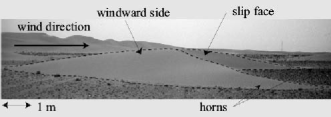
Figure 1: Side view of a barchan dune . The main properties of barchan dunes are outlined: two horns pointing downwind, the slip-face and the flat main body. The barchan shown is approximately $20$ meters long and wide, and $2$ meters high. The slip-face angle is roughly $30^{o}$ to the vertical, which corresponds to the angle of repose of a sand-pile.

A side view of a barchan - see Fig. 1 - shows a rather flat aerodynamic structure. When viewed from above, a barchan presents a crescentic shape with two horns pointing downwind. A sharp edge - the brink line - divides the dune in two areas: the windward side and the slip face, where avalanches develop - see Fig. 2. Because of a boundary layer separation along this sharp edge B41 ; CWG93 ; PT90 , a large eddy develops downwind and wind speed decreases dramatically. Therefore, the incoming blown sand is dropped close to the brink line. That is why the barchan is known to be a very good sand trapper. Sometimes, when the drift of sand is too large, an avalanche occurs and grains are moved down the slip face. In short, grains are dragged by the wind from the windward side of the dune to the bottom of the slip-face and, grain after grain, the dune moves. Field observations show that barchans can move up to $70m/year$ SRPH01 . Their speed is dependent on wind power and on their size: for the same wind strength, the velocity of barchans is roughly inversely proportional to their heights B41 ; ACD01 ; CWG93 ; LL69 ; S90 . Barchan dimensions range from $1$ to $30$ meters high, and from $10$ to $300$ meters long and wide B41 ; CWG93 ; PT90 . However, large barchans are often unstable, leading to complex structures called mega-barchans CWG93 ; PT90 . More accurate analyses reveal that the height, width and length are related by linear relationships ACD01 ; HH98 and that no mature barchan dune smaller than one meter high can be found: there is a minimal barchan size. Finally, the last important characteristic of barchans, but much less well-documented, is the sand leak at the tip of the horns B41 ; CWG93 ; PT90 ; HACHD03 , where no recirculation bubble develops. This shows that barchan dunes are three dimensional structures, whose center part and horns have totally different trapping efficiency - see Fig. 2.

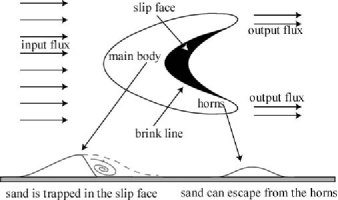
Figure 2: Barchan dune properties. Grains follow the wind direction, and sand flux is not strongly deflected by the dune relief. As observed in the field, sand grains can escape from the horns, but not from the main dune body. Instead, they are trapped into the slip-face. This difference of behavior between the main body and the horns is the key to understand the barchans.

Because of the inherent difficulties of field-work, (a typical mission duration is rather short compared to the lifetime of a dune and its shape movement), numerical modeling is, alongside laboratory experiment HDA02 , an important method to explore barchan properties such as their morphogenesis, their stability and their interaction modes, which are still poorly understood. Obviously, these problems are related to the original structure of barchans, and, accordingly, they should be studied with a $3d$ approach. The aim of the present paper is to discuss how to extend existing $2d$ models to the $3d$ situation. Then, we will show that the crescentic shape can be explained by the existence of a sand-flux constraint and a lateral sand-flux. In the following part, we start by recalling briefly the main features of $2d$ modeling of dunes . Then a model for the $3d$ situation will be presented.

2 The $\mbox{{C}}_{\mbox{{c}}}^{\mbox{{c}}}$ class of models

Numerical modeling of dune requires a description of the effect of wind flow over a sand-bed. Obviously, computing exact turbulent numerical solution starting with the Navier-Stokes equations is possible, but this would take a very long time. An alternative is to use the $\mbox{{C}}_{\mbox{{c}}}^{\mbox{{c}}}$ model ACD02 , based on the following approach.

2.1 Numerical model for the $2d$ case

Let us call $h(x,t)$ the sand bed profile and $q(x,t)$ the vertically integrated volumic sand-flux. They are linked by the mass conservation:

$$\partial_{t}h+\partial_{x}q=0.$$ (1)

The sand flux $q(x,t)$ is the main physical parameter needed to understand dune physics. It cannot locally exceed a saturated value $q_{sat}(x,t)$, which is the maximum number of grains that the wind is able to drag per unit of time at $x$. Previous work have already focused on the important role played by the saturation of the sand flux and the so-called saturation length, $l_{sat}$ HDA02 ; K02 ; ACD02 . The nature of this saturation process can be understood in terms of sand grain inertia: if the wind speed increases, it takes some time for the grains, initially at rest, to reach the wind velocity. Different approaches are possible to describe the evolution of the sand flux towards its saturated value $q_{sat}$. However for the sake of simplicity, this saturation process is here taken into account with the equation,

$$\partial_{x}q=\frac{q_{sat}-q}{l_{sat}}.$$ (2)

This equation keeps the most important effect: the existence of a characteristic length-scale $l_{sat}$. Moreover, $q_{sat}$, depends on the wind shear velocity $u_{*}$. Even if the nature of this dependency is still debated, the saturated flux is a growing function of $u_{*}$ ASW91 ; Sorensen01 ; A03 . Then a linear expansion of $q_{sat}$, as proposed in the innovative work of Sauermann et al. S01 ; K02 from the model of Jackson & Hunt JH75 leads to:

$$\frac{q_{sat}(x)}{Q}=1+A\int\!\!\frac{d\chi}{\chi}\,\partial_{x}h_{e}(x-\chi)+B\,\partial_{x}h_{e}(x),$$ (3)

where $Q$ is the saturated flux value on a flat ground and $h_{e}(x)$ is the envelope of the dune. This envelope encages the dune and its recirculation bubble S90 , and is used to include the boundary layer separation heuristically. Notice that in the latter equation, $h_{e}(x,t)$ appears only through its first spatial derivative. It is consistent with the assumption that atmospheric turbulent boundary layer is fully developed, so changes in $u_{*}$, and accordingly in $q_{sat}$ are scale-invariant. From an aerodynamical point of view, this relation takes into account two effects: a pressure effect, controlled by $A$, where the whole shape acts on the wind flow; and a destabilizing effect, controled by $B$, which ensures that the maximum speed of the flow is reached before the dune summit. Although in principle we could compute the parameters $A$ and $B$, we prefer to consider them as tunable parameters. Finally, avalanches are simply taken into account: if the local slope exceeds a critical value, the sand flux is increased strongly along the steepest slope. We will come back to the description of avalanches in section $4$. The only scaling quantities are $Q$ and $l_{sat}$ and they are used to adimensionalize the problem.

In fact, this model belongs to what we called the $\mbox{{C}}_{\mbox{{c}}}^{\mbox{{c}}}$ class. It does not depend strongly on the model use for the shear stress: other models G02 of shear stress perturbations could be used providing that they include the role of the whole shape ($A$) and the asymmetry of the flow ($B$). The same remarks apply to the charge equationS01 ; K02 and to the equation linking $q_{sat}$ and $u_{*}$. This shows the robustness of the physics ingredients used in this class of model. Even though this method does not provide the most detailed results, this kind of model has been used successfully to model $2d$ barchan profile S01 ; K02 ; ACD02 .

2.2 Speed dispersion and trapping efficiency

As a matter of fact, simulations in $2d$ show the existence of two kinds of solutions: dune and dome ACD02 . The dune solution has a slip-face that catches all the incoming sand: the dune can only grow - except if the input sand flux is null. On the contrary, for a dome, a large amount of sand can escape, and if the loss of sand is not balanced by an influx, the dome can only shrink. Hence, these two solutions cannot co-exist. To compute the steady shape of a $3d$ barchan, it is possible to cut it in ”slices” parallel to the wind direction and, for each slice, to use the $2d$ model to compute its evolution. However, in a real barchan, a $2d$ slice from the horns seems to behave like $2d$ dome solution, while a $2d$ slice from the main body coresponds to $2d$ dune solution. However, in order to make slices from the main body and slices from the horns coexist, we must introduce a sand flux which will redistribuate laterally the sand from the center towards the horns. This sand flux coupling is also needed to overcome the speed dispersion effect. As a matter of fact, if all the slices have initially the same shape - but at a different scale ratio - the saturated flux at the crest is the same for all the slices, as imposed by turbulence scale invariance and the speed of a slice is given by:

$$c=\frac{q_{c}-q_{out}}{h_{c}}$$ (4)

where $q_{c}$ and $q_{out}$ are respectively the flux at the crest and the output flux, and $h_{c}$ is the height at the crest of the slice. Hence, the smaller the slice, the faster its motion. This dispersion explains why the barchan takes a crescentic shape. But to reach a steady state, all the slices must move at the same speed. Therefore, the lateral coupling must also induce a speed homogenization.

3 Different lateral coupling mechanisms

What physical mechanisms can lead to a redistribution of the sand flux on the dune surface? We can think of three different possibilities: avalanches, lateral wind shear stress perturbations and grain motions (saltation and/or reptation).

3.1 Avalanches

First, avalanches develop in three dimensions along the steepest slope. This creates lateral sand flux in the slip face area. However, for real barchan dunes, that sand-transport is directed from the edges towards the center. Accordingly, the center part grows and slows down while the border slices shrink and accelerates. This does not constitute a stabilizing mechanism.

3.2 Wind deflection

The lateral wind deflection is another possibility. Field observations B41 and numerical simulations S01 tend to show that, due to its flatness, the dune does not make the wind flow deviate too much laterally. Consequently trajectories of grains are not dragged into the lateral direction. Nevertheless, it is always possible to compute the wind speed perturbations in the lateral direction and see what it gives. This has been done recently SH03-2 , but there is hardly any evidence that it is the main physical process responsible for a lateral sand flux on the dune. On the other hand, it appears to be an important effect for the development of lateral instabilities along transversal dunes SH03-1 .

3.3 Saltation and reptation coupling

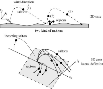
Figure 3: Influence of gravity. While trajectories of saltons are deflected randomly at each collision, the reptons are always pushed down along the steepest slope.

A better candidate is the grain motion. Sand transportation can be described in terms of two species A03 : grains in saltation - the saltons - and grains in reptation - the reptons - see Fig. 3. Saltons are dragged by wind, collide with the dune surface, rebound, are accelerated again by the airflow, and so forth. At each collision, saltons dislodge many reptons, which travel on a short distance, rolling down the steepest slope, and then, wait for another salton impact.

As the wind deflection is weak, we assume that saltons follow quasi $2d$ trajectory in a vertical plane (see last section), except when they collide with the dune. At each collision, they can rebound in many directions, depending on the local surface properties, and this induces a lateral sand flux. Given that the deflection by collision is strongly dependent on the surface roughness, we assume that, on average, the deflection of saltons is smaller than for reptons, which are always driven towards the steepest slope. In the following derivation, we will neglect the sand flux deflection due to saltation collisions.

Despite the major role played by saltons in dune dynamics, the presence of reptons should not be dismissed. According to field observations HW88 ; H77 , reptons are strongly dependent on the local slope: this can be observed by looking at the relative orientation of the wind and ripples. On hard ground, ripples are perpendicular to wind direction, but on a dune their relative orientations change with the local slope H77 . Even if one is reluctant to use the saltation coupling because of its inherent difficulties, the reptons would still be rolling on the dune surface: gravity naturally tends to move the grains along the steepest slope, leading to lateral coupling of the dune slices. In the following part, we will focus on this coupling by reptation, which has never been used for the study of barchan dunes. The saltation process remains important in this model, since it induces reptation coupling.

4 A $3d$ model with reptation coupling

4.1 Formulation of the model

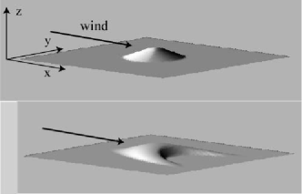
Figure 4: Typical initial and final shape of barchan dunes given by the $3d$ $\mbox{{C}}_{\mbox{{c}}}^{\mbox{{c}}}$ model. Parameters used are $A=9.0$, $B=5.0$, $D=0.5$ with initially: $W_{0}=30l_{sat}$, $H_{0}=3l_{sat}$.

As reptons are created by saltons impacts, the part of the flux due to reptons is assumed to be proportional to the saltation flux, $q_{sal}$ B41 . Hence, the flux of reptons is simply written as discussion :

$$\vec{q_{rep}}=\alpha q_{sal}(\vec{e_{x}}-\beta\vec{\nabla}h)$$ (5)

The $\alpha$ coefficient represents the fraction of the total sand flux due to reptation on a flat bed. In case the bed is not flat, the flux is corrected to the first order of the $h$ derivatives, by a coefficient $\beta$ and directed along the steepest slope to take into account the deflection of reptons trajectories by gravity. Assuming that saltation trajectories are $2d$, the total sand flux $\vec{q}$ is given by:

$$\vec{q}=q_{sal}(1+\alpha)\vec{e_{x}}-\beta\alpha q_{sal}\vec{\nabla}h$$ (6)

Moreover, reptation flux is assumed to instantaneously follow the saltation flux, so that there is no other charge equation than the saltation flux one:

$$\partial_{x}q_{sal}=\frac{q_{sat}-q_{sal}}{l_{sat}}.$$ (7)

Then, the mass conservation equation becomes:

$$\partial_{t}h+\partial_{x}q_{sal}+\vec{\nabla}\vec{q_{rep}}=0.$$ (8)

Calling $D=\alpha\beta/(1+\alpha)$ and $\tilde{q}=(1+\alpha)q_{sal}$, the two latter equations can be rewritten as :

$$\partial_{x}\tilde{q}=\frac{\tilde{q}_{sat}-\tilde{q}}{l_{sat}}$$ (9)

$$\partial_{t}h+\partial_{x}\tilde{q}=D(\partial_{x}(\tilde{q}\partial_{x}h)+\partial_{y}(\tilde{q}\partial_{y}h))$$ (10)

Finally, we obtain the same set of equations as in the $2d$ $\mbox{{C}}_{\mbox{{c}}}^{\mbox{{c}}}$ model, but with one more phenomenological parameter, $D$, which can be understood as the importance of the lateral coupling, because of lateral deflection of reptons. This formulation appears to be a nonlinear difusion equation driven by the non dimensionnal coefficient $D$. For a homogeneous flux solution, $QD$ appears to be a diffusion coefficient, showing the diffusion-like role of the coupling coefficient $D$. Notice that $\tilde{q}$ is no longer the saltation flux, but the part of the flux that does not depend on the bed slope. Avalanches are computed in three dimensions using a simple trick. If the local slope exceeds the threshold $\mu_{d}$, the sand flux is strongly increased by adding an extra avalanche flux:

$$\vec{q_{a}}=E(\delta\mu)\vec{\nabla}h,$$ (11)

where $\delta\mu$ is null when the slope is lower than $\mu_{d}$ and equal to ($\delta\mu=|\vec{\nabla}h|^{2}-\mu_{d}^{2}$) otherwise. For a sufficiently large coefficient $E$, the slope is relaxed independently of $E$. Finally, note that quasi-periodic boundary conditions (the total output flux is reinjected homogeneously in the numerical box) are used to perform the numerical simulations. These boundary conditions are used, first to work with a constant mass, and second to force the system to converge towards its steady state. Obviously these boundary conditions constrain the final shape.

4.2 The origins of the crescentic shape

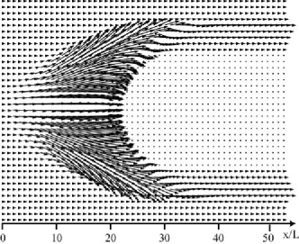
Figure 5: Lateral diffusion of sand flux. The angle of the flux vectors are magnified $3$ times to be clearly visible. Both the deflection towards the horns and the presence of avalanches can be observed. Parameters used are the same than for figure 4 and 6: $A=9.0$,$B=5.0$,$D=0.5$ with initially: $W_{0}=30l_{sat}$, $H_{0}=3l_{sat}$.

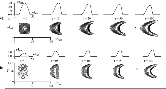
Figure 6: Barchan formation. a) evolution of an initial cosine bump sand pile : $h(x,y)=\cos(2\pi x/W_{0})\cos(2\pi y/W_{0})$. In the beginning, the horns moves faster than the central part of the dune, leading to the formation of the crescentic shape. The shape reaches an equilibrium thanks to the lateral sand flux, which feeds the horns. Parameters used are the same than for figures 4 and 5: $A=9.0$,$B=5.0$,$D=0.5$ with initially: $W_{0}=30l_{sat}$, $H_{0}=3l_{sat}$. b) Evolution of a bi-cone sand-pile (same parameters than in (a)). This shows that emergence of a crescentic shape is independant on initial shape: the hole in the middle is filled up, and a crescentic shape forms. In both boxes the height between two level-lines is $0.2l_{sat}$.

Our $3d$ $\mbox{{C}}_{\mbox{{c}}}^{\mbox{{c}}}$ model depends on three phenomenological parameters : $A$ and $B$ take into account aerodynamics effects, and $D$ describes the efficiency of the slices coupling. The final shape, if one exists, depends on these parameters. For example, Fig. 4 shows a typical $3d$ final steady state of a computed barchan dune, which looks likes a real aeolian one. The arrows on Fig. 5 indicate the direction of the total sand flux on the whole dune shape. The deviation towards the horns is clearly visible as the sand captured by the slip-face. Looking at Fig 6 helps us to understand the formation of the crescentic shape of barchan dune. Starting from a sand-pile, some horns will appear and since they are faster than the center slice of the dune, a crescentic shape appears. Now, let us consider a slice and let us call $q_{x}$, the excess flux due to reptons coming from the lateral sand flux, $q_{in}$ the incoming saltation sand flux brought by the wind and $q_{e}$ the flux due to erosion. The existence of a saturated flux imposes :

$$q_{e}+q_{x}+q_{in}<q_{sat}^{max}.$$ (12)

where $q_{sat}^{max}$ is the maximum value of the saturated flux on the given slice. Thus, if the excess flux $q_{x}$ increases, the erosion flux, $q_{e}$, decreases. As the speed of the slice is governed by the erosion, the slice slows down. After a while, the horns receive enough sand from the main body to decrease their speed and to compensate the output flux. Finally the speed of all slices is the same and the barchan moves without changing its shape. Moreover, the center part, which would grow without lateral coupling, can now have an equilibrium shape, since all the extra flux is deviated towards the horns. Furthermore this coupling process is stabilizing with respect to local deformation. If a slice increases in height, the excess sand flux leaving the slice will increase, and the deformation will shrink. Similarly, starting from a two maxima shape, the part of the flux sensitive to the local slope tends to fill up the gap between the two maxima: the whole mass is redistributed and a single barchan shape is finally obtained - see Fig. 6. This agrees with the apparent robustness of the crescentic shape observed on the field. Whatever the external conditions are, the same morphology is roughly found everywhere where barchans develop. Hence, this lateral coupling helps us to understand such barchan structures. However, we have no clue about the possible value of this coupling coefficient $D$ and it is therefore useful to study the influence of $D$ on the barchanic shape.

5 Significance of the coefficients

5.1 The influence of the coupling coefficient $D$

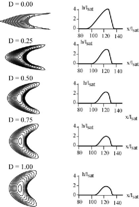
Figure 7: Different $3d$ shapes obtained for different values of $D$ and for the same initial sand-pile. Parameters used (except for $D$ coefficient) are the same than for figures 4, 5 and 6. Computations are performed with quasi-periodic boundary conditions. The barchan central slice is represented on the right. Notice that for $D=0$, a steady state is reached because of lateral sand redistribution due to avalanches on the windward side. However, there is a sharp edge which separates the dune in two part, leading to an arrow shape rather than to a crescentic shape.

As can be seen on Fig. 7, $D$ has a crucial influence on the global morphology. First of all, for a small $D$, (i.e. a small lateral sand flux), the flux escaping from the tip of the horns is mainly due to $q_{in}$ and to the erosion flux, $q_{e}$. Therefore, erosion may be important, and the horns may move quickly. Thus, during the transient, the barchan elongates. On the contrary, for a larger $D$, the lateral flux received by the horns, $q_{x}$, is larger and then the erosion is less important. The horns move slower and the elongation is shorter.

Secondly, the width of the horns is also dependent on $D$. For a large $D$, the deflected flux is large. However, as the output sand flux cannot exceed a maximum value, horns have to be wide in order to transport away all the incoming sand, and indeed, the width of the horns increases with $D$. This simple explanation is confirmed by numerical simulation, as depicted in Fig. 7 and Fig. 8. Measuring the width of the horns in the desert may be a convenient way to estimate the value of $D$ from field observations.

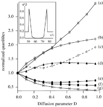
Figure 8: Dependance of barchan dune properties on the coupling coefficient $D$. The case with $D=0$ is taken has a reference. The properties are: (a) width of a horn, (b) total width, (c) equilibrium input flux, (d) speed of the dune , (e) total length (including horns), (f) length of the center slice, (g) maximum height. A typical output flux cross section is shown in the upper left part of the graph: the width of the horns is measured by measuring the width of the flux peaks. The initial sand pile is always a cosine bump defined by $h(x,y)=H_{0}\cos(2\pi x/W_{0})\cos(2\pi y/W_{0})$ with $W_{0}=20$ and $H_{0}=2.0$.

Finally the aspect ratio of the dune, $h/w$, varies with $D$, because the coupling mechanism tends to diminish slopes. In other words, the dune tends to spread out laterally when $D$ increases, sometimes leading to structures without a slip-face: $3d$ dome solution. In this case, sand can escape from the whole transversal section of the dune and the output flux is then higher than for the dune solution. Basically the transition from $3d$ dune to $3d$ dome situations occurs when the horn width is equal to half the dune width. This corresponds approximately to $D=2.0$ with the parameters $A=9.0$ and $B=5.0$. For too large a diffusion, the dune becomes very wide and flat, without a slip-face, and remains unsteady.

5.2 The influence of coefficients $A$ and $B$

However, looking only at the $D$ influence is not accurate enough to describe qualitatively the influence of diffusion. In fact, the shape is the result of three physical effects governed by the parameters $A$, $B$ and $D$. Fig. 9 presents a phase diagram with $D$ kept constant at a value of $0.5$. Many different morphologies can be observed, from a large and thin unsteady crescent to a flat unsteady sand patch, and with steady barchans inbetween. First, $A$ governs the stability of the sand bed, and then a large $A$ tends to flatten the sand-pile. Increasing $B$, on the other hand, forces the slope to increase and to nucleate a slip-face. Thus, when the ratio $A/B$ is high, there is hardly a slip face. On the contrary, when it is low, the slip face develops on the whole dune. Thus the $A/B$ parameter controls the way the slip-face appears. Secondly, one can observe that the dunes obtained with a constant ratio $A/B$ have different morphologies. This shows that for small $A$ and $B$ the coupling coefficient $D$ plays an important role in the shaping of the dune. Field measurements of the horns’ width and the minimal size of barchans should help us to give an estimation of these parameters. The following table provides with a summary of the different qualitative effects of $A$,$B$ and $D$.

	physical mechanism	Main effect when increasing
$A$	curvature effect	$L$ increases,
		$W$ decreases.
$B$	slope effect	Slip-face appears easily,
		$\partial_{x}h$ increases, $W$ increases.
$D$	Lateral coupling	$H$ decreases,
		$W$ and horns width increase,
		output flux increases.

Finally, the initial sand-pile does not always reach a constant shape. For large $A/B$ no steady state appears. This is due to the fact that the erosion is so strong that it cannot be balanced by the influx, and the sand-pile just becomes flatter and flatter. On the contrary, for a large $B/A$, a thin unsteady crescent appears. Finally, for a large $D$ (compared to $A$ and $B$) steady and unsteady dome solutions are produced by the numerical model. This shows the importance of $A$, $B$ and $D$ on the shape and on the minimal size of computed barchan dunes.

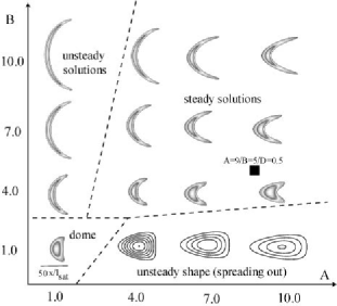
Figure 9: Evolution of the same initial cosine bump sand pile ($h(x,y)=\cos(2\pi x/W_{0})\cos(2\pi y/W_{0})$ with $W_{0}=30l_{sat}$, $H_{0}=3l_{sat}$) changing the value of the parameters $A$ and $B$. $D$ is kept constant and equal to $0.5$. The dashed lines separate qualitatively the different stability and shape domains. The dome domain is divided into two parts depending on the steadiness of the dome solution.

6 Conclusion

We have seen that reptation can be used to describe the $3d$ crescentic shape of barchan dunes. As reptons are sensitive on the local slope, they induce a lateral sand flux. This allows a given sand-pile blown by the wind to reach an equilibrium shape, despite varying ”slices” speed and intrinsic differences between the main body and the horns. The crescentic shape comes from two mechanisms, which compete with each other. The first one is the speed dispersion within the dune: the small height slices are faster than higher ones, leading to the crescentic shape, and eventually to the destruction of the barchan dune. The second one, is the lateral flux deflection that reduces the horns’ speed by decreasing the erosion flux on them. It leads to the homogenization of the speed of the different slices, and eventually to the propagation of a steady state dune or a steady sand dome. This mechanism is efficient since the overall excess flux can escape from the horns. In other words, barchanic shape appears to be the very basic shape taken by any sand-pile blown by a unidirectional wind. Now that the steady shape of barchan dunes seems to be well described, it would be interesting to study the dynamics of such a structure placed far from equilibrium conditions, because, in the field, input flux has no reason to be related to the output flux of a dune.

As a matter of fact, in this paper, barchans have been numerically obtained with quasi-periodic boundary conditions. If standard boundary conditions are used, a typical barchan dune takes the crescentic shape, for the same reasons as the ones exposed in this article, but it keeps growing or shrinking depending on the incident sand flux, either higher or lower than the sand flux escaping from the hornsHACHD03 . This point is crucial because it suggests that single real barchan dunes are not steady structures and, moreover, it shows that a crescentic shape can form even if the dune is not in an equilibrium state. Therefore, further investigations are still required to understand the long-term existence and shape of barchan dune in the field. In our model we have neglected saltation coupling; but we believe that it is not the dominant effect. Moreover, it could easily be taken into account by adding a new coupling coefficient dedicated to lateral deflection of saltons.

Finally, it appears that depending on the coupling coefficient, $D$, the solution can either be a $3d$ dome or a $3d$ barchan. Similarly, changing $A$ and $B$ can lead to different shapes, and different behavior. it might be interesting to understand the transformation of a $3d$ sand patch, steady or unsteady, into a barchan dune because of fluctuations of these parameters, and particularly of $D$ variations. As a matter of fact, these parameters may depend on external conditions such as grains size distribution, humidity or wind fluctuation.

Acknowledgement : The author is grateful to T. Bohr for his constructive remarks. The author whishes to thank K.H. Andersen, B. Andreotti, P. Claudin and S. Douady for their important role in this work, and also S. Bohn for delightful discussions about barchans. This work has benefited from an ACI J.Ch.

References

- (1) R.A. Bagnold.The physics of blown sand and desert dunes. Chapman and Hall, London, 1941.
- (2) B. Andreotti, P. Claudin, S. Douady. Selection of dune shapes and velocities. part 1: Dynamics of sand, wind and barchans. Eur. Phys. J. B, 38, 341-352, (2002).
- (3) P. Hersen, S. Douady, B. Andreotti. Relevant length scales for barchan dunes. Phys. Rev. Lett., 264301, (2002).
- (4) R. Cooke, A. Warren, A. Goudie. Desert Geomorphology. UCL press, 1993.
- (5) K. Pye, H.Tsoar. Aeolian Sand and sand dunes. Unwin Hyman, London, 1990.
- (6) H.J. Finkel. The barchans of southern Peru. J. Geol., 67, 614-647 , (1959).
- (7) J.T. Long, R.P. Sharp. Barchan dune movement in imperial valley, california. Geological Society of America Bulletin, 75, 149-156, (1964).
- (8) R.M. Norris, Barchan dune of imperial valley, California, J. Geol., 74, 292-306, (1966).
- (9) S.L. Hastenrath. The barchans of the arequipa region, southern peru. Zeitschrift für Geomorphologie, 11, 300-331, (1967).
- (10) K. Lettau, H.H. Lettau. Bulk transport of sand by the barchans of La Pampa La Hoja in southern Peru. Zeitschrift für Geomorphologie 13, 182-195 (1969).
- (11) S. Hastenrath. The barchan dunes of southern peru revisited. Z. Geomorph. N. F, 31 (2), 167-178, (1987).
- (12) M.C. Slattery. Barchan migration on the Kuiseb river delta, Namibia. South African Geographical Journal, 72, 5-10 (1990).
- (13) P.A. Hesp, K. Hastings. Width, height and slope relationships and aerodynamic maintenance of barchans. Geomorphology, 22, 193-204, (1998).
- (14) G. Sauermann, P. Rognon, A. Poliakov, H.J. Herrmann. The shape of the barchan dunes of southern morocco. Geomorphology, 36,47-62, (2000).
- (15) F.K. Wippermann, G. Gross. The wind-induced shaping and migration of an isolated dune : a numerical experiment. Boundary-Layer Meteorology, 36, 319-334, (1986).
- (16) H. Nishimori, N. Ouchi. Formation of ripple patterns and dunes by wind-blown sand. Phys. Rev. Lett., 71 (1), 197-200, (1993).
- (17) B.T. Werner. Eolian dunes : Computer simulations and attractor interpretation. Geology, 23 (12), 1107-1110, (1995).
- (18) H. Nishimori, M. Yamasaki, K.H. Andersen. A simple model for the various pattern dynamics of dunes. J. Mod. Phys., B12, 256-272, (1997).
- (19) J.M.T. Stam. On the modelling of two dimensional aeolian dunes. Sedimentology, 44, 127-141, (1997).
- (20) J.H. van Boxel, S.M. Arens, P.M. van Dijk, Aeolian processes across transverse dunes. I: Modelling the air flow, Earth Surface Processes and Landforms, 24, 255-270, (1999).
- (21) G. Sauermann. Modeling of Wind Blown Sand and Desert Dunes. PhD thesis, Universitat Stuttgart, (2001).
- (22) K. Kroy. Minimal model for Aeolian sand dunes, Phys. Rev. E, vol 66, 031302, (2002).
- (23) B. Andreotti, P. Claudin, S. Douady. Selection of dune shapes and velocities. part 2: A two-dimensional modelling. Eur. Phys. J. B, 28, 321-339, (2002).
- (24) P. Hersen, K.H. Andersen, H. Elbelrhiti, B. Andreotti, P. Claudin, S. Douady, Corridors of barchan dunes: stability and size selection. to appear in Phys. Rev. E, (2003).
- (25) R.S. Anderson, M. Sørensen, B.B. Willetts. A review of recent progress in our understanding of aeolian transport. Acta Mechanica [suppl], 1, 1-19, (1991).
- (26) M. Sørensen. On the rate of aeolian sand transport. Atelier international : Formation et migration des Dunes, Nouakchott, 2001.
- (27) B. Andreotti. A two species model of aeolian sand transport. to appear in J. Fluid. Mech. (2003).
- (28) P.S. Jackson and J.C.R. Hunt, Turbulent wind flow over a low hill, Quart. J. R. Met. Soc. 101, 929-955 (1975).
- (29) A.C. Fowler. Geomorphological Fluid Mechanics, chapter 16, 430-454. Springer-Verlag, Berlin, 2001.
- (30) V. Schwammle, H.J. Herrmann. A model of barchan dunes including lateral shear stress. cond-mat/0305036, (2003).
- (31) V. Schwammle, H.J. Herrmann. Modeling transverse dunes cond-mat/0301589, (2003).
- (32) J. Hardisty, R.J.S. Whitehouse. Evidence for a new sand transport process from experiments on sahara dunes. Nature, 332, 532-534, (1988).
- (33) A.D. Howard. Effect of slope on the threshold of motion and its application to orientation of wind ripples. Geological Society of America Bull. 88, 853-856, (1977).
- (34) K.H. Andersen, B. Andreotti, P. Claudin. private communication, (2002/2003).
- (35) These boundary conditions induces also a weak coupling between slices: the output flux is not homogeneous, so a part of the sand escaping from the horns is transfered to the center of the dune.