Population Coding by Globally Coupled Phase Oscillators

Abstract

A system of globally coupled phase oscillators subject to an external input is considered as a simple model of neural circuits coding external stimulus. The information coding efficiency of the system in its asynchronous state is quantified using Fisher information. The effect of coupling and noise on the information coding efficiency in the stationary state is analyzed. The relaxation process of the system after the presentation of an external input is also studied. It is found that the information coding efficiency exhibits a large transient increase before the system relaxes to the final stationary state.

1 Introduction

Oscillatory activity of neurons is ubiquitous in various areas of the brain at various scales, whose physiological relevance to the information processing has been discussed in a number of studies [1, 2, 3, 4]. In modeling cortical neural circuits, coupled oscillators have played important roles [5, 6]. In this framework, the neurons are modeled as mutually interacting limit-cycle oscillators, where simplified interaction rules between the oscillators are often assumed for the sake of mathematical tractability. The case of global (all-to-all) coupling is typical of such simplified interactions, where the oscillators interact through the mean field of all oscillators. The prominent feature of globally coupled oscillators is complete synchronization [5, 7, 8, 9]. However, it is experimentally known that the cortical neurons in vivo rarely exhibit large-scale complete synchronization, but usually exhibit irregular firing patterns [10]. Therefore, it has been discussed how globally coupled models of neural populations can sustain asynchronous firing activity [11, 12, 13, 14, 16, 15].

It is generally considered that the cortical information processing is achieved through population coding, namely, collective representation of information by large numbers of neurons [17, 18, 19]. Regarding quantification of information coding efficiency by a population of neurons, a framework based on statistical estimation theory has been utilized. In this framework, the information coding efficiency is quantified by how precisely the given stimulus can be estimated from the observed firing rates of those neurons. It can be measured by the Fisher information, which gives the accuracy of parameter estimation in statistical estimation theory [20, 21]. Using this framework, the information coding efficiency of various stochastic neuron models has been calculated [17, 18, 19].

In this paper, instead of stochastic neuron models, we introduce a system of globally coupled phase oscillators as a simple model of cortical neural circuits. Our system exhibits asynchronous state where each oscillator rotates (“fires”) independently, by which we model the “irregular firing” of the cortical neurons. It codes the parameter value of an external input in the asynchronous phase distribution of the oscillators. We quantify the information coding efficiency of our system using the statistical estimation framework. We discuss the effect of coupling and noise on the information coding efficiency in the asynchronous stationary state. We also study the dynamical aspect of our system. Even if the oscillators are not in strict synchrony with each other, their population density can still exhibit coherent damped oscillation. We show that such oscillation can lead to a large transient increase in the information coding efficiency.

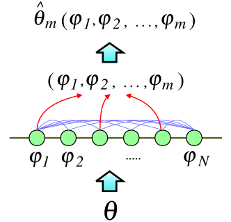
Figure 1: Population coding by globally coupled phase oscillators. Information coding efficiency of the system is quantified using Fisher information, which gives the accuracy of an estimator $\hat{\theta}_{m}(\varphi_{1},...,\varphi_{m})$ of the external input parameter $\theta$ from observed phase variables $\varphi$ of the oscillators.

2 Globally coupled phase oscillators

We use a system of globally coupled phase oscillators, which was previously studied in detail by Golomb et al. [5]. It exhibits asynchronous states as well as various synchronized states. We set the system at its asynchronous state, and add a constant external input to the system that depends on a given external parameter $\theta$. This parameter $\theta$ is then coded by the non-uniform phase distribution of the oscillators (Fig. 1). Our interest is how efficiently the population of the oscillators codes this external parameter. We quantify it by how precisely we can estimate the given input by observing the phase variables of the oscillators. This system may be considered, for example, as a simple qualitative model of the orientation column in the visual cortex [17, 18, 16, 15]. In that case, the external parameter $\theta$ corresponds to the angle of a visual directional stimulus.

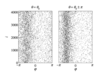
Figure 2: Snapshots of the phase $\varphi$ of the oscillators at two values of the external input, $\theta=\theta_{0}$ and $\theta=\theta_{0}\pm\pi$.

Our system consists of $N$ identical phase oscillators mutually interacting through their mean field, which obey the following Langevin equations:

$$\frac{d}{dt}\varphi_{i}(t)=f(\varphi_{i}(t))+\frac{1}{N}\sum_{j=1}^{N}g(\varphi_{j}(t))+\xi_{i}(t)+H(\theta)$$ (1)

for $i=1,...,N$, where $\varphi_{i}$ represents the phase of the $i$-th oscillator, $f(\varphi)=A+\sin\varphi$ the individual dynamics of an isolated oscillator, $g(\varphi)=C\sin(\varphi+\alpha)$ the interaction between the oscillators, and $\xi_{i}$ a Gaussian-white noise with zero mean, whose correlation function is given by $\langle\xi_{i}(t)\xi_{j}(t^{\prime})\rangle=2D\delta(t-t^{\prime})\delta_{i,j}$. We identify $\varphi+2\pi k$ ($k$ is an integer number) with $\varphi$ and restrict the value of $\varphi$ in $[-\pi,\pi]$. $H(\theta)$ is a $\theta$-dependent constant external input common to all oscillators, which we explain below. The parameter $A$ determines the dynamics of each oscillator, $C$ the coupling strength, $\alpha$ the phase shift of coupling, and $D$ the intensity of noise. We assume that $C$ can take both positive and negative values, and the range of $\alpha$ to be $(0,\pi)$. We exclude two extreme values $\alpha=0$ and $\alpha=\pi$, since the system becomes singular with these values [5].

When isolated, each oscillator exhibits both excitatory and self-oscillatory dynamics depending on the value of $A$ (without the noise and the external input, each oscillator is self-oscillatory when $A>1$). To realize the asynchronous state, we set $A$ at a sufficiently large value, so that each oscillator is self-oscillatory even if the effects of the coupling, the noise, and the external input are incorporated. In this self-oscillatory situation, the mean rotation rate (or the “firing rate”) of the oscillator increases with $A$.

Through the external input $H(\theta)$, the dynamics of the phase $\varphi$ is affected by the external parameter $\theta$. We assume the range of $\theta$ to be $[-\pi,\pi]$ (“angle stimulus”) and use a functional form $H(\theta)=H_{0}\cos(\theta-\theta_{0})$ as the external input, where $H_{0}$ determines its strength and $\theta_{0}$ the location of its maximum (“preferred stimulus”). This $H(\theta)$ roughly models the one-humped “tuning curve”, which represents the response of a neuron to the stimulus [17, 18, 19]. When $\theta$ approaches $\theta_{0}$, the mean rotation rate of the oscillators increases, and reaches the maximum value at $\theta=\theta_{0}$ (in the following discussion, the results depends only on the difference $\theta-\theta_{0}$, so that the absolute value of $\theta_{0}$ is not important). Since this external input $H(\theta)$ merely shifts the parameter $A$ in the individual dynamics of the oscillator $f(\varphi)=A+\sin\varphi$, we hereafter include $H(\theta)$ in $A$ and denote the effective value of $A$ as $A(\theta)=A+H(\theta)$.

Figure 2 displays two snapshots of the phase $\varphi_{i}$ of all oscillators in the asynchronous stationary state obtained by direct numerical simulations of the Langevin equations (1) at two different values of the external input, $\theta=\theta_{0}$ and $\theta=\theta_{0}\pm\pi$ ($\theta=\theta_{0}+\pi$ and $\theta_{0}-\pi$ give the same external input because $H(\theta)$ is periodic in $\theta$). The other parameters are fixed at $A=1.5$, $C=0.5$, $\alpha=\pi/4$, $H_{0}=0.1$, and $D=0.1$. It can be seen that the distribution of the phase is relatively uniform at the preferred input $\theta=\theta_{0}$, whereas its non-uniformity is enhanced at $\theta=\theta_{0}\pm\pi$.

Hereafter, rather than tracking the individual stochastic trajectories of the oscillators directly, we take the $N\to\infty$ limit and consider the one-body probability density function (PDF) $P(\varphi,t;\theta)$ of the phase $\varphi$. The evolution of the PDF $P(\varphi,t;\theta)$ is described by [5, 7, 8]

$$\frac{\partial}{\partial t}P(\varphi,t;\theta) = -\frac{\partial}{\partial\varphi}I(\varphi,t;\theta),$$ (2)

$$I(\varphi,t;\theta) = \left\{A(\theta)+G(t;\theta)+\sin\varphi\right\}P(\varphi,t;\theta)$$ (6)

$$-D\frac{\partial}{\partial\varphi}P(\varphi,t;\theta),$$

where $I(\varphi,t;\theta)$ represents the probability flux, and $G(t;\theta)$ the “internal field” defined as the interaction function averaged by the PDF $P(\varphi,t;\theta)$, i.e.,

$$G(t;\theta)=\int_{-\pi}^{\pi}P(\varphi,t;\theta)C\sin(\varphi+\alpha)d\varphi.$$ (7)

Periodic boundary conditions are assumed for $P(\varphi,t;\theta)$ and $I(\varphi,t;\theta)$ at $\varphi=\pm\pi$.

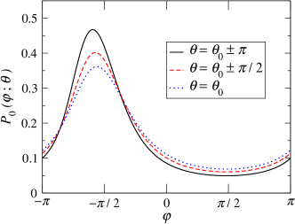
Figure 3: Stationary PDF $P_{0}(\varphi;\theta)$ at several values of the external parameter $\theta$ ($\theta=\theta_{0}\pm\pi$, $\theta=\theta_{0}\pm\pi/2$, and $\theta=\theta_{0}$).

Figure 3 displays stationary PDFs of the phase $P_{0}(\varphi;\theta)$ at several values of the external parameter $\theta$ in the asynchronous stationary state, which corresponds to Fig. 2. The details of this state will be given in the next section. The PDF is relatively uniform at the preferred input $\theta=\theta_{0}$, and becomes steeper at $\theta=\theta_{0}\pm\pi$. At this weak noise level, $D=0.1$, functional shape of the PDF is close to that in the noiseless case. As the value of $\theta$ is varied, the shape of $P_{0}(\varphi;\theta)$ varies correspondingly. In other words, the external parameter $\theta$ is coded by the stationary PDF in the asynchronous state of our globally coupled phase oscillators.

3 Asynchronous stationary state

In this section, we summarize the dynamics of Eqs. (2) and (7) following Golomb et al. [5] with emphasis on the asynchronous stationary state. The PDF $P(\varphi,t;\theta)$ exhibits mainly three behavior, namely, fixed state, limit-cycle state, and asynchronous stationary state. The probability flux $I(\varphi,t;\theta)$ takes a small value in the fixed state (zero in the noiseless case), a non-zero constant value in the asynchronous stationary state, and oscillates periodically in the limit-cycle state.

Let us consider the noiseless case ($D=0$) first. In this case, existence and linear stability of each state can be studied analytically [5]. Here, it should be noted that even if we set $D=0$, we always assume that the system is subject to infinitesimally weak noise, to avoid singular behavior specific to the noiseless equation and to ensure the existence of final steady states [8]. With this understanding, we formally set $D=0$ to facilitate analytical treatment, and compare the analytical results with the numerical simulations at finite values of $D$.

The fixed-state solutions exist when $C^{2}+2C\cos\alpha+1>A(\theta)^{2}$, and the stability conditions are given by $C\cos\alpha>-1+A(\theta)$ or by $C\cos\alpha>-1-A(\theta)$ and $C>0$. In this state, all oscillators take the same fixed phase homogeneously, and the PDF is simply a $\delta$-function with fixed location. The probability flux is constantly zero. The limit-cycle solution exists when $C^{2}+2C\cos\alpha+1<A(\theta)^{2}$, and is stable when $C>0$. In this state, the oscillators exhibit completely synchronized rotation. The PDF is again a $\delta$-function, whose location rotates steadily. The temporal sequence of the probability flux is given by periodically aligned $\delta$-functions.

In our context, these two states are inappropriate for modeling the dynamics of cortical neurons. In the fixed state, all oscillators are trapped to the same fixed phase and never rotate, namely, the neurons do not fire at all. On the other hand, the limit-cycle state corresponds to the completely synchronized firing of all neurons, which is experimentally unrealistic. These situations are not changed even if weak noise is introduced. Only with sufficiently strong noise, these states may be utilized in modeling the dynamics of cortical neurons, but we do not consider such cases in this paper for simplicity.

The asynchronous stationary solution exists when $-\infty<C\cos\alpha<[A(\theta)^{2}-1]/2$. It coexists with the limit-cycle or fixed solution. Unlike the above two cases, the PDF takes a broad functional form in this state. The oscillators are not in synchrony with each other, and rotate with a finite constant rate steadily. The probability flux $I(\phi,t;\theta)$ takes a constant value, which is typically between $0.05$ and $0.20$ at the parameter values we use in this paper. The stationary PDF $P_{0}(\varphi;\theta)$ in the asynchronous stationary state at $D=0$ can be obtained from Eqs. (2) and (7) as

$$P_{0}(\varphi;\theta)=\frac{\left[F(\theta)^{2}-1\right]^{\frac{1}{2}}}{2\pi}\frac{1}{F(\theta)+\sin\varphi}.$$ (8)

Here, $F(\theta)$ is defined as $F(\theta)=A(\theta)+G_{0}(\theta)$, where $G_{0}(\theta)$ denotes the internal field in this stationary state. The value of $G_{0}(\theta)$, or equivalently the value of $F(\theta)$, is determined self-consistently so that $G_{0}(\theta)$ and $P_{0}(\varphi;\theta)$ satisfy Eq. (7). It is explicitly calculated as

$$F(\theta) = \frac{1}{1+2C\cos\alpha}\{(1+C\cos\alpha)A(\theta)$$ (9)

$$\pm \sqrt{(C\cos\alpha)^{2}[A(\theta)^{2}-(1+2C\cos\alpha)]}\}.$$ (11)

When $C=0$ or $\alpha=\pi/2$ ($C\cos\alpha=0$), we obtain a trivial solution $F(\theta)=A(\theta)$, i.e., $G_{0}(\theta)=0$. The relevant solution for $C\cos\alpha\neq 0$ is given by the negative branch when $-\infty<C\cos\alpha<0$, and by the positive branch when $0<C\cos\alpha<[A(\theta)^{2}-1]/2$. When $C\cos\alpha>[A(\theta)^{2}-1]/2$, no stationary PDF exists that corresponds to the asynchronous stationary state.

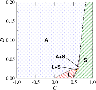
Figure 4: Phase diagram of the system at $A=1.4$. Region “A” represents the asynchronous stationary state, “L” the limit-cycle state, and “S” the fixed state. In the small region “A+S”, the asynchronous state and the fixed state are bistable, and in the region “L+S”, the limit-cycle state and the fixed state are bistable. The dotted curve distinguishes the regions “A” and “S” as defined in the text.

For example, when $0<\alpha<\pi/2$, the non-uniformity of $P_{0}(\varphi;\theta)$ is enhanced as we increase $C$, because $F(\theta)$ decreases. However, as we increase $C$ further, $C\cos\alpha$ eventually reaches $[A(\theta)^{2}-1]/2$, and the stationary PDF corresponding to the asynchronous stationary state ceases to exist. We are then left with a $\delta$-peaked stationary PDF that corresponds to the fixed state of the oscillators.

According to the linear stability analysis of the stationary PDF [5], $P_{0}(\varphi;\theta)$ is marginally stable when $C<0$, and is unstable when $C>0$ in the absence of noise. Therefore, when $C>0$, the asynchronous stationary state cannot be realized without noise, and only the fixed or limit-cycle state is observed in numerical simulations.

When the noise exists ($D>0$), the functional form of the stationary PDF becomes complex. However, we can still obtain it numerically by finding the stationary solution of Eqs. (2) and (7). The $\delta$-peaked PDF in the fixed or limit-cycle state at $D=0$ is smeared by the noise, and takes broader functional form. The asynchronous stationary state is also broadened by the noise. Furthermore, the noise also stabilizes the asynchronous stationary state [5], so that originally only marginally stable PDF at $C<0$ becomes linearly stable whenever $D>0$, and even the originally unstable asynchronous stationary state at $C>0$ can be stabilized when $D>D_{c}$, where $D_{c}$ is a certain critical noise intensity that depends on $C$.

Figure 4 displays a numerically obtained phase diagram of our system, where the final steady state of the system sufficiently after the initial transient is indicated as a function of the coupling strength $C$ and the noise intensity $D$. The parameter $A(\theta)$ is fixed to its minimum value, $A(\theta=\theta_{0}\pm\pi)=A-H_{0}=1.4$, because the stability region of the asynchronous stationary state, which is of our primary interest, becomes smallest at this value. As can be seen, originally unstable asynchronous stationary state for $C>0$ can easily be stabilized as $D$ becomes larger than a certain small critical value $D_{c}$.

In region “A” of the phase diagram, the PDF exhibits stable asynchronous stationary state, which continues from the marginally stable ($C<0$) or unstable ($C>0$) asynchronous solution at $D=0$. In region “L”, the PDF exhibits limit-cycle oscillation, which is the continuation of the completely synchronous limit-cycle solution at $D=0$. In region “S”, the PDF exhibits fixed stationary state with small probability flux, which continues from the homogeneous fixed solution at $D=0$. There also exist small bistable regions where the fixed state coexists with the asynchronous stationary state or with the limit-cycle state at small noise intensity, roughly $D<0.07$, as indicated in the figure as “A+S” or “L+S”. As $D$ becomes larger than $0.07$, the bistable region vanishes, and the distinction between the asynchronous stationary state and the fixed state becomes unclear. We therefore distinguish the asynchronous stationary state “A” from the fixed state “S” by whether the probability flux $I(\varphi,t;\theta)$ exceeds $0.05$ or not when $D>0.07$. Here, the value $0.05$ is determined using the probability flux at the upper endpoint of the bistable region “A+S”. The boundary between “A” and “S” determined in this way is displayed in the figure by the dotted curve. As we cross this boundary from region “A” to “S”, the PDF changes its shape and the probability flux drops quickly. Hereafter, we restrict our analysis to the asynchronous stationary state “A” with sufficiently large probability flux. The fixed state, the limit-cycle state, and the bistable regions are excluded from our consideration.

4 Fisher information

Let us quantify the information coding efficiency of our system using Fisher information. We consider the accuracy of the parameter estimation of $\theta$ from $m$ samples of the phase $\varphi_{1},...,\varphi_{m}$ observed independently from the $\theta$-dependent PDF $P(\varphi;\theta)$. According to the statistical estimation theory [20, 21], the maximum likelihood estimator $\hat{\theta}_{m}(\varphi_{1},...,\varphi_{m})$, which is determined so as to maximize the likelihood function $L(\theta;\varphi_{1},...,\varphi_{m})=\prod_{k=1}^{m}P(\varphi_{k};\theta)$, weakly converges to a normal distribution with mean $\theta$ and variance $1/mJ(\theta)$ in the limit of large $m$. The quantity $J(\theta)$ in the denominator of the variance is the Fisher information, which is defined as

$$J(\theta)=\int_{-\pi}^{\pi}P(\varphi;\theta)\left[\frac{\partial}{\partial\theta}\log P(\varphi;\theta)\right]^{2}d\varphi.$$ (12)

Under some regularity conditions, the maximum likelihood estimator is proven to be asymptotically optimal in the large $m$ limit, in the sense that asymptotic variance of all other asymptotically normal estimators cannot be smaller than $1/mJ(\theta)$ [20, 21]. Thus, the Fisher information $J(\theta)$ gives a lower bound to the error of parameter estimation, and it can be considered as quantifying the information (actually parameter) coding efficiency of the system by its PDF. As can be seen from Eq. (12), $J(\theta)$ measures the mean “response” of the PDF $P(\varphi;\theta)$ to a slight change in the parameter $\theta$. When this response is large, the estimation error becomes small, and the information coding efficiency becomes large. The Fisher information can also be related to the discriminability measure between two similar stimuli used in psychophysics [17, 18].

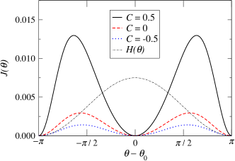
Figure 5: Fisher information $J(\theta)$ obtained for the uncoupled case ($C=0$) and for the coupled cases ($C=\pm 0.5$). Cosine curve in the lower part is the external input (“tuning curve”) $H(\theta)$ given to the system (rescaled and shifted).

5 Stationary information coding efficiency

We first consider the information coding efficiency in the stationary state of our system. In the absence of noise ($D=0$), we can analytically calculate the Fisher information $J(\theta)$ from the self-consistent stationary PDF $P_{0}(\varphi;\theta)$, Eq. (8), as

$$J(\theta)=\frac{1}{2}\left[\frac{\partial F(\theta)}{\partial\theta}\right]^{2}\frac{1}{\left[F(\theta)^{2}-1\right]^{2}}.$$ (13)

Since $F(\theta)$ contains the self-consistent internal field $G_{0}(\theta)$, $J(\theta)$ depends on the mutual coupling through this quantity. By substituting the explicit form of $F(\theta)$, Eq. (11), we can express $J(\theta)$ in terms of $A(\theta)=A+H(\theta)$ and $C\cos\alpha$. When $D>0$, we can calculate $J(\theta)$ using numerically obtained stationary PDFs. With the weak noise we use in this paper, the numerically obtained Fisher information for $D>0$ is close to the noiseless theoretical values at $D=0$.

Figure 5 displays the Fisher information $J(\theta)$ obtained for the uncoupled case ($C=0$) and for the coupled cases ($C=\pm 0.5$) as a function of the external parameter $\theta$. The other parameters are fixed at $A=1.5$, $\alpha=\pi/4$, $H_{0}=0.1$, and $D=0.1$. The Fisher information clearly depends on the coupling strength $C$; we attain much larger value at $C=0.5$ than at $C=0$ or $C=-0.5$. At this noise level, the numerically obtained Fisher information is close to the noiseless theoretical values. Note here that the asynchronous stationary state is unstable without the noise when $C>0$, so that the corresponding theoretical values of the Fisher information cannot be attained in practice. However, as can be seen from Fig. 4, the weak noise ($D=0.1$) can readily stabilize the originally unstable PDF at $C>0$ and helps realize much larger information coding efficiency.

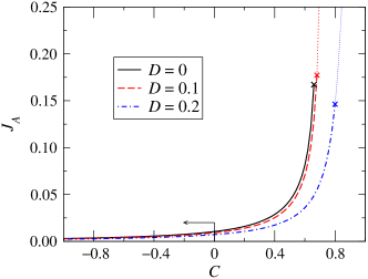
Figure 6: Dependence of the mean Fisher information $J_{A}$ on the coupling strength $C$. At $D=0$, only the region indicated by the arrow can be realized. Crosses represent the values of $C$ where the asynchronous stationary state disappears ($D=0$) or gives way to the stationary fixed state ($D=0.1$, $D=0.2$).

Since our external input $H(\theta)$ takes its maximum value at $\theta=\theta_{0}$, the mean rotation rate of each oscillator is also maximized at this value. However, $J(\theta)$ vanishes at this point, because $\theta=\theta_{0}$ is the extremum of $A(\theta)$, hence $\partial F/\partial\theta\propto\partial A/\partial\theta=0$ holds. Thus, accurate parameter estimation is difficult around $\theta=\theta_{0}$. Rather, $J(\theta)$ takes its maximum at $\theta\simeq\pm\pi/2$, where the functional shape of the stationary PDF most strongly depends on the external parameter $\theta$. This fact is consistent with the results in the previous studies [17, 18, 19], which is interesting since it is against our rate-coding intuition.

In Fig. 6, the dependence of the mean Fisher information $J_{A}=(2\pi)^{-1}\int_{-\pi}^{\pi}J(\theta)d\theta$ on the coupling strength $C$ is displayed at three values of the noise intensity, $D=0$, $D=0.1$, and $D=0.2$. When $D=0$, only the region $C<0$ as indicated in the figure is realizable. However, when $D=0.1$ or $0.2$, originally unstable PDF for $C>0$ is stabilized as shown in Fig. 4, so that the whole curve can be realized. $J_{A}$ increases remarkably as $C$ is increased, because the non-uniformity of the stationary PDF is enhanced, and its dependence on the parameter $\theta$ becomes stronger.

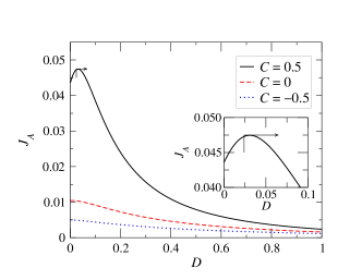
Figure 7: Dependence of the mean Fisher information $J_{A}$ on the noise intensity $D$. At $D=0$, only the region indicated by the arrow can be realized.

If $C$ is further increased to a certain critical value, the stationary PDF corresponding to the asynchronous stationary state disappears ($D=0$) or gives way to the fixed state with low probability flux ($D=0.1$, $D=0.2$). These values are indicated by crosses in the figure. The Fisher information diverges at this point when $D=0$, because the stationary PDF changes its functional form discontinuously. When $D=0.1$ and $D=0.2$, divergence of the Fisher information is suppressed, but it still exhibits abrupt increase due to the sudden change in the stationary PDF. Although this result is formally valid, such divergent behavior indicates the failure of our present framework based on the Fisher information in quantifying the information coding efficiency around bifurcation points; it implies that we can estimate the external parameter with infinite precision even from a single observation. This is due to the basic assumption of our framework, namely, continuous dependence of the functional shape of the PDF on the external parameter, which is generally violated at the bifurcation points. Thus, at present, we consider the divergent behavior of the Fisher information around the bifurcation point as rather a mathematical artifact. In conventional studies of the information coding efficiency using stochastic neuron models [17, 18, 19], the firing statistics of the neurons is usually assumed to be given by some specific family of the PDF, e.g. Gaussian or Poissonian, so that such a situation does not arise generally.

Figure 7 displays the dependence of the mean Fisher information $J_{A}$ on the noise intensity $D$ at three values of the coupling strength, $C=-0.5$, $C=0$, and $C=0.5$. The other parameters are fixed at $A=1.5$, $\alpha=\pi/4$, and $H_{0}=0.1$. As previous, the asynchronous stationary state is unstable at small $D$ when $C=0.5$, and only the region indicated by the arrow in the figure can be realized. As we increase $D$, $J_{A}$ decreases. The noise generally decreases the information coding efficiency of the system, because the noise tends to flatten the stationary PDF and weakens its dependence on $\theta$. However, interestingly, the mean Fisher information $J_{A}$ corresponding to $C=0.5$ takes its maximum value not at $D=0$ but at a small but finite value of $D$, as shown in the inset of Fig. 7 (the asynchronous stationary state is already stabilized at this value of $D$). Thus, the noise is generally disturbing, but it can also help the realization of larger information coding efficiency.

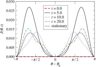
Figure 8: Snapshots of Fisher information $J(\theta,t)$ at several moments in the relaxation process after the onset of the external input.

6 Dynamic information coding efficiency

Since our system is a stochastic dynamical system, we can consider not only its stationary state, but also its non-stationary state. We here briefly study the relaxation process after the presentation of an external input. Let us assume that the system is in its initial asynchronous stationary state without any external input when $t<0$. After $t=0$, we apply a constant external input $H(\theta)$ to the system and observe its relaxation to a new asynchronous stationary state determined by the given parameter $\theta$. By solving the evolution equation (2) of the PDF $P(\varphi,t;\theta)$ numerically, we can calculate the Fisher information $J(\theta,t)$ at any moment.

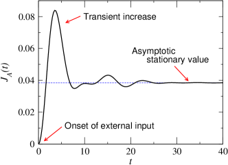
Figure 9: Temporal variation of mean Fisher information $J_{A}(t)$ after the onset of the external input.

Figure 8 shows several snapshots of $J(\theta,t)$ during the relaxation process, and Figure 9 shows temporal variation of the mean Fisher information $J_{A}(t)=(2\pi)^{-1}\int_{-\pi}^{+\pi}J(\theta,t)d\theta$. The system parameters are $A=1.5$, $\alpha=\pi/4$, $C=0.5$, $H_{0}=0.1$, and $D=0.1$. Interestingly, slightly after the onset of the external input, $J(\theta,t)$ exhibits wavy functional shape that is considerably different from the previously obtained stationary functional shape, and then it gradually converges to the stationary shape. Correspondingly, after the onset of the external input, $J_{A}(t)$ rapidly increases from zero to a certain maximum value and then exhibits an oscillatory relaxation to the new stationary value.

This reflects the fact that the dependence of the transient PDF $P(\varphi,t;\theta)$ on $\theta$ is much stronger than that of the stationary PDF $P_{0}(\varphi;\theta)$, which can be qualitatively understood as follows. When we apply a constant external input $H(\theta)$, the PDF undergoes oscillatory relaxation to the new stationary state, with the period of the oscillation determined by the parameter $\theta$. In this process, the discrepancy of two PDFs corresponding to two slightly different values of $\theta$ becomes much larger than that in the stationary state, through a mechanism essentially similar to the “beat” of sound waves. As a result, the Fisher information, which measures the mean response of the PDF to a slight change in the parameter, also increases remarkably and exhibits a transient increase in information coding efficiency.

7 Summary

We considered population coding of an external parameter in the asynchronous state of globally coupled phase oscillators and quantified its information coding efficiency using Fisher information. The Fisher information depends on the mutual coupling through the self-consistent internal field of the oscillators. The noise generally reduces the Fisher information of the system, but it also stabilizes the originally unstable PDF and helps realize larger information coding efficiency. We found a substantial transient increase in Fisher information slightly after the onset of an external input, before the system relaxes to a new stationary state.

Although we treated the information coding only in the asynchronous state in this paper, the fixed or limit-cycle state with sufficiently strong noise may also be considered as the basis for the information coding. It would then be interesting to compare the information coding efficiency among those dynamically distinct situations. However, as we saw in Fig. 6, our framework based on Fisher information does not yield practically meaningful result around the bifurcation point between different dynamical states. To remedy this situation, further modifications to our present framework will be necessary.

The transient increase in Fisher information indicates that the extraction of the information stored in our system can be better achieved in the transient state than in the final stationary state. Though our present system is only a rough caricature of real cortical networks, the mechanism leading such behavior can be generic. Thus, it could provide an interesting viewpoint on the role played by the transient dynamical behavior of the population of real cortical neurons, e.g. in interpreting the results of psychophysical experiments.

In any case, to assert the relevance of our physical findings in the actual information processing by the cortical neurons, we need careful discussions on the physiological plausibility of the model. A more detailed analysis of the present system and generalization to more realistic neural models will be reported in the future.

Finally, from a general viewpoint, our analysis reported in this paper can be considered as a prototypical study of physical systems coding external information. Such a framework would be important in analyzing physical systems that process external information, not only in the context of neuroscience but also in various other areas.

- [1] C. M. Gray and W. Singer, Proc. Natl. Acad. Sci. USA 86, 1698 (1989).
- [2] A. K. Engel, A. K. Kreiter, P. König, and W. Singer, Proc. Natl. Acad. Sci. USA 88, 6048 (1991).
- [3] F. Varela, J.-P. Lachaux, E. Rodriguez, and J. Martinerie, Nature Rev. Neurosci. 2, 229 (2001).
- [4] E. Salinas and T. J. Sejnowski, Nature Rev. Neurosci. 2, 539 (2001).
- [5] D. Golomb, D. Hansel, B. Shraiman, and H. Sompolinsky, Phys. Rev. A 45, 3516 (1992).
- [6] G. B. Ermentrout and D. Kleinfeld, Neuron 29, 33 (2001).
- [7] Y. Kuramoto, Chemical Oscillations, Waves, and Turbulence (Springer-Verlag, Berlin, 1984).
- [8] Y. Kuramoto, Physica D 50 (1991) 15.
- [9] A. Pikovsky, M. Rosenblum, and J. Kurths, Synchronization (Cambridge University Press, Cambridge, 2001).
- [10] W. R. Softky and C. Koch, Neural Comput. 4, 643 (1992).
- [11] L. F. Abbott and C. van Vreeswijk, Phys. Rev. E 48, 1483 (1993).
- [12] W. Gerstner, Neural Comput. 12, 43 (2000).
- [13] D. Hansel and G. Mato, Phys. Rev. Lett. 86, 4175 (2001).
- [14] D. J. Mar, C. C. Chow, W. Gerstner, R. W. Adams, and J. J. Collins, Proc. Natl. Acad. Sci. USA 96, 10450 (1999).
- [15] D. Q. Nykamp and D. Tranchina, Journal of Computational Neuroscience 8, 19 (2000).
- [16] A. Omurtag, E. Kaplan, B. Knight, and L. Sirovich, Network: Comput. Neural Syst. 11, 247 (2000).
- [17] M. A. Paradiso, Biol. Cybern. 58, 35 (1988).
- [18] H. S. Seung and H. Sompolinsky, Proc. Natl. Acad. Sci. USA 90, 10749 (1993).
- [19] L. Abbott and T. J. Sejnowski, eds., Neural Codes and Distributed Representations: Foundations of Neural Computation (MIT Press, Cambridge, 1999).
- [20] E. L. Lehman, Theory of Point Estimation (Wiley, New York, 1983).
- [21] T. M. Cover and J. A. Thomas, Elements of Information Theory (Wiley, New York, 1991).