Exact hydrodynamics of a trapped dipolar Bose-Einstein condensate

The current revolution in the cooling of atomic gases to ultra-cold temperatures has led to the experimental realization of a number of highly idealized and fundamental regimes in the quantum physics of many-particle systems [1, 2]. For example, in a Bose-Einstein condensed gas containing several million atoms the zero-point kinetic energy can be negligible in comparison to the interparticle interaction energy. In this so-called Thomas-Fermi regime the collective dynamics of the Bose-Einstein condensate (BEC) are described by the collisionless hydrodynamic theory of Bose superfluids at zero temperature [3]. Furthermore, the interparticle interactions can be directly manipulated using external electromagnetic fields, giving a degree of freedom not normally available in the systems traditionally studied in statistical physics. The dominant interactions in these gases are usually of the van der Waals type, decaying as $r^{-6}$, short-ranged in comparison to the interatomic separation. This permits an effective description of the interactions solely in terms of the $s$-wave scattering length, $a_{\mathrm{s}}$. Within the mean-field scheme of the Gross-Pitaevskii equation [4] the interactions are modelled by the contact pseudo-potential, $g\delta({\bf r})\equiv(4\pi a_{\mathrm{s}}\hbar^{2}/m)\delta({\bf r})$, where $m$ is the atomic mass, and $g$ incorporates the quantum aspects of low-energy scattering. By using a magnetic field to induce a Feshbach resonance during atomic collisions, one can adjust the value of $a_{\mathrm{s}}$ between positive (repulsive) and negative (attractive) values [5].

Here we consider a harmonically trapped BEC which, as well as van der Waals interactions, also has dipole-dipole interactions. Such a system was first considered by Yi and You [6] in the context of dipoles induced by an external electric field and by Góral, Rza̧żewski, and Pfau [7] in the context of permanent magnetic dipoles aligned by an external magnetic field. In comparison to van der Waals interactions, dipole-dipole interactions have a much longer range and are anisotropic. This has been predicted to lead to BECs with unusual stability properties [8, 9], exotic ground states such as supersolid [10, 11] and checkerboard phases [11], and modified excitation spectra [12, 13] even to the extent of a roton minimum [14]. Dipole-dipole interactions are also inherently controllable, either via the magnitude of the external electric field in the case of electrically induced dipoles, or in the case of permanent dipoles by modulating the external aligning field in time [15], which allows control over both the magnitude and sign of the dipolar interactions.

The long-range part of the interaction between two dipoles separated by ${\bf r}$, and aligned by an external field along a unit vector $\hat{\mathbf{e}}$, is given by

$$U_{\mathrm{dd}}({\bf r})=\frac{C_{\mathrm{dd}}}{4\pi}\,\hat{{\rm e}}_{i}\hat{{\rm e}}_{j}\frac{\left(\delta_{ij}-3\hat{r}_{i}\hat{r}_{j}\right)}{r^{3}}$$ (1)

where the coupling $C_{\mathrm{dd}}/(4\pi)$ depends on the specific realization. Electric dipoles induced by an external static electric field $\mathbf{E}=E\hat{\mathbf{e}}$ have $C_{\mathrm{dd}}=E^{2}\alpha^{2}/\epsilon_{0}$ [6], where $\alpha$ is the static polarizability. For magnetic atoms with magnetic dipole moment $d_{m}$ aligned by an external magnetic field $\mathbf{B}=B\hat{\mathbf{e}}$, then $C_{\mathrm{dd}}=\mu_{0}d_{m}^{2}$. A measure of the strength of the dipole-dipole interaction relative to the short-range van der Waals $s$-wave scattering energy is given by the dimensionless quantity

$$\varepsilon_{\mathrm{dd}}\equiv\frac{C_{\mathrm{dd}}}{3g}\ .$$ (2)

For $\varepsilon_{\mathrm{dd}}>1$ instabilities are expected [7, 15] in the limit of negligible kinetic energy. Note that the value of $g$ can be altered in the presence of a strong external electric field [12]. Alkali atoms can have a magnetic dipole moment of $d_{m}=1\mu_{\mathrm{B}}$ (Bohr magneton), and for ⁸⁷Rb, which has $a_{\mathrm{s}}\approx 103\mathrm{a}_{0}$ (Bohr radius), one finds $\varepsilon_{\mathrm{dd}}\approx 0.007$. Na has $\varepsilon_{\mathrm{dd}}\approx 0.004$, and accordingly magnetic dipolar effects in BECs of these atoms are expected to be small, at least in a stationary condition. The effects of the dipolar interactions can be made visible by rotating the magnetic field in resonance with a collective excitation frequency of the system [15]. Also, using a Feshbach resonance to reduce $a_{\mathrm{s}}$ could substantially increase $\varepsilon_{\mathrm{dd}}$ [16]. However, a good candidate atom for a dipolar BEC is chromium which has $d_{m}=6\mu_{\mathrm{B}}$. The $s$-wave scattering length of ⁵²Cr, the more common isotope, is $170\pm 40$ a₀. Consequently for that isotope $\varepsilon_{\mathrm{dd}}\approx 0.089$. The less common isotope ⁵⁰Cr has $a_{\mathrm{s}}=40\pm 15$ a₀, and $\varepsilon_{\mathrm{dd}}\approx 0.36$ is much higher. A chromium BEC does not yet exist, but a program of experiments is underway with that goal in mind [17]. Using a crossed optical trap, like in the recent cesium condensation experiment [18], atom numbers in a ⁵²Cr BEC on the order of $N=10^{4}$ might be within reach, and the radial and longitudinal frequencies of the cylindrically symmetric (optical) harmonic confinement would be in the region of $\omega_{x}=\omega_{y}=2\pi 170$ s^-1 and $\omega_{z}=2\pi 240$ s^-1, respectively [17]. The trap anisotropy $\gamma=\omega_{z}/\omega_{x}=1.41$ is optimal for enhancing the condensate shape deformations [19]. For a harmonically trapped BEC with just $s$-wave scattering the Thomas-Fermi limit is reached for large values of the dimensionless parameter $Na_{\mathrm{s}}/a_{\mathrm{ho}}$ [2] where $a_{\mathrm{ho}}=\sqrt{\hbar/m\omega}$ is the harmonic oscillator length of the trap, and $N$ is the total number of atoms. For ⁵²Cr one has $Na_{\mathrm{s}}/a_{\mathrm{ho}}\approx 90$, illustrating that the Thomas-Fermi regime is an appropriate starting point for analyzing these experiments.

The application of collisionless hydrodynamics to an ordinary BEC is based upon the existence of a macroscopic condensate order parameter $\psi({\bf r},t)=\sqrt{n({\bf r},t)}\exp\mathrm{i}\phi({\bf r},t)$, normalized to $N$, consisting of density $n({\bf r},t)$, and phase $\phi({\bf r},t)$. The phase determines the superfluid velocity via potential flow, $\mathbf{v}({\bf r},t)=(\hbar/m)\mathbf{\nabla}\phi({\bf r},t)$. The nonlinear evolution of the condensate in the Thomas-Fermi regime is then dictated by the continuity and Euler equations given by, respectively,

$${\partial n\over\partial t} = -{\bf\nabla}\cdot(n{\bf v})\;,$$ (3)

$$m{\partial{\bf v}\over\partial t} = -{\bf\nabla}\left(\frac{mv^{2}}{2}+V_{\mathrm{ext}}+gn\right)\;.$$ (4)

$V_{\mathrm{ext}}$ is the external potential, which is provided by the harmonic trap, $V_{\mathrm{ext}}({\bf r})=m(\omega_{x}^{2}x^{2}+\omega_{y}^{2}y^{2}+\omega_{z}^{2}z^{2})/2$. Eqs.  (3) and (4) describe the potential flow of a fluid whose pressure and density are related by the equation of state $P=(g/2)n^{2}$, and are equivalent to the time dependent Gross-Pitaevskii equation [4] when the zero-point fluctuation term $(-\hbar^{2}\nabla^{2}\sqrt{n}/2m\sqrt{n})$ is included in the brackets on the right hand side of (4) after the Bernoulli term $mv^{2}/2$. The equilibrium solution of (3) and (4), which has ${\bf v}=0$, is the well known Thomas-Fermi inverted parabola density profile

$$n({\bf r})=[\mu-V_{\mathrm{ext}}({\bf r})]/g\ \ \mbox{ for }\ n({\bf r})\geq 0,$$ (5)

and $n({\bf r})=0$ elsewhere. Thus the density profile is completely determined by the trapping potential, having the same aspect ratio as the trap.

An analysis of the dynamical (${\bf v}\neq 0$) solutions of (3) and (4) has been given by Stringari [3]. However, motivated by the experimental possibility of changing the trapping frequencies in time, so that $\omega_{j}\rightarrow\omega_{j}(t)$ with $j=x,y,z$, Kagan, Surkov, and Shlyapnikov [20] and Castin and Dum [21] studied a special class of “scaling” solution, valid for time-dependent harmonic traps, corresponding to [2]

$$n({\bf r},t) = n_{0}(t)\left[1-\frac{x^{2}}{R_{x}^{2}(t)}-\frac{y^{2}}{R_{y}^{2}(t)}-\frac{z^{2}}{R_{z}^{2}(t)}\right]\;,$$ (6)

$${\bf v}({\bf r},t) = \frac{1}{2}\mathbf{\nabla}\left[\alpha_{x}(t)x^{2}+\alpha_{y}(t)y^{2}+\alpha_{z}(t)z^{2}\right]$$ (7)

valid where $n({\bf r},t)\geq 0$ and $n({\bf r},t)=0$ elsewhere. The central density $n_{0}(t)$ is constrained by normalization to be $n_{0}(t)=15N/[8\pi R_{x}(t)R_{y}(t)R_{z}(t)]$. The time-evolution of the radii $R_{j}$ reduces to the solution of three ordinary differential equations, and the components of the velocity field, $\alpha_{j}$, depend on the corresponding radii as $\alpha_{j}=\dot{R}_{j}/R_{j}$. Although these scaling solutions represent only a limited class of the possible solutions to the hydrodynamic equations, they model two crucial experimental situations: i) the expansion of a BEC when the trap is relaxed or turned off—this is usually necessary to image the BEC which would otherwise be too small in situ (time of flight measurements then record the original momentum distribution); ii) the response of the BEC to a modulation of the trapping frequencies, which is the easiest way to generate shape oscillations of the BEC.

The existence of the class (6) of analytic scaling solutions relies upon a harmonic trap and the local character of $s$-wave interactions. The remainder of this paper demonstrates an analogous exact result for a dipolar BEC. This result is not obvious because of the non-local nature of dipolar interactions. Nevertheless, it turns out that the dipolar contribution to the mean-field potential generated by a parabolic density profile is itself also parabolic so that (6) and (7) still represent a self-consistent solution to the hydrodynamic equations of motion.

Exact static solution for a Thomas-Fermi dipolar BEC — Dipolar interactions can be included in a mean-field treatment of the BEC via a Hartree potential

$$\Phi_{\mathrm{dd}}({\bf r})\equiv\int{\rm d}^{3}r^{\prime}\ U_{\mathrm{dd}}({\bf r}-{\bf r}^{\prime})n({\bf r}^{\prime})$$ (8)

as shown by Yi and You [12] based on a calculation of the two-body T-matrix. The hydrodynamic equations of motion for dipolar BEC are then the same as above but with the Euler equation (4) supplemented by adding $\Phi_{\mathrm{dd}}({\bf r})$ into the bracket on the r.h.s. We begin our analysis with a suggestive re-casting of the dipole-dipole term (1)

$$\frac{\left(\delta_{ij}-3\hat{r}_{i}\hat{r}_{j}\right)}{4\pi r^{3}}=-\nabla_{i}\nabla_{j}\frac{1}{4\pi r}-\frac{1}{3}\delta_{ij}\delta({\bf r})\;.$$ (9)

We can then write

$$\Phi_{\mathrm{dd}}({\bf r}) =-C_{\mathrm{dd}}\>\left(\hat{\mathrm{e}}_{i}\hat{\mathrm{e}}_{j}\nabla_{i}\nabla_{j}\phi({\bf r})+\frac{1}{3}n({\bf r})\right)$$ (10)

$$\mbox{with }\ \phi({\bf r}) \equiv\frac{1}{4\pi}\int\frac{{\rm d}^{3}r^{\prime}\;n({\bf r}^{\prime})}{|{\bf r}-{\bf r}^{\prime}|}\;.$$ (11)

The problem thereby reduces to an analogy with electrostatics, and one need only calculate the ‘potential’ $\phi({\bf r})$ arising from the ‘static charge’ distribution $n({\bf r})$. We are now in a position to see the basic form $n({\bf r})$ must take, since $\phi({\bf r})$ given by (11) obeys Poisson’s equation $\nabla^{2}\phi=-n({\bf r})$. Thus, if the density is parabolic, of the form (6), then Poisson’s equation is satisfied by a potential of the form $\phi=a_{0}+a_{1}x^{2}+a_{2}y^{2}+a_{3}z^{2}+a_{4}x^{2}y^{2}+a_{5}x^{2}z^{2}+a_{6}y^{2}z^{2}+a_{7}x^{4}+a_{8}y^{4}+a_{9}z^{4}$, and by (10) $\Phi_{\mathrm{dd}}({\bf r})$ is also parabolic. Therefore, an inverted parabola remains a self-consistent solution to the dipolar hydrodynamic equations. The evaluation of the integral (11) is too long to be reproduced here [22], but can be achieved either by integrating over successive thin ellipsoidal shells, or in the case of cylindrical symmetry by transforming into spheroidal coordinates and using the known Green’s function for Poisson’s equation in that basis.

For simplicity (though not necessity), we shall restrict attention to cylindrical symmetry for both trap and BEC about the $z$ axis, along which the external polarizing field is understood to point. Thus we have $R_{x}=R_{y}$ for the BEC and $V_{\mathrm{ext}}=(m/2)[\omega_{x}^{2}\rho^{2}+\omega_{z}^{2}z^{2}]$, where $\rho^{2}=x^{2}+y^{2}$, for the trap. Then, inside the condensate region, the dipolar potential (10) generated by an inverted parabola density distribution (6) of dipoles, is [22]

$$\Phi_{\mathrm{dd}}=\frac{n_{0}C_{\mathrm{dd}}}{3}\left[{\rho^{2}\over R_{x}^{2}}-{2z^{2}\over R_{z}^{2}}-f\left(\kappa\right)\left(1-\frac{3}{2}{\rho^{2}-2z^{2}\over R_{x}^{2}-R_{z}^{2}}\right)\right]$$ (12)

$$\mbox{where}\quad f(\kappa)=\frac{1+2\kappa^{2}}{1-\kappa^{2}}-\frac{3\kappa^{2}\mathrm{arctanh}\sqrt{1-\kappa^{2}}}{\left(1-\kappa^{2}\right)^{3/2}}\quad$$ (13)

with $\kappa\equiv R_{x}/R_{z}$ being the condensate aspect ratio. We recover the result (9) of [15] in the particular case of a spherical dipolar condensate ($R_{x}=R_{z}$). In order to determine the equilibrium values of $R_{x}$ and $R_{z}$, the result (12) for $\Phi_{\mathrm{dd}}$ should be substituted into the Euler equation (4) with ${\bf v}=0$, giving a transcendental equation for the aspect ratio $\kappa$ [12]

$$3\kappa^{2}\varepsilon_{\mathrm{dd}}\left[\left(\frac{\gamma^{2}}{2}+1\right)\frac{f(\kappa)}{1-\kappa^{2}}-1\right]+\left(\varepsilon_{\mathrm{dd}}-1\right)\left(\kappa^{2}-\gamma^{2}\right)=0$$ (14)

where $\gamma=\omega_{z}/\omega_{x}$ is the ratio of the harmonic trapping frequencies. Fig. 1 shows some examples of the dependence of $\kappa$ upon $\varepsilon_{\mathrm{dd}}$ for oblate, spherical and prolate traps.

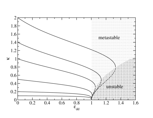
Figure 1: Equilibrium aspect ratio $\kappa$ of the BEC, as a function of the dipole-dipole to $s$-wave coupling ratio, $\varepsilon_{\mathrm{dd}}$. Each line is for a trap of a different aspect ratio $\gamma$ ($\kappa=\gamma$ when $\varepsilon_{\mathrm{dd}}=0$). When $0<\gamma\ [\kappa]<1$ the trap $[\mbox{condensate}]$ is prolate, $\gamma\ [\kappa]>1$ the trap $[\mbox{condensate}]$ is oblate. The dashed lines indicate an unstable branch. However, local density perturbations most likely render the condensate unstable whenever $\varepsilon_{\mathrm{dd}}>1$.

The effect of the dipole-dipole forces polarized along the $z$-axis is to make the condensate more cigar-shaped along $z$. For an oblate trap ($\gamma>1$) the BEC becomes exactly spherical when $\varepsilon_{\mathrm{dd}}=(5/2)(\gamma^{2}-1)/(\gamma^{2}+2)$. An analysis of the energy functional associated with the scaling solution (6) shows that when $\varepsilon_{\mathrm{dd}}>1$ the solution loses its global stability to scaling perturbations and is only metastable [8, 12, 22] (only a local minimum of the energy), the global minimum being a collapsed pencil-like prolate state. Increasing $\varepsilon_{\mathrm{dd}}$ yet further, the scaling solution ceases to exist entirely in the region marked as unstable in Fig. 1. However, we strongly caution the reader that any state of a dipolar BEC with $\varepsilon_{\mathrm{dd}}>1$ is probably unattainable since other classes of perturbations (that do not respect the scaling form (6)), such as local phonons, render the dipolar BEC unstable to collapse whenever $\varepsilon_{\mathrm{dd}}>1$ [7, 15].

A moment’s thought shows that the aspect ratio is independent of the specifics of the density profile and indeed the same transcendental Eq. (14) has been previously obtained using a Gaussian ansatz [12]. However, what is specific to the exact solution are the absolute radii which, once (14) has been solved for $\kappa$, are given by

$$\displaystyle R_{x}=R_{y}=\left[\frac{15gN\kappa}{4\pi m\omega_{x}^{2}}\left\{1+\displaystyle\varepsilon_{\mathrm{dd}}\left(\frac{3}{2}\frac{\kappa^{2}f(\kappa)}{1-\kappa^{2}}-1\right)\right\}\right]^{1/5}$$ (15)

and $R_{z}=R_{x}/\kappa$. If the trap is turned off the $s$-wave and dipole-dipole interaction energies are converted into kinetic energy, the so-called release energy $E_{\mathrm{rel}}$, which can be directly measured in an experiment. One finds $E_{\mathrm{rel}}=15gN^{2}[1-\varepsilon_{\mathrm{dd}}f(\kappa)]/(28\pi R_{x}^{2}R_{z})$.

Exact scaling hydrodynamics of a dipolar condensate — The parabolic form of $\Phi_{\mathrm{dd}}({\bf r})$ means that the scaling solutions [20, 21] for dynamics also apply to a dipolar BEC. Substituting the scaling solutions (6) and (7) into the continuity and Euler equations yields the following classical equations of motion for the radii

$$\ddot{R}_{x} = -\omega_{x}^{2}(t)R_{x}+\frac{15gN}{4\pi mR_{x}R_{z}}\bigg{[}\frac{1}{R_{x}^{2}}$$ (16)

$$\mbox{ \hskip 10.00002pt}-\varepsilon_{\mathrm{dd}}(t)\left(\frac{1}{R_{x}^{2}}+\frac{3}{2}\frac{f(R_{x}/R_{z})}{R_{x}^{2}-R_{z}^{2}}\right)\bigg{]}$$

$$\ddot{R}_{z} = -\omega_{z}^{2}(t)R_{z}+\frac{15gN}{4\pi mR_{x}^{2}}\bigg{[}\frac{1}{R_{z}^{2}}$$ (17)

$$\mbox{ \hskip 10.00002pt}+2\varepsilon_{\mathrm{dd}}(t)\left(\frac{1}{R_{z}^{2}}+\frac{3}{2}\frac{f(R_{x}/R_{z})}{R_{x}^{2}-R_{z}^{2}}\right)\bigg{]}.$$

Solving these equations under particular choices of the dependence of $\omega_{j}(t)$ upon time gives the evolution of the density and phase of the condensate when undergoing e.g. free expansion (trap switched off), or shape oscillations (time-modulation of the trap). A time-dependent dipolar coupling is also possible as explicitly indicated. As mentioned above, our results show that previous calculations based upon the Gaussian variational ansatz of the aspect ratio $\kappa(t)$ during ballistic expansion [19], or during the parametric excitation of the quadrupole shape oscillation mode using dipolar interactions as a time-dependent coupling [15], are exact in the Thomas-Fermi limit.

Linearizing (16–17) around the equilibrium solution (15) gives the following frequencies for small amplitude scaling oscillations

$$\Omega_{\pm}^{2}=\frac{1}{2}\left(h_{xx}+h_{zz}\pm\sqrt{(h_{xx}-h_{zz})^{2}+4h_{xz}h_{zx}}\right)$$ (18)

where

$$h_{xx} = \omega_{x}^{2}+3\omega_{x}^{2}\frac{1-\varepsilon_{\mathrm{dd}}\left[\frac{1-2\kappa^{2}}{1-\kappa^{2}}+\frac{\kappa^{2}(4\kappa^{2}+1)f(\kappa)}{2(1-\kappa^{2})^{2}}\right]}{1+\varepsilon_{\mathrm{dd}}\left[\frac{3\kappa^{2}f(\kappa)}{2(1-\kappa^{2})}-1\right]}$$

$$h_{zz} = \gamma^{2}\omega_{x}^{2}+2\omega_{x}^{2}\kappa^{2}\frac{1+\varepsilon_{\mathrm{dd}}\left[\frac{5-2\kappa^{2}}{1-\kappa^{2}}-\frac{3(\kappa^{2}+4)f(\kappa)}{2(1-\kappa^{2})^{2}}\right]}{1+\varepsilon_{\mathrm{dd}}\left[\frac{3\kappa^{2}f(\kappa)}{2(1-\kappa^{2})}-1\right]}$$

$$h_{zx} = 2h_{xz}=2\omega_{x}^{2}\kappa\frac{1-\varepsilon_{\mathrm{dd}}\left[\frac{1+2\kappa^{2}}{1-\kappa^{2}}-\frac{15\kappa^{2}f(\kappa)}{2(1-\kappa^{2})^{2}}\right]}{1+\varepsilon_{\mathrm{dd}}\left[\frac{3\kappa^{2}f(\kappa)}{2(1-\kappa^{2})}-1\right]}\ .$$ (19)

$\Omega_{-}$ corresponds to quadrupole, and $\Omega_{+}$ to monopole (breathing) shape oscillations, respectively [12, 13], see Fig. 2. Note that the frequencies do not depend on $g$ directly, only through $\varepsilon_{\mathrm{dd}}$. Fig. 3 illustrates that certain trap anisotropies maximise the effects of the dipolar interactions upon the collective excitation frequencies.

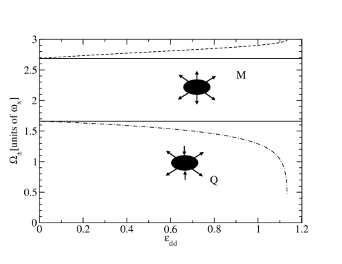
Figure 2: The monopole (dashed) and quadrupole (dash-dotted) oscillation frequencies in units of the radial trapping frequency, as functions of $\varepsilon_{\mathrm{dd}}$. The solid lines are for a BEC with only $s$-wave contact interactions, $\Omega_{\pm}^{0}$. The trap aspect ratio is set at $\gamma=240/170$. The frequencies become complex at precisely the value of $\varepsilon_{\mathrm{dd}}$ at which the equilibrium solution becomes unstable. However, other instabilities, due to phonons, are possible whenever $\varepsilon_{\mathrm{dd}}>1$.

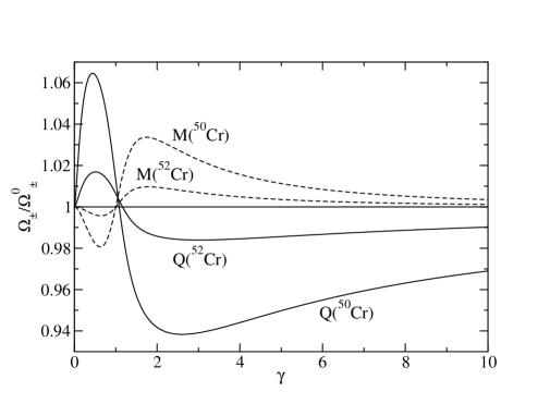
Figure 3: The monopolar (dashed) and quadrupolar (solid) frequencies as fractions of their $s$-wave-only frequencies, $\Omega_{\pm}^{0}$, of ⁵²Cr ($\varepsilon_{\mathrm{dd}}=0.089$) and ⁵⁰Cr ($\varepsilon_{\mathrm{dd}}=0.36$), plotted as functions of the trap anisotropy $\gamma$.

Conclusion — Dipolar condensates promise to open a new chapter in the study of controllable superfluids. At first sight, the non-local and anisotropic form of dipolar interactions also make the elucidation of the static and excited states of a dipolar BEC non-trivial, i.e. direct numerical calculation is for instance computationally heavy in comparison to standard BECs with contact interactions. We have shown, however, that there exist simple exact solutions which should prove useful for quantitative analysis of upcoming experiments.

It is a pleasure to thank Gabriel Barton for discussions and Tilman Pfau and his group for sharing their results with us. We would like to acknowledge financial support from the UK Engineering and Physical Sciences Research Council (D.O’D.), the European Union (S.G.), and the Royal Society (C.E.).

- [1] W. Ketterle, D.S. Durfee and D.M. Stamper-Kurn, Proc. Int. Sch. Phys. “Enrico Fermi”, Course CXL, edited by M. Inguscio, S. Stringari and C.E. Wieman (IOS Press, Amsterdam, 1999).
- [2] F. Dalfovo, S. Giorgini, L.P. Pitaevskii and S. Stringari, Rev. Mod. Phys. 71, 463 (1999).
- [3] S. Stringari, Phys. Rev. Lett. 77, 2360 (1996).
- [4] L.P. Pitaevskii, Sov. Phys. JETP, 13, 451 (1961); E.P. Gross, Nuovo Cimento 20, 454 (1961); J. Math. Phys. 4, 195 (1963).
- [5] S. Inouye, M.R. Andrews, J. Stenger, H.-J. Miesner, D.M. Stamper-Kurn, and W. Ketterle, Nature 392, 151 (1998).
- [6] S. Yi and L. You, Phys. Rev. A 61, 041604 (2000).
- [7] K. Góral, K. Rza̧żewski, and T. Pfau, Phys. Rev. A 61, 051601 (2000); J.-P. Martikainen, M. Mackie, and K.-A. Suominen, Phys. Rev. A 64, 037601 (2001).
- [8] L. Santos, G.V. Shlyapnikov, P. Zoller, and M. Lewenstein, Phys. Rev. Lett. 85, 1791 (2000).
- [9] P.M. Lushnikov, Phys. Rev. A 66, 051601(R) (2002).
- [10] S. Giovanazzi, D. O’Dell, and G. Kurizki, Phys. Rev. Lett. 88, 130402 (2002).
- [11] K. Góral, L. Santos, and M. Lewenstein, Phys. Rev. Lett. 88, 170406 (2002).
- [12] S. Yi and L. You, Phys. Rev. A 63, 053607 (2001); ibid. 66, 013607 (2002).
- [13] K. Góral and L. Santos, Phys. Rev. A 66, 023613 (2002).
- [14] D.H.J. O’Dell, S. Giovanazzi and G. Kurizki, Phys. Rev. Lett. 90, 110402 (2003); L. Santos, G.V. Shlyapnikov, and M. Lewenstein, Phys. Rev. Lett. 90, 250403 (2003).
- [15] S. Giovanazzi, A. Görlitz and T. Pfau, Phys. Rev. Lett. 89, 130401 (2002).
- [16] S. Yi and L. You, Phys. Rev. A 67, 045601 (2003).
- [17] S. Hensler and T. Pfau, private communication.
- [18] T. Weber, J. Herbig, M. Mark, H-C. Nägerl and R. Grimm, Science, 299, 232 (2003).
- [19] S. Giovanazzi, A. Görlitz and T. Pfau, J. Opt. B 5 S208 (2003).
- [20] Yu. Kagan, E.L. Surkov, and G.V. Shlyapnikov, Phys. Rev. A 54, 1753 (1996); ibid. 55, 18 (1997).
- [21] Y. Castin, and R. Dum, Phys. Rev. Lett. 77, 5315 (1996).
- [22] D.H.J. O’Dell, S. Giovanazzi and C. Eberlein, unpublished.