On the break in the single-particle energy dispersions and
the ‘universal’ nodal Fermi velocity in the
high-temperature copper oxide superconductors
Behnam FaridSpinoza Institute, Department of Physics and Astronomy,
University of Utrecht,
Leuvenlaan 4, 3584 CE Utrecht, The Netherlands
***Electronic address: B.Farid@phys.uu.nl.
Abstract
Recent data from angle-resolved photoemission experiments published
by Zhou et al. [Nature, 423, 398 (2003)] concerning
a number of hole-doped copper-oxide based high-temperature
superconductors reveal that in the nodal directions of the underlying
square Brillouin zones (i.e. the directions along which the
-wave superconducting gap is vanishing) the Fermi velocities
for some finite range of inside the Fermi sea and away from
the nodal Fermi wave vector are to within an
experimental uncertainty of approximately % the same both in
all the compounds investigated and over a wide range of doping
concentrations and that, in line with earlier experimental
observations, at some characteristic wave vector
away from (
typically amounts to approximately % of )
the Fermi velocities undergo a sudden change, with this change (roughly
speaking, an increase for )
being the greatest (smallest) in the case of underdoped (overdoped)
compounds. We demonstrate that these observations establish
four essential facts: firstly, the ground-state momentum
distribution function must be discontinuous at
; with
and denoting the measured velocities
close to , , and ,
we obtain
(1)
in which is the ‘Fermi’ velocity
corresponding to the case in which (for
two-body interaction potentials of shorter range than the Coulomb
potential, whereby
);
secondly, the single-particle spectral function
must at possess a coherent contribution
corresponding to a well-defined quasiparticle excitation at an energy
of approximately meV below the Fermi energy; thirdly, the amount
of discontinuity in at the
nodal Fermi points must be small and ideally vanishing;
fourthly, the long range of the two-body Coulomb potential is of
vital importance for realization of a certain aspect of the
observed behaviour in the Fermi velocities (specifically) in the
underdoped regime. The condition conforms
with the observation through an earlier angle-resolved photoemission
experiment by Valla et al. [Science, 285, 2110
(1999)], on the optimally doped compound
Bi2Sr2CaCu2O8+δ, which shows that the imaginary part
of the self-energy along the nodal directions of the Brillouin zone
and in the vicinity of the nodal Fermi points satisfies the scaling
behaviour characteristic of marginal Fermi-liquid metallic states, for
which is indeed vanishing. We present arguments
advocating the viewpoint that the observed ‘kink’ in the measured
energy dispersions cannot be a direct consequence of
electron-phonon interaction, although a finite
may possibly arise from this interaction. In other words, even though
possibly vital, the role played by phonons in bringing about the latter
‘kink’ must be indirect. Our approach further provides a consistent
interpretation of the observed sudden decrease in the width of the
so-called ‘momentum distribution curve’ on increasing
above .
Angle-resolved photoemission spectroscopy (ARPES) [1, 2]
provides information with regard to the single-particle spectral
function of systems for , where is the external energy parameter,
the chemical potential, the wave vector and
the spin index. The quantity measured experimentally is the
photoelectron intensity which at
finite temperature and under some specified approximations is
proportional to ,
where is the Fermi
distribution function [1, 2]. The experimental results
obtained by Zhou et al.[3] and other workers
[4, 5, 6, 7, 8], to be discussed in the present
paper, are deduced from the so-called ‘momentum distribution curve’
(MDC); this curve is obtained by setting out along the desired directions in the space
for a fixed value of . A related curve, referred to as
the ‘energy distribution curve’ (EDC), is obtained by plotting
for a fixed along the
axis. Amongst others, the determination of the peak
positions in from the corresponding
MDC does not suffer from the ambiguities associated with
.
In this paper we first consider the relationship between the
energy dispersions as measured in angle-resolved photoemission
experiments and the single-particle excitation energy dispersions
as determined by solving the quasi-particle equation in terms
of the self-energy operator; the latter accounts for the correlation
in the ground states (GSs) of the underlying systems. The formalism
concerning the measured energy dispersions that follows from our
purely heuristic arguments turns out to coincide, in all details, with
that developed by the present author in his recent investigations
regarding the nature of the uniform metallic GSs of the conventional
single-band Hubbard Hamiltonian [9] and more general
single-band Hamiltonians [10] in which the particle-particle
interaction can be of arbitrary range. The specific aspects of the
formalism developed in [9, 10] that greatly suited the
aims in the aforementioned investigations are that for the indicated
GSs it formally yields
(i) the exact GS total energy,
(ii) the exact Fermi energy, (iii) the exact Fermi surface and (iv) the exact momentum distribution function.
The formalism has made possible [9, 10] to make exact
predictions concerning the values that the GS momentum distribution
function can take for in the
close neighbourhoods of the underlying Fermi surface
. On the basis of this, it has been
possible to expose [10] the significant influence that
the range of the two-body interaction potential can have on
and consequently on the partitioning
of the GS total energy into ‘kinetic’ and ‘interaction’ parts.
This observation led us to the conclusion [10] that the
experimentally-inferred excess ‘kinetic’ energy in the normal
states of the copper-oxide based high-temperature superconductors
[11, 12] (for other pertinent references see [10])
may be signifying the importance of the long range of the two-body
interaction potential in determining other distinctive aspects of
the normal metallic states of these compounds that mark them as
unconventional metals [13].
For the normal uniform metallic GSs of the single-band Hubbard
Hamiltonian, we have established that, so long as these are Fermi
liquids, for inside the Fermi sea and close to the Fermi
surface, a single-particle energy dispersion , which in [9, 10] was attributed to some
‘fictitious’ particles and in this paper we reason to be the one
measured through the ARPES, is up to a multiplicative
-independent constant equal to the energy dispersion
of the Landau quasi-particles
inside the Fermi sea (more precisely, the energy dispersion
as obtained from the quasi-particle
equation in Eq. (4) below; see § 3.1); similarly for
(Eq. (25)) and
concerning outside the
Fermi sea. For cases where the two-particle interaction potential
is the long-range Coulomb potential, in [10] it was however
shown that no such strict relationship exists between
(and similarly
) and (), not even for Fermi
liquid metallic states. In this paper we rigorously demonstrate
that in spite of these aspects, in cases where for a given the quasi-particle equation (Eq. (4) below)
has solutions and
corresponding to
well-defined Landau quasi-particles, irrespective of the nature of
the two-body interaction potential identically coincides with (if is continuous
at ; Eq. (30)) and
with
(if
is continuous at ; Eq. (33)); we present the appropriate
expressions for and
in terms of
and
respectively for
cases in which either or both of
and are discontinuous at ; according to our analysis (§ 3.4), these
functions cannot both be continuous at .
In the light of the above-mentioned similarities between
and the possible solutions
of the quasi-particle equation
associated with particle-like excitations (as opposed to collective
low-lying excitations in non-Fermi-liquid metallic states) as well
as the heuristic arguments underlying the definition of
(see § 2), in this paper we
assert that the ARPES data concerning the dispersion of the
single-particle excitation energies are to be compared with
. The fact that the behaviour
of corresponding to Fermi-liquid
metallic states of systems of fermions interacting through the
long-range Coulomb potential in the neighbourhood of
demonstrably differs from that of the
asymptotic solution (see § 3.1) of
the quasi-particle equation in the neighbourhood of (see above) does not diminish the strength of our arguments.
In this connection we should emphasize that our assertion has bearing
on the energy dispersions as measured by means of the ARPES and
thus does not negate the fundamental significance of the possible
asymptotic solutions of the quasi-particle equation, nor the essential
role that these (explicitly, the asymptotic solutions corresponding to
the exact quasi-particle solutions for ; § 3.1) play in determining the low-temperature thermodynamic
and transport properties of the Fermi-liquid metallic systems [14].
Our point of departure in this paper consists of the consideration
that the measured (by means of the ARPES) single-particle energy
dispersions coincide with the expectation value of
with respect to the normalized distribution of the single-particle
excitations whose energies lie above and below , that is
(note the dependence on of
the normalization amplitude); for systems with bounded single-particle
energy spectrum (such as those described by the single-band Hubbard
and the extended Hubbard Hamiltonians), can be identified with
infinity (§ 2). This consideration regarding the measured energy
dispersions provides the opportunity to introduce a quantitative size
for the width of the main peak in the single-particle spectral
function centred at , which is expressible in terms of
,
and (see
Eq. (8)). According to this measure and under the conditions
that we shall explicitly specify in the due place, the behaviour of
the width of the single-particle spectral function centred at
is directly correlated with the
behaviour of ; on transposing
through a region where undergoes a rapid
decrease (increase), this behaviour is directly reflected in a
concomitant decrease (increase) in the latter width. This, which for
metallic states can be shown to be the characteristic aspect of the
corresponding for
approaching the underlying ,
†††
On the basis of experimental observations, it has even been
advocated [15, 16] (see however the cautionary
remarks in reference 8 of [16]) that Fermi
surface be defined as the locus of points in the space
at which is
maximal. This definition has been utilized in
[17] where the pertaining
to the GS of the - Hamiltonian has been calculated from a
high-temperature series expansion. See also [9].
thus turns out to be a generic property of pertaining to systems of interacting fermions for
in the neighbourhoods of all points (and not
solely the points of ) where
exhibits large local variation.
According to this insight, the experimental observations in
[3, 5, 7, 8] with regard to a sharp decrease in
the width of the peak in centred
at for is indicative that is a point
at which the underlying GS momentum distribution functions undergo
a sharp decrease, if not discontinuity. Our analysis of other
aspects of the experimental observations reported in
[3, 4, 5, 6, 7, 8] supports a discontinuity in
the underlying , with , where
is infinitesimally small
and denotes the vector nearest to the nodal
Fermi wave vector .
In the sections that follow, we combine our theoretical
considerations with brief discussions of the pertinent
experimental observations in
[3, 4, 5, 6, 7, 8]. Our theoretical
treatment in this paper is restricted to .
§ 2. Preliminaries
Assuming that, for a given , the experimentally determined
is dominantly sharp at and
symmetrical around (later
we shall identify this energy with
for reasons that will be clarified),
would coincide with the expectation value of
with respect to the energy distribution function . In this connection it is important
to realize that is positive
semidefinite, as befits a proper distribution function; however,
although is normalized
to unity for over , this is not the
case for restricted to the semi-infinite interval
. Thus, under the above-mentioned conditions, for
, corresponding to ‘occupied’
single-particle states, one should have (see Eq. (43) below)
(2)
where
(3)
stands for the GS momentum
distribution function pertaining to particles with spin index
. The right-hand side (RHS) of Eq. (2) identically
coincides with the expression for the energy dispersion
as defined in
‡‡‡
See, for instance, Eqs. (6) and (39) in [10]. [9, 10]. We note in passing that for all[9, 10].
Evidently, the experimentally measured exhibits more structure than a single dominant
peak, however so long as these additional structure correspond
to high-energy processes (e.g. core-level peaks, which is not
described by single-band models), for a relatively small range
of , such structure can only account for a rigid (i.e.
-independent) shift of the RHS of Eq. (2) with
respect to the low-energy peak position of the experimentally
determined .
Although (i.e., the RHS of
Eq. (2)) is not formally a ‘quasiparticle’ energy, in the
sense of unconditionally being the solution of the quasiparticle
equation (see later)
(4)
in which is the single-particle energy
dispersion describing the non-interacting system (see Eq. (40)
below) and the self-energy,
in [9, 10] it has been rigorously shown
§§§
See, e.g., Eq. (40) in [10].
that, for approaching the interacting Fermi surface
,
approaches the exact Fermi energy ; with
and
¶¶¶
For reasons that we have presented earlier [18, 9], one can
identify with
(i.e., can be considered as
a proper subset of FSσ); on the other hand, strict
distinction has to be made between
and . The same applies to
that we frequently encounter in the text. See §§ 3.1 and 3.2. ()
inside (outside) the Fermi sea FSσ
(in this paper we denote the set of points complementary
to FSσ with respect to the available wave-vector space
by so that ) and infinitesimally close to
, we have [9, 10]
(5)
The freedom in the choice of either of the two vectors
and
in the above expression reflects the continuity of
in a neighbourhood of
(for details see §§ 3.4 and 4.2 below);
our use of , rather than simply
(the continuity of at notwithstanding),
is prompted by the fact that, in cases where is discontinuous at ,
the expression on the RHS of Eq. (5) is in its present form
formally ill defined.
We point out that for metallic GSs,
satisfies Eq. (4); Fermi surface
is the locus of all points for which this equation is
fulfilled for and moreover
has different signs for infinitesimally
transposed in opposite directions along the normal to the
constant-energy surface, i.e. ,
described by .
∥∥∥
For completeness, for a given there also
exists a set , a generic point of which
we denote by (see footnote
¶ ‣ § 2. Preliminaries), for which Eq. (4) is satisfied at
, with
infinitesimally greater than . See §§ 3.1
and 3.2.
Equation (5) presages the possibility that the RHS of
Eq. (2) may at least be a useful mathematical device for
the purpose of estimating the energies of the low-lying
single-particle excitations in interacting metallic systems.
As a measure both of the accuracy with which describes the location of the main peak in , , and of the width of
the latter peak, one can consider the variance
of . Since
for the systems in which is unbounded from
above, which for the uniform GSs considered in this paper is feasible
only for those defined on the continuum (to be contrasted with those
defined on lattice), one has for
(see Eqs. (239a) and (239b) in
[19]), where stands for a
well-defined function,
******
See Eq. (227) in [19] and Eq. (A5) in
[10]. By the assumption of the stability of the
underlying GSs, is non-negative.
it follows that for these systems is logarithmically
divergent for . Consequently, for systems in which
is unbounded from above it is necessary to
employ a finite energy cutoff, , in order for
to be a meaningful quantity.
††††††
It is evident that, by defining
as the expectation value of, for instance, , no need for the introduction
of an energy cut-off would arise, this is, however, at the expense of
forsaking the simplicity of the expression for
corresponding to the standard
variance of .
Thus, although for the latter systems the average value of
, that is , is bounded
for , a consistent formalism for the determination of the
position of the fundamental peak and the associated width in the
single-particle spectral function requires introduction of a single
cut-off energy throughout. We thus define (see Eqs. (2)
and (43))
For systems with bounded , in the above
expressions can be equated with . For systems with
unbounded , it is necessary to set equal to
some finite value; however, none of the main results in this paper
crucially depends on the precise value chosen for so long as this
value is greater than the absolute values of the energies of interest,
specifically . Consequently, in
the remaining parts of this paper we leave out as the argument
of the pertinent functions; for consistency with the results in
[9, 10] (which do not consider ), at places we still write , rather than ,
in the lower boundaries of the integrals over .
It is interesting to note that according to the RHS of Eq. (8)
a smooth (or continuous) behaviour in
and in the neighbourhood of a point
, where undergoes a steep
(or discontinuous) change, must be accompanied by a decrease or increase
in (corresponding to a
narrowing or broadening of the peak centred around
) upon transposing
from to , depending on whether
or
respectively. This observation is based on the non-negativity of the
argument of the square root function on the RHS of Eq. (8) for
all. In fact, in § 3.7 we rigorously demonstrate
that, at points where is continuous
(such as the points of the underlying Fermi surface; see § 3.4) and
is discontinuous,
must necessarily be
discontinuous. In the light of this, the sudden decrease in the
width of the MDC at (while transposing
towards the nodal Fermi point
along the nodal direction of the first Brillouin zone (1BZ)) in
the experimental observations by Zhou et al.[3]
(corresponding to the hole concentration ) is indicative
of a sharp decrease (if not discontinuity) in at . The same applies for the
similar observations in [5, 7, 8].
It is important to realize that, for interacting GSs,
does not vanish
for any , not even for . This follows from the fact that, with the exception
of ,
is positive
everywhere along the axis and that
, .
For non-interacting GSs, where
consists solely of a single function (see appendix A),
the corresponding is
naturally identically vanishing.
In order to appreciate the significance of , it is appropriate to consider the following. Fermi-liquid
metallic states are characterized by smooth quasiparticle energy
dispersions in some neighbourhood
of the underlying (see § 3.1), a
property that on general grounds one expects to be shared by
(see § 3.4). For conventional
Fermi-liquids, constitutes the locus of
the points in the vicinity of which the underlying
undergoes its strongest variation (see
footnote † ‣ § 1. Introduction). With these in mind, our above-mentioned
statement with regard to the behaviour of
is seen to be in full
conformity with the fact that for the Fermi-liquid metallic states
the width of the quasi-particle peak, centred at , in the corresponding
also diminishes. It is important
at this point to realize that the descend towards zero of
(which
in the case of the conventional Fermi liquids is like
) for
approaching does not
imply the same for (which
otherwise would contradict our above statement with regard to
the strict positivity of the latter quantity in the case of
interacting GSs), for
takes account of in its entirety
and not solely of the coherent contribution to
(i.e. in Eq. (10) below) which indeed has a
vanishing width.
In the light of the above observations, we conclude that the
standard variance defined
in Eq. (8) provides a reliable representation of the width
of the peak in the single-particle spectral function centred at for close to any point (which may or may not
be a point of ) at which
is continuous and the underlying
undergoes a sharp or discontinuous change.
§ 3. Generalities
3.1. Some remarks on the single-particle
excitation energies
For an arbitrary wave vector the quasi-particle equation,
Eq. (4), has in general no solution.
‡‡‡‡‡‡
We have in various papers elaborated on this subject matter, for which
we refer the reader to [19] (§ 3.4) and the references
therein. Here and in the following when stating that, for an arbitrary
, in general, Eq. (4) does not possess a
solution, we do not thereby consider the possible solutions
of this equation on the non-physical Riemann sheets whose determination
requires the knowledge of the analytically continued into these Riemann sheets (see, e.g.,
[20]).
In spite of this, in cases where is located in a small
neighbourhood of a point, say , where Eq. (4) is
satisfied and the self-energy is sufficiently smooth with respect
to (for ) and
(for ), an energy dispersion
is capable of being defined through
an asymptotic series in terms of the asymptotic sequence
, with
the zeroth-order term in this series coinciding with the exact
solution of Eq. (4); we thus
refer to as the asymptotic
solution of Eq. (4), reflecting the fact that, for the
at issue, Eq. (4) has no true solution. By the non-analytic
nature of at (see
later), the aforementioned series can only be of finite order,
that is there exists some finite integer such that the
coefficient of the th-order term in this series will be
unbounded for . Fermi-liquid metallic states are
those for which the corresponding to all in the
neighbourhood of the underlying Fermi surface is strictly greater than unity
[18, 19, 9]; the effective mass, or the Fermi
velocity, of the Landau ‘quasi-particle’ at is related
to the coefficient of the asymptotic term linear in , with ; for
anisotropic metallic GSs the latter coefficient is in general a
non-diagonal Cartesian tensor.
Concerning the above-mentioned non-analytic nature of
at , this follows from
the fact that for interacting systems (specifically those in
the thermodynamic limit) the solutions of the quasi-particle
equation are not isolated points but accumulation points
[18, 19]; this aspect is directly related to
the overcompleteness of the set of amplitudes of the
single-particle excitations (the so-called Lehmann amplitudes)
in the single-particle Hilbert space of interacting Hamiltonians
(see [19]).
In view of the specific applications in this paper, we mention that
even for single-band models, based on a non-interacting energy
dispersion (in this paper denoted by ), the
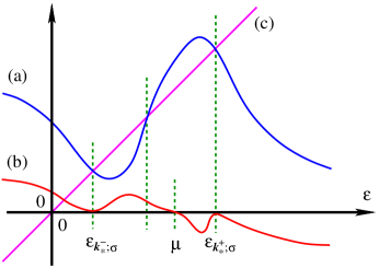
possible solutions of Eq. (4) for a given occur
in pairs (for a more precise specification see footnote ** ‣ § 3. Generalities
below), of which one is associated with point and one
with point where and are
infinitesimally close to (see Fig. 1). This
aspect, which is universally neglected in the literature for
(see however [18]
and specifically [9]; see also footnote ∥ ‣ § 2. Preliminaries above),
attains an extraordinary significance in cases where the
above-mentioned is located at some finite distance from
(considering for the moment metallic
GSs), and hence our explicit reference to in § 1
(see Eq. (15) below). This aspect will be fully clarified
in § 3.2 below.
3.2. Regular and singular contributions
to the single-particle spectral function
In anticipation of our following discussions and in view of
Eq. (5) it is instructive to introduce a decomposition
of in terms of its regular
(‘incoherent’) and singular (‘coherent’) parts. To this end, let
denote a wave vector at which is singular (not necessarily discontinuous). For
, where
are infinitesimally close to and whose
distinction is implicitly determined through Eq. (11) below
and the accompanying conditions , one can write
(10)
where () stands for a regular (singular) ‘function’ of
; for coinciding with a regular
point of , would be identically vanishing. We point out that
the equality in Eq. (10) is between two distributions
(as opposed to functions) so that it applies in some space
of test functions. In the event that
is discontinuous at , in the simplest case
******
In general, one may have
where, for the same reasons that (Eq. (12)),
and
are interdependent.
As considerations involving only unnecessarily
complicate the analysis, in this paper we explicitly deal with
cases where .
one has
(11)
where ,
(for the latter see the text following Eq. (13) below), and
(12)
The strict equality on the left-hand side (LHS) of Eq. (12)
(whereby in the subsequent parts of this paper we denote
by )
follows from the normalization condition
(13)
which applies for all, including
and . We point out that
and
satisfy Eq. (4)
for and
respectively (see Fig. 1) and, moreover, the expression
for in Eq. (11) is
specific to cases where is continuously differentiable with respect to
in the neighbourhood of (cf.
Eq. (89) below); see [18].
The normalization condition in Eq. (13) in combination
with the defining equation for in
Eq. (3) imply that
(14)
As is evident, the discontinuity of
at requires that
, for otherwise
would not have any impact on
the behaviour of , defined according
to Eq. (3). On the other hand, the discontinuity of
at implies
discontinuity of at , which, following Eq. (14), can only
materialize if the condition is satisfied [9].
Since for located at some finite (i.e.
non-vanishing) distance from the
solutions and
differ by some
finite amount
*†*†*†
Since by the arguments presented in the text following
Eq. (14) we have
, it follows that
in the event that
and would
differ only by an infinitesimal amount,
would either be a point of or
infinitesimally close to it.
(see §§ 4.2 and 4.3 as well as Fig. 1), it is of
crucial importance that particular attention is given to the
superscripts and in which as a matter of habit one is apt to ignore. We
shall elaborate on the single-particle energies
and the relationship
between these and in § 3.5
where we are equipped with the details necessary for this task.
Suffice it for the moment to mention that the single-particle
excitation energies of single-band models can be viewed as
consisting of at least (see footnote ** ‣ § 3. Generalities) two branches,
conveniently denoted by with
and
. The energy dispersions
dealt with in this paper
are ‘caricatures’ of which,
however, when continuous at the points of discontinuity of
(see § 3.4), coincide with
(cf. Eqs. (30)
and (33) below). From this perspective, it is more
transparent to denote by
. In this paper we shall
therefore alternately use the following convention:
(15)
We emphasize that, for a general , Eq. (4) has
no solution so that, in general ,
or , should be considered in
the manner specified in § 3.1.
From Eqs. (10) and (11) and the condition
which implies for
, for cases where is discontinuous at one obtains
(16)
From this result as specialized to
and Eq. (5), for interacting systems we immediately obtain
(17)
This result is of experimental significance, as the possible
singular contribution to is not capable of being resolved in real experiments.
It is also of significance to our subsequent considerations as it
shows that, for sufficiently close to , there is no restriction on the actual shape of the
corresponding in order for the
expression on the RHS of Eq. (2) to amount to a reliable
description of the dispersion of the low-lying single-particle
excitations in interacting systems, this in surprising contrast
with the heuristic arguments in § 2 that initially motivated our
introduction of the expression in Eq. (2). For illustration,
assuming that is discontinuous at
and denoting by
, from Eqs. (3), (10)
and (11) we obtain the following relationship:
*‡*‡*‡
With reference to our remark in footnote ** ‣ § 3. Generalities, we note
that for cases where has the more
general form as presented in that footnote, the counterpart of the
result in Eq. (18) would in principle differ from
that which stands in Eq. (18). However, the
considerations in § 3.6 demonstrate that the
corresponding to can
at most be equal to unity. In other words, Eq. (18) is
more general than the simple form for
in Eq. (11) would suggest. For completeness, in
Eq. (18), , , where
is the unit vector normal to
at ,
pointing from the inside to outside the Fermi sea.
A result that proves considerably useful in our considerations
in this paper is based on some simple observations. Let
(19)
and assume that is discontinuous at so that
, where
(20)
in which and are infinitesimally close to . Assuming to be continuous at ,
i.e. , one readily deduces that
(21)
where
(22)
Note that, according to Eq. (21), unless ,
discontinuity of at implies that of
at , that is . A number of applications
of the result in Eq. (21), with remarkable consequences,
will be encountered in the following sections.
Another result that will prove useful to our later analysis
concerns a situation in which as defined in Eq. (19)
is discontinuous at , similar to and . Let
(23)
Through some straightforward algebra one obtains
(24)
One observes that the requirement immediately
leads to the result in Eq. (21).
3.4. Possible discontinuities in
and
Some of the crucial results in this paper rely on the condition
of continuity of at such points
as where is
discontinuous. Here we investigate whether the two conditions can
be compatible. To this end we introduce , defined as (see Eq. (54) below)
(25)
It can be easily shown that
and satisfy the following exact relationship
[9, 10]
(26)
where stands for the
Hartree-Fock self-energy.
Let now be discontinuous at
. With
(27)
where is the nearest of the two points
and to and (by assumption) ,
from Eq. (26) we readily obtain
(28)
(29)
For metallic states, where and
are up to infinitesimal corrections equal to
for [9, 10], the LHS of
Eq. (28) is vanishing for so that, by the arguments presented in
[9], Eq. (28) establishes the continuity of
and
at (see also § 4.1).
For at a finite distance from , the LHS of Eq. (28) is strictly positive
(see footnote *† ‣ § 3. Generalities), from which and from Eq. (28) it
follows that at least one of the two functions
and must be discontinuous at .
For sufficiently close to ,
on account of the aforementioned continuity of and at all points of
and on account of the fact that these
functions are required to achieve the value at
the latter points, it is most likely that, for a possible discontinuity
of at ,
one has and that, for a possible
discontinuity of at , . Raising the status of
these observations to facts, an inspection of the signs of the terms
on both sides of Eq. (28) reveals that the possibility of
a continuous and discontinuous
at
is ruled out; in contrast, a similar inspection reveals that a
continuous and discontinuous
at is
potentially feasible. On the same grounds, it is in principle
possible that both and
are discontinuous at although, in such an event, is required to undergo a larger amount of discontinuity
(as implied by Eq. (28)) than is necessary for the case
in which is continuous at
.
It is interesting to point out that the energy dispersion as
measured by Zhou et al.[3] corresponding to
(La2-xSrx)CuO4 in the extreme underdoped limit, where
, appears to exhibit a finite amount of discontinuity at
. On identifying the measured energy
dispersion with , it is observed
that it indeed satisfies the relationship
suggested above on
general grounds.
3.5. On the points where
(and )
In our above considerations we have been able to deduce a number
of properties associated with and
by specifically relying on the property of continuity of
at (see § 3.4). Here we
explicitly assume to be
continuous also at ,
specifically at where is discontinuous; following the analysis in § 3.4,
must therefore by necessity be
discontinuous at . Let the latter
be further located inside the Fermi sea of the GS
of the system under consideration; for the ensuing discussions it is
not necessary that this GS be metallic. The general expression
for can be cast into the form
(see Eq. (21) above), with
here identified with , with the numerator of
the expression on the RHS of Eq. (2) and with the
denominator (and thus with ).
From this and Eqs. (10) and (11) it follows that
is to be identified with and with
, so that by Eq. (21) we have
the following exact result:
*§*§*§
With reference to our remark in footnote ** ‣ § 3. Generalities, we
point out that Eq. (30) is specific to cases in
which .
(30)
where is the exact
solution of Eq. (4) and, as mentioned above,
a point of discontinuity of at which,
moreover, is explicitly assumed to
be continuous. Equation (30) is to be contrasted with the more
specific exact result in Eq. (5) above. In this connection we
should point out that the validity of Eq. (5) does not
depend on whether is discontinuous at
.
This suggests that the validity of Eq. (30) may similarly
not depend on the assumed discontinuity (as opposed to the more
general condition of singularity) of
at the under consideration; at the time
of writing this paper, we are not in a position to make a definite
statement on this aspect. In this connection note that in general
is singular (not necessarily
discontinuous) for all[9, 10].
It is interesting to note that in cases where is, similar to , discontinuous
at , application of Eq. (24) followed
by some trivial algebra yields the following exact expression
(31)
from which one recovers the result in Eq. (30) for
approaching
. In cases where
, implying thus , from Eq. (31) it follows that
.
In the light of the results in Eqs. (5) and (30), it
is important to point out that, for Fermi-liquid metallic states
of the single-band Hubbard Hamiltonian (if such states at all
exist), we have shown [9] that the gradient of the
quasi-particle energy dispersion
(or the Fermi velocity times ) for inside the
Fermi sea and in the close neighbourhood of differs from by a multiplicative constant, , which we
have shown [9] to approach unity
*¶*¶*¶
In [9] for isotropic Fermi-liquid metallic states of
fermions of bare mass interacting through a short-range
potential we have obtained , where stands for the
renormalized (or effective) mass. For the sole purpose of illustration,
making the assumption that and employing the data concerning
and , corresponding
to the Coulomb-interacting homogeneous electron-gas system, as
presented in respectively Tables 5.6 and 5.7 of the book by Mahan
[23], from
for we obtain: [exact], ,
, and . Here stands for
the dimensionless Wigner-Seitz density parameter, with corresponding to the uncorrelated limit.
on reducing the on-site interaction energy . It follows that in
general the validity of (30) does not extend beyond the
points where is discontinuous;
in other words, in general the asymptotic series expansions of
and centred around a , say ,
at which is discontinuous (so that
satisfies
Eq. (4) at ; see § 3.1), only
agree to the leading order and deviate at higher orders in
; analogously for and in the event that
is continuous at (see however the last but one paragraph in
§ 3.4). This aspect becomes clearly evident by considering
the two-body interaction potential to be the long-range Coulomb
potential. In this case, is logarithmically divergent for approaching
the points of discontinuity of (see § 4;
see also [10]), a property that may or may not be shared by
; for
instance, for Fermi-liquid metallic states, is by definition [18]
bounded, satisfying
(32)
The fact that the two important points that feature in
the experimental observations as reported in
[3, 4, 5, 6, 7, 8], namely the nodal Fermi
point and , are
relatively very close to one another (typically,
amounts to approximately
% of ), implies, following
Eqs. (5) and (30), that the fundamental distinction between
and
must be of minor observational consequence for inside the
interval between and
along the diagonal direction of the 1BZ compared with outside. In other
words, in the light of Eqs. (5) and (30), it is expected
that, for inside the latter interval (between
and ),
and
should to a good approximation coincide. In the specific case at hand,
where one of our main conclusions drawn from the experimental
observations in [3, 4, 5, 6, 7, 8], specifically
those by Zhou et al.[3], is that the underlying
is continuous at the nodal points of
the Fermi surfaces of the compounds studied (see § 4.1), the
above-mentioned differences between
and should be minimal for
in the close neighbourhoods of the nodal Fermi points.
Concerning the ‘universality’ in the nodal Fermi velocities as observed
by Zhou et al.[3], since in all cases (whether
different cuprate compounds are concerned or a specific compound at
different levels of hole doping) the corresponding Fermi energies are
chosen as the origin of energy, it follows that the above-mentioned
universality of the nodal Fermi velocities is indicative of the
universality of the energy difference , where . This in turn is
suggestive of the possibility that the root cause of the discontinuity
in at should
be external to the electronic degrees of freedom, such as longitudinal
optical phonons which have been suggested [5, 8] as
inducing the ‘kink’, or ‘break’, in the observed single-particle
energy dispersions in the investigated cuprates. For an extensive
discussion of this aspect see § 5 where we argue that, whereas phonons
may be vital in bringing about the observed ‘kinks’ in the energy
dispersions, they cannot be the immediate cause but possibly a
secondary determinant through their modification of the electronic
states in such a way that is rendered
discontinuous at inside the underlying Fermi
seas and that is close to
to meV. It is important to point out that, with the exception
of rigid parabolic bands, all rigid tight-binding bands
give rise to relatively strong variation of the bare mass of fermions
as a function of doping; such variation has undoubtedly consequences
for the corresponding dressed mass and thus the interacting Fermi
velocity which, in such cases as considered here, can be artificial
and undesirable. The experimental observations by Zhou et al.[3] are thus suggestive of the possibility that rigid
tight-binding bands may not be appropriate (specifically) while
dealing with the cuprate compounds. The unsuitability of rigid
tight-binding bands (as well as rigid on-site interaction energies)
in general is the essential argument underlying the dynamic Hubbard
model proposed by Hirsch [24] (see also [25] and the
references therein) and their shortcomings specifically in
applications concerning the cuprate compounds has been explicitly
emphasized in [9].
For completeness, in cases in which
is continuous at where is discontinuous (so that, by the observations in § 3.4,
must necessarily be discontinuous
at ; see however the last but one paragraph
in § 3.4), from Eq. (25) and the application of the result
in Eq. (21) we have (see Eqs. (15) and (30))
(33)
By relaxing the condition of the continuity of
at ,
along the same lines as those leading to Eq. (31) we obtain
(34)
from which Eq. (33) is recovered for
approaching
. In cases where
, implying thus , from Eq. (34) it follows that
.
The results in Eqs. (30) and (33), which cannot
simultaneously hold (see § 3.4), gain special significance by
realizing the fact that and
correspond to a single-particle
spectral function
introduced in [9, 10], defined for all as
follows
(35)
In [9, 10] a number of salient properties of
have been explicitly
demonstrated. For instance, on replacing by in
the expression for the total energy of the GS of the interacting
Hamiltonian , one obtains exactly the same value, that is
the exact GS total energy. Although in [9, 10] was associated with
some fictitious particles, having some direct significance to the
properties of the single-particle excitations in the neighbourhood
of , Eqs. (30) and (33)
unequivocally show that
has special significance also for all outside
where
is discontinuous (as we have indicated earlier, this significance
may also extend to all points outside
where is merely singular and not
specifically discontinuous). With this in mind, Eq. (35)
shows that, at such points as where
undergoes a discontinuous change, this
is accompanied by an equally discontinuous redistribution of the
spectral weights of the peaks in the single-particle spectral
function centred at
and (see
Eqs. (30), (31), (33) and (34)).
Concerning the general subject of the spectral weight redistribution
in interacting systems as described by the Hubbard Hamiltonian, we
refer the reader to [26], and for related considerations
concerning specific strongly correlated systems to
[27, 28, 29]. We emphasize once more that Eqs. (30)
and (33) are local (i.e. they apply to isolated points, such
as is, and not to open domains of the
space) so that they do not imply equality of
with
at
.
3.6. On the number of solutions of the
quasiparticle equation at
corresponding to well-defined quasiparticles
In § 3.4 we have presented details which rigorously demonstrate
the continuity of for
in the neighbourhood of (see also § 4).
A corollary to this result in conjunction with Eq. (21) is
that, in cases where the
corresponding to is
not identically vanishing, one must have
(36)
This result establishes that, for , Eq. (4) cannot possess more than one solution
corresponding to a well-defined quasi-particle; that is to say, in
cases where is discontinuous at and ,
the expression for in
Eq. (11) is the most general expression.
*∥*∥*∥
With reference to our remark in footnote ** ‣ § 3. Generalities, this
implies that, for ,
.
The proof of this statement is as follows. Let , where and (the following arguments
can be trivially generalized for any number of similar terms
contributing to ). From
Eq. (36) it follows that
(37)
which, through the fact that in the case under consideration
(or ), implies that (). This
proves our above assertion. In other words, under the
above-mentioned conditions, Eq. (4) has at most one solution
at (and similarly for )
corresponding to a well-defined quasiparticle.
3.7. On the positivity and the possible
discontinuities of
The continuity of at a point,
say , implies that, for to be continuous at this point, it is necessary and
sufficient that the first term in the second expression on the RHS
of Eq. (8) be continuous at . The
continuity of the latter term at in cases
where is discontinuous at , following the results in Eqs. (21) and
(30), implies that, for to be continuous at , one
must have
(38)
This result is in contradiction with the fact that, for interacting
systems, (see § 2).
It thus follows that our assumption with regard to the continuity
of both and
at ,
where is discontinuous, must be false.
We thus arrive at the general conclusion that, at points (which may
or may not be points of ) where
is discontinuous, and
cannot both be continuous; at where
is continuous (see § 3.4),
must be discontinuous in cases where
is discontinuous.
§ 4. Detailed considerations
4.1. The interacting Hamiltonian and some
basic details
We consider the following interacting Hamiltonian:
(39)
where
(40)
(41)
In Eq. (39), (which has the dimension of energy)
is the coupling constant of interaction,
is a spin-degenerate single-particle energy dispersion (which may
or may not be isotropic), and
are the canonical creation and
annihilation operators respectively for fermions with spin index
, is the Fourier transform of the two-body
interaction potential (assumed to be isotropic),
and is the volume of the (macroscopic) -dimensional
hypercubic box occupied by the system. The wave-vector sums in
Eqs. (40) and (41) are over a regular lattice (the
underlying lattice constant being equal to ) covering in
principle the entire reciprocal space. On effecting the
substitutions
(42)
and restricting the wave-vector sums to wave vectors
uniformly distributed over the 1BZ associated with the Bravais
lattice spanned by ,
the Hamiltonian in Eq. (39) transforms into the conventional
single-band Hubbard Hamiltonian corresponding to
the on-site interaction energy ; in cases where
and on the RHS of Eq. (41) lie outside the
1BZ, these vectors are to be identified with the vectors inside the
1BZ obtained from and through
Umklapp processes. On relaxing the replacements in Eq. (42),
while maintaining the above-mentioned restrictions concerning the
wave vectors, the Hamiltonian in Eq. (39) coincides with
an ‘extended’ Hubbard Hamiltonian.
For the -particle uniform GS of the
Hamiltonian in Eq. (39) we have [9, 10]
(43)
where
(44)
in which
(45)
(46)
We should emphasize that, although , nonetheless is defined
over the entire available space; this we have made explicit
in Eq. (43) through . We note in passing that,
similar to and following the same
techniques as employed in [9, 10, 19], for systems
corresponding to bounded , one can readily
express , as
defined in Eq. (8) above, in terms of GS correlation functions.
Along the same lines as used in [9, 10] it can be shown
*********
To this end, one has to use Eq. (18) in [10], which
holds for all , and the fact that
and , the Hartree-Fock self-energy,
are continuous for all .
that, for the set of points for which
coincides with
, the function
(47)
approaches zero for . This
observation is significant in that it shows that, for where and is generically
(but not necessarily) discontinuous, the energy dispersion
is continuous in the
neighbourhood of (see also § 3.4).
With reference to Eq. (21), it follows that, in cases where
is discontinuous at , must undergo a discontinuity
commensurate with that in at
(and indeed at any set
introduced above) for which
attains the value (see § 3.4); in appendix
A this aspect is made explicit within an approximate framework. In
what follows, unless we explicitly indicate otherwise, we assume
to be continuous for all
.
The experimental ARPES data in [3, 4, 5, 6, 7, 8]
indicate that the measured (i.e.
from our present standpoint)
behave linearly as function of
for a finite range of away from ;
focusing on the data in [3], this is the case for
varying between zero and
approximately % of for
a nodal Fermi wave vector along the
direction of the underlying square-shaped 1BZ.
With being linear in for such a relatively small interval of vectors
(excluding the neighbourhoods of the saddle points of
), we interpret the experimental observations
as implying that
(48)
where is a nodal Fermi wave vector and where
we assume to lie inside the Fermi sea. From Eqs. (43),
(47) and (48) it follows that (see Eq. (72) below)
(49)
(50)
With reference to our earlier discussions in § 3.5, we may express
the Fermi velocity
as encountered within the framework of the Landau Fermi-liquid
theory as
(51)
where is a constant of the order of unity (see footnote
*¶ ‣ § 3. Generalities). Experiments by Zhou et al.[3]
indicate that ,
or , very weakly
depends on the doping level.
The observation in Eq. (48) is of far-reaching consequence.
This follows from a combination of two facts. Firstly, on
approaching from inside or outside the
Fermi sea, the following equation has to be satisfied
[9, 10]:
(52)
where
(53)
For , defined in Eq. (25)
above, we have the following equivalent expression [10]
(54)
where, as mentioned earlier,
stands for the Hartree-Fock self-energy. It can be shown [10]
that, for , one has
Following this and Eq. (56), one arrives at our earlier
statement concerning
for , and similarly for , as is
apparent from Eqs. (55) and (47) (see § 3.4).
Let denote the open domain of wave vectors over which
is continuous. For , applying on both sides of
Eq. (26), we have
(60)
(61)
(62)
For in an infinitesimal neighbourhood of
where
and take the value (up
to infinitesimal corrections), from Eq. (60) we observe that,
for a sufficiently smooth , a possible singular
behaviour in
and is
determined by that in on the RHS of Eq. (60).
*††*††*††
Let denote the unit
vector normal to at pointing to the exterior
of the Fermi sea FSσ. Since, for in a close
neighbourhood of , one has
for and
for , one observes that,
in cases where
is divergent for , some useful information can be
immediately deduced from Eq. (60). For instance, for
cases in which the interaction potential is as long-ranged as the
Coulomb potential and is discontinuous
at , one can explicitly show that
as so that, from Eq. (60), one
directly deduces that, firstly, , ,
for
and, secondly, the balance between these diverging contributions
must be such that the resultant function on the LHS of
Eq. (60) approaches as , irrespective of whether or .
This aspect is explicitly reflected in the defining expression
for in Eq. (58) which through
Eq. (56) determines the behaviour of for . In other regions of the space
where , a possible singular behaviour in in some neighbourhood can
in principle entirely or partly be accounted for by a similar
behaviour in .
*‡‡*‡‡*‡‡
In this connection, we point out that according to Belyakov
[30] (see also [31])
logarithmically
diverges as for
pertaining to the isotropic GS of
fermions interacting through a short-range potential.
For some relevant details see § 6 in [18].
The above observations will prove useful in our subsequent
considerations below.
For the interaction potential identified
with the long-range Coulomb potential (or a potential as
long ranged as this), it can be shown that, so long as
, in consequence of
on the RHS of Eq. (58),
for (i.e. for
approaching from inside the Fermi
sea), one has
(63)
where stands for some constant
vector. The combination of Eqs. (48) and (63) implies
that, to leading order in for
, one has according to
Eq. (56)
(64)
and consequently
(65)
Since corresponds
to the peculiar condition , for all
(see Eq. (3) above), we discard the condition in Eq. (63)
for being unphysical in the present context where Eq. (48) is
held as valid on account of experimental observations. It thus follows
that, for the case of Coulomb-interacting particles, cannot be positive, whereby Eq. (63) is rendered
obsolete. Assuming to be positive but
relatively small, it is not inconceivable that, for sufficiently
close to ,
behaves similarly to as presented
in Eq. (63) which experiments by Zhou et al.[3]
may not have resolved. Consequently, at this stage the possibility of
Eq. (63), and thus of ,
cannot be unequivocally rejected. We point out that here we are
relying on our standpoint that experimentally one measures
rather than the ‘solution’ to
Eq. (4). For completeness, in [10] (§ 6.1.3) the
consequences of satisfying an
asymptotic relation similar to that in Eq. (63) have been
investigated in some detail. In [10] (§ 6.1.3) it has been
emphasized that, for fermions interacting through the long-range
Coulomb potential, Fermi-liquid metallic states belong to the
category of states for which, as ,
satisfies Eq. (63) and fulfils a
functionally similar expression.
We conclude that the assumption of the validity of Eq. (48)
can be compatible with a picture of fermions interacting through the
long-range Coulomb potential (or a potential as long ranged as this)
only if . This condition is satisfied
(not exclusively) within the framework where the normal metallic states
of the copper-oxide based superconductors along the nodal directions
of the 1BZ are of a marginal Fermi-liquid type [32]. This
viewpoint enjoys direct experimental support through the angle-resolved
photoemission experiments by Valla et al.[4] along
the nodal directions of the 1BZ concerning the optimally-doped compound
Bi2Sr2CaCu2O8+δ.
The experimental results by Zhou et al.[3] further
show that, at , with approximately % of
,
is singular, the singularity appearing to be a discontinuity in the
slope of in the overdoped
regime and some stronger singularity in the underdoped regime. The
strongest singularity that can be expected from is a discontinuity (see § 3.4), followed by (in the
order of significance), for two-body interaction potentials as
long ranged as the Coulomb potential, a logarithmic divergence in
for
approaching the points of discontinuity of .
We believe that the observations by Zhou et al.[3]
are highly supportive of the viewpoint that, at least in the underdoped
regime, the long-range of the Coulomb potential can be of considerable
significance in determining the (unconventional) physical properties
of these compounds. For clarity, for the hole doping fraction
concerning (La2-xSrx)CuO4 (LSCO), one observes a behaviour
in the measured energy dispersion [3] which is reminiscent
of a discontinuity superimposed by a contribution whose gradient
is logarithmically divergent at .
4.2. On the relationship between
discontinuities in and
Here we demonstrate that singularity (not necessarily discontinuity)
of at a point is directly reflected in
the behaviour of
at the same point. We shall explicitly consider the case where
is discontinuous in the interior of
FS; concerning the
behaviour of
for , this is implicit in our earlier work [9, 10]
which for completeness we recapitulate in the following. In this
connection, note that is always singular
(not necessarily discontinuous) on [9, 10].
For , and attain the value
(up to infinitesimal corrections) so that the
exact inequalities and
[9, 10] imply that,
for a smooth function of in the
neighbourhood of , it is required that
undergo at least
†*†*†*
This aspect is related to the restriction for the
parameter introduced in [9];
is excluded for cases where .
a discontinuous change for transposed through
from infinitesimally inside to
infinitesimally outside the Fermi sea. For instance, for a specific
class of uniform metallic GSs of the single-band Hubbard Hamiltonian
(to which class the Fermi-liquid GSs belong) we have earlier shown
[9] (see Eqs. (105) and (106) herein) that, with
denoting the outward unit
vector (pointing from inside to outside the Fermi sea) normal to
at
one has
In [9] it has been shown that the stability of the
GS under consideration requires that
(69)
where
(70)
From Eqs. (67) and (66), one observes that on
crossing (from inside to outside the Fermi
sea), indeed the derivative of with respect to
in the direction normal to
undergoes a discontinuous change (this amounts to ),
from the positive value at to the negative value at . Similar
behaviour is shared by the pertaining to systems
of fermions interacting through two-body potentials of arbitrary range.
An analogous discontinuity takes place in
on transposing through .
For Fermi-liquid metallic GSs of systems in which the two-body
interaction potential is of shorter range than the Coulomb potential,
the functions and
are such that, on transposing
from inside to outside the Fermi sea, the continuous and
differentiable extension of
coincides with in the close
neighbourhood of (see Fig. 3 in
[9]). On the basis of this fact and a number of available
numerical results, in [9] we arrived at the conclusion that,
in the case of the single-band Hubbard Hamiltonian described in terms
of the nearest-neighbour hopping integral and the on-site interaction
energy , the corresponding and
fail to posses the latter property
for (see footnote ‡* ‣ § 5. Summary and discussion below).
Having described the singular behaviour of in the neighbourhood of ,
we now set out to demonstrate that a discontinuity in
at (i.e.
is strictly located in the interior of the
Fermi sea FSσ) gives rise to the following result:
We present the proof of the result in Eq. (71) in § 4.3
below. Note that .
††††††
It is important to realize that, in contrast with the case where
a possible discontinuity in at
corresponds to (see
Eq. (18)), there is no a priori restriction
on the sign of (viewed as the value of
and not as spectral weight) for
outside . This is appreciated by
realizing the fact that all excitations corresponding to the
wave vector outside can, by the very definition of ,
only correspond to many-body states whose energies are greater
than the energy of the GS of the system under consideration, whereby a
possible negative cannot signify
an instability of the latter GS. This aspect is already reflected
in the fact that, for located at a finite distance
from , the choice of what we denote by
and is in principle arbitrary.
That in our present considerations ,
is related to the fact that we have chosen to
be the closer of the two vectors and
to the nodal Fermi point and that, in order for ,
or , to attain the required value
at , it
must (monotonically) increase for transposed from
to .
For two-body interaction potentials of shorter range than the
Coulomb potential, ; therefore, on account of
Eq. (71), one has
(74)
Introducing, in analogy to the problem of electrons coupled to
phonons [23] (see specifically § 6.4 herein), the
‘mass-enhancement factor’ as follows
The result (specifically
) conforms with the experimental
observations concerning the cuprate compounds [8] (see
Fig. 4 herein where is what here we have
denoted by ) (see also [33]).
For we have
†‡†‡†‡
We point out that the significance of as the
subscript of lies in the
finite difference between (which lies strictly
below ) and (which lies strictly above
) for located at some finite distance from
(see § 4.3) and not in the
possibility that is a discontinuous
function of at . In view of the
latter, we should emphasize that far from dismissing a discontinuity
in , at ,
as being a priori infeasible, our statement here only reflects
the confines of our considerations in this paper. We hope to return
to this subject matter in a future publication.
(77)
whose existence depends on the existence of the second term
in parentheses on the RHS of Eq. (77). In this
connection it is important to realize that a finite positive
is not sufficient for the last
term in Eq. (77) to be bounded. With reference to the
convention adopted in Eq. (15), we write
(78)
In a similar fashion,
(79)
For Fermi-liquid metallic states where
is discontinuous at ,
and are
collinear and point in the same direction for all. For the uniform GSs of the single-band
Hubbard Hamiltonian, in [9] strong evidence is presented
indicating that for , and , , are not collinear so that these states
cannot be Fermi liquids (see also footnote ‡* ‣ § 5. Summary and discussion below).
Assuming to be non-zero
and bounded, from Eq. (71) it follows that differs from for any arbitrary vector
outside the plane normal to . Let denote the outward
unit vector normal to at
, with
the point at which the extension of the
radius vector meets .
For inside the Fermi sea and sufficiently close
to , the inner products of the three
vectors in Eq. (71) with
are all non-negative so that on account of Eq. (71) in
general we have
(80)
The discontinuity in at , where by assumption
is discontinuous, is seen to show the same trend as observed in the
experimental results by Zhou et al.[3] (and other
workers [4, 5, 6, 7, 8]). To clarify this aspect,
we point out that, by Eq. (5),
and coincide at . Following Eq. (30), whose validity
depends on the discontinuity of and
continuity of at , and
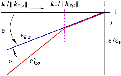
also coincide at . This situation is schematically illustrated in
Fig. 2 where the distinctions between the two energy
dispersions is depicted as being minute over the entire interval
between and along a
nodal direction of the 1BZ. With this picture in mind, the conformity
of the result in Eq. (80) (and indeed Eq. (71)) with the
experimental results by Zhou et al.[3] (excluding
those corresponding to underdoped samples) becomes evident.
A convenient (though not necessarily an exact) representation of
Eq. (71) in terms of two angles and is
obtained as follows. We take the inner product of both sides of
Eq. (71) times with and multiply both
sides of the resulting expression by
(81)
so as to obtain a relationship between dimensionless quantities.
Assuming
to be small, for similarly small
one
can consider as being a linear
function of , passing, along the nodal direction of the
1BZ, through the point at angle with respect
to the wave-vector axis (see Fig. 2), where
(82)
Here , following the convention of counting
angles as positive when they imply counterclockwise rotation
with respect to point in Fig. 2. Following
Eqs. (5) and (30), to a good approximation
should be equal to in the interval between and the nodal
Fermi point ; in the case of particles
interacting through the long-range interaction Coulomb potential,
the agreement between and
in the neighbourhood of is the better the smaller the value of
, ideally when (see § 4.1). For satisfying , and depart according to Eq. (71). Since this aspect
is a direct consequence of (see
Eq. (71)), it follows that in the neighbourhood of the behaviour of
in relation to very crucially depends
on the range of the two-body interaction potential. In view of the
experimental results obtained by Zhou et al.[3], we
believe that the influence of the long range of interaction on
is unequivocally present for samples
in the underdoped regime; for the samples in the optimally-doped
and overdoped regimes, this aspect is not as unequivocal as in the
case of the underdoped samples. It is reasonable to believe that this
feature has its root in the magnitude of
which for an increasing level of (hole) doping should be decreasing,
rendering thus the influence of the long range of the two-body Coulomb
potential at less effective. In order to
maintain a non-vanishing amount of discontinuity in at , however, following
Eq. (71), the decrease in should
be accompanied by a concomitant decrease in in such a way that the rate of decrease
in
(this decrease is evident from the the experimental results
in [3]) for the increase in the level of hole doping is
not as strong as would be the case for a doping independent
.
For an interaction potential of shorter range than the Coulomb
potential, it is expected that the behaviour of is semilinear
†§†§†§
That is, it is linear, but its extension does not pass through the
‘origin’ in Fig. 2. As we shall discuss in
some length in § 5 below, interestingly the experimental energy
dispersions in Fig. 1a of [3], when linearly
extrapolated from the region (i.e.
at ‘high’ binding energies) to ,
all turn out to meet the energy axis at meV above the Fermi
energy .
for sufficiently small values of in the
region . This semi-linear line
stands at angle with respect to the linear line depicting
in Fig. 2, for which we have
(83)
(84)
Here , following the convention stated above in
connection with in Eq. (82).
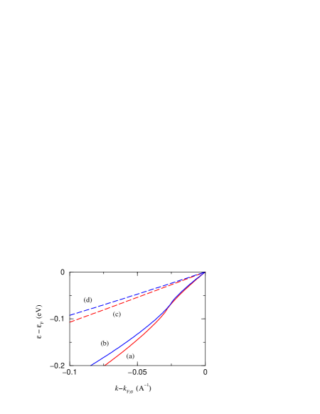
In Fig. 3 we present results concerning
within an approximate framework
in which has the functional form of the
Hartree-Fock self-energy (see appendix A; Eq. (A33)),
evaluated in terms of a momentum distribution function
which is continuous at the nodal
Fermi point and discontinuous at
. The results in Fig. 3 concern
a planar square-lattice model (for the relevant parameters see
the caption of the figure) and the two solid curves correspond to
two densities of particles representing the underdoped and
overdoped regions of the hole-doped cuprates. We obtain almost
identical results as in Fig. 3 by employing an isotropic
model defined on the continuum and for one, two and three spatial
dimensions;
†¶†¶†¶
With and
(for the
specification of the quantities encountered here, see the caption
of Fig. 3), we have employed the following
:
For ,
;
for ,
;
for ,
, where is the
exponential-integral function and is a constant parameter
of dimensions of reciprocal metre.
our observations concerning are particularly relevant in light
of the fact that in the superconducting state, or in the advanced
stages of the pseudogap phase, the experimental observations along
the nodal direction of the 1BZ should be influenced by the reduced
wave-vector space available to gapless excitations. Not surprisingly,
our numerical calculations for reveal that similarly all
qualitative aspects of the results in Fig. 3 remain intact
by modeling in such a way that the
discontinuity in is anisotropic, taking
its maximum value at along the diagonal
directions of the 1BZ and diminishing for directions away from the
diagonal directions.
Considering the fact that, in real materials, charged fermions interact
through the long-range Coulomb potential, the experimental results by
Zhou et al.[3], as well as those by other workers
[4, 5, 6, 7, 8], should be viewed as consisting of
a superposition of the results in Figs. 2 and 3; here
we are leaving aside the possibility of a discontinuity in
at which
is theoretically feasible (see § 3.4) and appears to be realized in
the underdoped (La2-xSrx)CuO4[3], specifically
at .
4.3. Explicit calculation of the amount of
discontinuity in
at , with
Here we present the details underlying the derivation of the
result in Eq. (71) above. For definiteness, unless we
explicitly indicate otherwise, throughout this section we assume
to be continuous at where is considered
discontinuous (see § 3.4).
The expression for as presented
in Eq. (43) is not suited for the determination of
, on account
of the fact that Eq. (43) describes in terms of a distribution (i.e. ; see text following Eq. (10) above) while the
available algebraic machinery required in our approach is effective
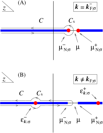
for functions. To proceed we therefore define
(85)
in which the contour has been depicted in Fig. 4.
For definiteness, we consider to initiate and terminate
at the point of infinity in the complex plane, corresponding
to in Eqs. (6) and (7). It can be readily
verified that
(86)
(87)
Making use of these results, from the defining expression in
Eq. (43) we have
(88)
This expression has the generic form of defined in
Eq. (19) so that, in determining the amount of possible
discontinuity in , we shall rely on the result in Eq. (24).
We assume to be discontinuous at
. In what follows we consider the case
in which lies strictly inside the Fermi sea, that
is at a non-vanishing distance from . On
account of the assumed discontinuity of
at , following Eq. (30) we can
replace on the RHS of
Eq. (88) by .
†∥†∥†∥
With reference to our remarks in footnote ** ‣ § 3. Generalities,
here we are implicitly assuming that .
The assumption with regard to the discontinuity of at implies that
is bounded in the neighbourhood
of (similarly
for in the neighbourhood of
(see
Fig. 1)). Consequently, for in the neighbourhood
of we can write
(89)
(90)
where (not to be confused with
introduced in Eq. (44) above)
is a function which is bounded at and
denotes a function
which asymptotically is subdominant with respect to
for . In Eq. (89),
denotes the analytic continuation of
into the physical Riemann sheet
of the complex plane, from which
is obtained according to , . It is trivially verified that
(91)
In our subsequent
considerations we assume
to be bounded for in a neighbourhood of
(see Eq. (114) below). For
discontinuous at and in a
neighbourhood of , we employ the decomposition
where
; the
contour consists of the union of two semi-circles
of infinitesimal radius centred at on the real axis of the complex plane (see
Fig. 4). Thus we write
(92)
where and are the contributions due to contours
and respectively. The decomposition of
according to Eq. (92) can be viewed
as arising from the decomposition of
in terms of its regular and singular contributions, as presented in
Eq. (10) above. Following our considerations in §§ 3.1 and
3.2, for at which Eq. (4) has no solution in the
interval , is
identically vanishing.
From Eq. (88), making use of the general result in
Eq. (24), we have
†**†**†**
Below (as well as elsewhere in this paper) in
denotes left/right gradients of , defined as the
limit of for
approaching from the left/right; here
left/right is defined by . For the definition
of see text preceding
Eq. (80) above.
(93)
(94)
(95)
(96)
In arriving at Eq. (93) we have made use of the assumed
continuity of in a neighbourhood
of , implying, in conjunction with the
assumption of discontinuity of at
, the equality of
with
(see Eq. (30)).
The subsequent notation will be considerably simplified by
introducing the following decomposition
†††††††††
Note that here
,
, stands for an entire symbol, that is
does not on its own denote
an independent operation.
(97)
where
(98)
and
(99)
In this way, making use of
(100)
Eq. (93) can be written in the following equivalent form
(101)
(102)
(103)
(104)
We now proceed with the determination of the terms on the RHS of
Eq. (101). It is readily verified that (see footnote †** ‣ § 4. Detailed considerations)
(105)
(106)
(107)
Following the Dyson equation, making use of Eqs. (89) and
(91), we have
From Eqs. (101), (118), (120), (122),
making use of Eqs. (92) and (98) we arrive at
(123)
which is simply the expression in Eq. (71) in disguise;
this is readily verified by employing the results in Eqs. (98)
and (99). We observe that a finite gives rise to a finite discontinuity in at (see
Fig. 2).
An important aspect of the result in Eq. (123) is the
following. In § 4.1 we have emphasized that, for metallic GSs of
fermions interacting through potentials which are as long ranged
as the Coulomb potential, logarithmically diverges for
approaching any region where
undergoes a discontinuous change [10]. Since
(124)
in follows that any logarithmically divergent contribution that
may be contributing to for , which by
necessity has the same sign for
and ,
†‡‡†‡‡†‡‡
See footnote *†† ‣ § 4. Detailed considerations. Further, for a simple model,
such as the electron-gas model, this aspect can be demonstrated
by explicit calculation.
cancel. Thus, even though for the above-mentioned systems
is
divergent for , for these
systems, following Eqs. (123) and (124),
is bounded.
Finally, we point out that Eq. (123) is not applicable
to cases in which .
This aspect is rooted in the failure of Eq. (98) for
which, in turn
originates from the fact that, on all points of , acquires its maximum
value (namely ) [9, 10]. As can be
explicitly shown, for ,
the LHS of Eq. (98) is equal to .
§ 5. Summary and discussion
In this paper we have presented a set of complementary pieces of
evidence indicating that the single-particle energy dispersions as
deduced through the ARPES are in fact
(Eq. (43)) rather than (more
precisely, ) that formally is a
solution of the quasi-particle equation (Eq. (4)). We have
shown that, in addition to
coinciding with on the Fermi surface
of metallic GSs, the two energy dispersions
are equal at any point inside the underlying Fermi sea FSσ
where the GS momentum distribution function
undergoes a discontinuous change and
is continuous; at the time of writing this paper the question remains
open whether this property is retained when the last-mentioned
discontinuity in is replaced by a more
general kind of singularity. One of the conclusions that we draw from
the analysis of the experimental data obtained by Zhou et al.[3] as well as by other workers
[4, 5, 6, 7, 8] is that (in particular), along the
nodal directions of the 1BZs of the cuprate compounds investigated
by the latter workers, is discontinuous
at a point located in the close vicinity of the nodal
Fermi point ( typically amounts to some % of
). From this and our aforementioned
finding with regard to the equality of
and at and
we have concluded that in the interval
along the diagonal direction of the 1BZ between
and the two energy dispersions
and should be in general experimentally indistinguishable
(see Fig. 2). For fermions interacting through the long-range
Coulomb potential, and
have distinct behaviours in the
neighbourhoods of points where is
discontinuous (§ 4.1). Since, according to our analyses, the
corresponding to systems studied by
Zhou et al.[3] must be either continuous or only
slightly discontinuous at , we have
arrived at the conclusion that the influence of the long-range of the
Coulomb interaction potential should be strongest at . The experimental data obtained by Zhou et al.[3] indeed show that for the underdoped sample
(La2-xSrx)CuO4, corresponding to for instance ,
the measured energy dispersion shows behaviour in the vicinity of
that markedly differs from similar energy
dispersions corresponding to optimally-doped and over-doped
samples of (La2-xSrx)CuO4. This difference can be
viewed as consisting of two separate contributions, namely a
finite discontinuity and a logarithmic divergence in the
slope of the energy dispersion at .
The former is consistent with the exact result obtained in § 3.4
according to which can undergo
a discontinuous change at points inside FSσ where
is discontinuous, and the latter
is feasible only if the two-body interaction potential is as
long ranged as the Coulomb potential. We point out that, in cases
where is discontinuous at the
point of discontinuity of , that is
, neither nor
coincides with ; here
. However, in cases
where , and thus ,
it can be rigorously shown that .
Our point of departure in this paper has been based on the consideration
that single-particle energy dispersions as measured by the ARPES
coincide with the average value of with respect to the
normalized energy distribution function ; this average value we have
denoted by . Throughout this paper
we have presented a host of evidence to support this point of view.
On the basis of this viewpoint we have proposed the standard variance
of with respect
to the above-mentioned normalized energy distribution function as
corresponding to the measured width of the peak in centred at .
From the expression for we
have inferred that sharp variations in
are directly reflected in the behaviour of . We have shown for instance that the combination of
a discontinuous and continuous
at
(whereby ) implies a discontinuity
in at
with the change in being of
the same sign as that in , that is
.
For (La2-xSrx)CuO4 at , Zhou et al.[3] observed a decrease in the electron scattering
rate (i.e. the width of the MDC) at the same energy as a
discontinuity in the gradient of the energy dispersion is observed
on transposing from ‘below’ to ‘above’ ,
corresponding to and
respectively. This decrease
in the scattering rate is in full conformity with the sign
associated with which has
to be positive in order for the change in the energy dispersion as
described by the expression deduced in this paper (Eqs. (71)
and (123)) to conform with the experimentally observed
change (see footnote †† ‣ § 4. Detailed considerations). A sudden change in the spectral width
at the energy corresponding to the ‘break’ in the single-particle
energy dispersion has also been reported in [5, 7, 8].
Since amounts to the kinetic energy corresponding to the GS of
the Hamiltonian in Eq. (39), one observes that a
finite discontinuity in in the interior
of the underlying Fermi sea, of the type indicated above, necessarily
results in a higher kinetic energy than the kinetic energy
corresponding to a comparable which,
however, is free from the latter discontinuity; in this connection,
recall that and that , independent of the the
strength of the interparticle interaction, so that a discontinuity in
over a set of points
in the interior of the Fermi sea, with , is
necessarily accompanied by a ‘spillage’ of
into the region outside the Fermi sea. We thus observe that the
interpretation as put forward in the present paper of the experimental
observations in [3, 4, 5, 6, 7, 8] also provides
a natural explanation concerning the experimental observations of
the excess ‘kinetic’ energy in the normal states of the doped cuprate
compounds [11, 12] in comparison with the ‘kinetic’ energies
of the GSs of conventional metals; in arriving at the latter statement
we have relied on the supposition that the gapless excitations along
the nodal directions of the 1BZ (below the pertinent superconducting
transition temperatures) are akin to the gapless excitations of the
normal states of the investigated cuprate compounds. Experimental
observations, at temperatures elevated above the pertinent
superconducting transition temperatures, along various directions
of the 1BZ [5] (concerning change in the spectral widths see
[8]), are in conformity with the above-mentioned supposition.
Although the considerations in this paper provide a consistent
scenario concerning the main aspects of the experimental data in
[3, 4, 5, 6, 7, 8], a fundamental question
remains to be answered, namely whether a single-band model which,
moreover, exclusively takes account of the electronic degrees of
freedom (Eq. (39)), allows for a uniform metallic GS whose
corresponding single-particle spectral function involves a coherent
contribution below characteristic of a
well-defined quasi-particle excitation at
located inside the underlying Fermi sea (i.e. at some finite
distance from ). Note that, although the
existence of a well-defined quasiparticle excitation at is sufficient for rendering discontinuous at , this
discontinuity does not necessarily imply that the pertinent excitation
energy should lie by a finite amount below the Fermi energy;
conversely, in cases where the excitation energy at issue is less
than the Fermi energy by a non-vanishing amount, it is necessary (in
fact by definition) that be located away from
(see paragraph following Eq. (14)
above). Recent Monte Carlo results corresponding to projected
variational wave functions [34, 35] concerning the conventional
single-band Hubbard Hamiltonian (involving only an on-site interaction
between fermions of opposite spin) on a square lattice, are not
supportive of the possibility of a noticeable discontinuity in
in the interior of the underlying Fermi sea.
‡*‡*‡*
It is interesting to note that the
as reported in [34, 35] (along the nodal direction
of the 1BZ of a square lattice and corresponding to a projected
variational wave function for and ) unequivocally
violates the result . Following
the analysis in [9] and in full conformity with the
conclusion arrived at herein, we observe that the underlying metallic
GS is not a Fermi liquid.
Furthermore, although for the hole-doping fraction approaching
zero, the discontinuity of at the nodal
Fermi point diminishes (according to the
authors of [34, 35], scales
like for sufficiently small ), for corresponding to optimal
doping (here ) it is relatively too large for the
following two reasons. Firstly, since , the larger the value of , the
smaller is the maximal value that , or
(see Eq. (76)), can possibly attain; following Eq. (71),
a small value for the latter quantity corresponds to a small ‘kink’
in the single-particle energy dispersion
at .
Secondly, in principle a non-vanishing (and in practice a relatively
large) corresponding to a nodal
Fermi point at optimal doping does not conform with the experimental
observations by Valla et al.[4] according to which
the self-energy in the neighbourhood of a nodal Fermi wave vector
along a nodal direction of the 1BZ satisfies the scaling behaviour
characteristic of the self-energies of marginal Fermi liquids.
Assuming that, insofar as our present considerations are concerned,
the variational results in [34, 35] are sufficiently accurate,
we have no alternative but to pronounce the conventional Hubbard
Hamiltonian (as opposed to ‘extended’ Hubbard Hamiltonians and as
opposed to Hamiltonians, such as the Hubbard-Holstein Hamiltonian
(see, e.g., [36]), in which the fermionic field is coupled
to an external bosonic field) as being inadequate for describing
the phenomena observed in [3] and
[4, 5, 6, 7, 8]. This conclusion contradicts the
finding by Randeria et al.[37] whose analysis is based
on the very same computational results (i.e. those reported in
[34, 35]) as relied upon by us above.
Concerning the interpretation of the experimental observation
in [3, 4, 5, 6, 7, 8] as presented in
[37], denoting the Fermi velocity at high binding energies by
(to be compared with what we have in this
paper denoted by ) and that
at low binding energies by (to be compared
with ), Randeria et al.[37] deduce that
(compare with Eq. (71) above) where stands for what we have
in this paper denoted by , to be strictly
distinguished from . The expression as
deduced in [37] for is the standard
expression for the Fermi velocity in (isotropic) Fermi-liquids (see
Eq. (7) in [37]). Through stating that “at intermediate to
high energies, ”,
where is the real part of self-energy as evaluated at
“”, Randeria et al.[37]
deduced an expression for which up to the
numerical factor (by the latter statement this is identified with
unity) coincides with that for and hence the
above-quoted expression relating the two velocities. It is evident
that the crucial, and in our opinion manifestly unjustified, step
taken by Randeria et al.[37] in deducing the expression
is that of effecting
the condition “” in
the expression concerning , for the essential
aspect of the experimental observations being interpreted concerns
a change in energy dispersions (or discontinuity in Fermi velocities)
over a relatively very narrow range of energies (centred around, for
instance, approximately meV insofar as the experiments reported in [3] are
concerned) whereby an appeal to the relationship
“” is seen to
be entirely unwarranted. The only possibility that would justify
an appeal to the latter relationship would be the discontinuity
of “” at , with reducing to a
nearly constant function
‡†‡†‡†
For the uniform GSs of the single-band Hubbard Hamiltonian,
which are dealt with in [37],
, where
is the number of fermions with spin index
(the index complementary to ) per site and
is the on-site interaction energy. The above-mentioned nearly-constant
function must therefore be close to the latter limiting value.
of for all. By the
Kramers-Krönig relation the imaginary part of the
self-energy would be almost vanishing for all, which is neither realistic nor enjoined by the
experimental observations under consideration. We therefore conclude
that the considerations by Randeria et al.[37] do not
shed light on the observations as reported in
[3, 4, 5, 6, 7, 8].
It is important to point out that according to a widely, but not
universally, held view (for a review see [33]; see also
[38]), both the ‘kink’ in the single-particle energy
dispersion and the decrease in the spectral width at are to be attributed to electron-phonon
interaction [8, 39].
‡‡‡‡‡‡
Concerning the role envisioned for the electron-phonon interaction
in the context of high-temperature superconductivity in the cuprate
compounds see [40] and for the interplay between
electron-electron and electron-phonon interactions see
[41].
Counterarguments, disfavouring phonons and attributing the latter
phenomena to antiferromagnetic spin fluctuations have been put forward
‡§‡§‡§
For completeness we mention that we fail to comprehend the
methodology with the aid of which the authors of
[42] deduced from their computational results
concerning the single-particle spectral function (denoted in
[42] by ) a kink in the
single-particle energy dispersion. In our judgement, connecting
the maxima of a series of corresponding to
various (considered as parameter), as the authors of
[42] did (see Figs. 4 – 6 in [42],
noting that in these is measured in milielectron volts
and in units of the inverse lattice constant), cannot
provide unequivocal information with regard to the dispersion of
the underlying single-particle excitation energies. [43, 44, 42] (see also the discussions in [6, 7]
which concern experiments as well as those in [5], examining
experimental observations in the light of a number of different
theoretical possibilities). We do not consider electron-phonon
interaction as being the primary cause for the ‘kink’ in the
experimentally measured energy dispersions. This becomes evident by
linearly extrapolating the data in Fig. 1a of [3] at high
binding energies (corresponding to energies between approximately
and eV below the Fermi energy ) towards the
nodal Fermi point . One observes
that at the extrapolated energy
dispersions corresponding to all doping concentrations (in total
energy dispersions corresponding to ) intersect
the energy axis at the same point (this with remarkable accuracy)
above the Fermi energy, namely at approximately eV
above (instead of at, or nearly at,
if electron-phonon interaction were directly at
work; see later); this excess energy is almost equal to the binding
energy (i.e. ) at which ‘kink’
in the energy dispersions has been observed. The conventional
electron-phonon theory [23] (see in particular § 6.4 herein),
according to which , where
is the coupling constant of the electron-phonon
interaction, or the electron-phonon contribution to the mass
enhancement (for a comprehensive overview see [45]),
requires that the change in the energy dispersion correspond
to a clockwise ‘winding’ around (inside
an energy window of width centred at
,
‡¶‡¶‡¶
See, for example, Fig. 26.1 in [46]; see also
Fig. 6.16 in [23] and note that the electron-phonon
self-energy is vanishing at , or
using the notation adopted in [23], at . where
the the characteristic phonon frequency) of the
electronic dispersion with respect to that in the absence of
phonons; the ‘kink’ in the single-particle energy dispersions in
systems of electrons coupled to phonons is thus seen to correspond
to a sharp crossover of the phonon-dressed dispersion into that of
electrons in the absence of electron-phonon interaction (from which
the phonon-dressed energy dispersion becomes rapidly indistinguishable)
at some short distance outside the above-mentioned energy window;
linear extrapolation of electron-phonon dressed energy dispersions
from outside the above-mentioned crossover region (and
corresponding to ) must
therefore at very nearly
intersect the energy axis at .
Experimentally, this aspect is evident from the high-resolution
photoemission data concerning the surface state of beryllium
(also referred to as the -surface state of Be) as
presented in Fig. 3 of the work by Hengsberger et al.[47] (see also [48]). A comparison of the data
in Fig. 3 of [49] with those in Fig. 4 of [48]
leads one to conclude that the above-mentioned clockwise ‘winding’
around of the phonon-dressed single-particle
energy dispersions with respect to their undressed counterparts is
also present in the energy dispersion of the surface-state
of molybdenum [49]. With reference to our above statement with
regard to the extrapolation of the energy dispersions in Fig. 1a of
[3] corresponding to
towards , it is evident that the
‘kinks’ observed in the single-particle energy dispersions in the
hole-doped cuprate compounds
[3, 4, 5, 6, 7, 8]cannot be a direct
consequence of the electron-phonon interaction.
In order to examine the possibility of an indirect role played by
phonons in bringing about ‘kink’ in the energy dispersions as observed
in [3, 4, 5, 6, 7, 8], it is instructive to
recall a model proposed by Fröhlich [50, 51] (see also
§§ 1.8 and 3.16 in [52]). Fröhlich [50, 51]
showed that, for sufficiently large value of coupling constant,
the interaction of independent electrons with phonons gives rise
to an exotic electronic GS, which Fröhlich showed to be a
superconducting state.
‡∥‡∥‡∥
Schafroth [53] has, however, shown that, as the
theory of Fröhlich is based on a finite-order perturbation theory
concerning electron-phonon interaction (explicitly, a second-order
theory), it fails to describe the Meissner effect. For an
exposition of the work by Schafroth see [52]
(appendix A1.8 herein).
In this state, the Fermi sea of electrons consists of two
concentric regions, separated by a narrow region of unoccupied
single-particle states (see Figs. 1 and 2 in [50]); Fröhlich
explicitly showed that this GS, corresponding to a ‘shell’
distribution of electrons in the space, is characterized
by the equality of the widths of the intervening unoccupied region
and the outer occupied region of the space. For such a
state, on transposing from the interior of the inner
Fermi sea to the exterior of the outer Fermi sea, undergoes three discontinuities, from unity to zero,
from zero to unity and again from unity to zero respectively. Each
of these discontinuities would in turn give rise to discontinuities
in (in principle; § 3.4) and
, in the manner
described in this paper (§§ 3.4, 4.2 and 4.3), were it not for the
fact that these discontinuities all correspond to single-particle
excitations whose energies coincide with . It
follows that the Fröhlich state is not the appropriate state
insofar as the observations in [3, 4, 5, 6, 7, 8]
are concerned. In spite of this, the crucial role that phonons play
in bringing about the Fröhlich state (at least in principle), with
the above-indicated discontinuities in the associated
, makes evident that phonons can in
principle be vital in regard to the observations reported in
[3, 4, 5, 6, 7, 8];
in this connection it should be noted that the binding energies
corresponding to ‘kinks’
in the measured single-particle energy dispersions of the investigated
cuprate compounds very nearly coincide with the energies of the
longitudinal optic phonons in these [8] (for a detailed
discussion of this subject see [33]).
We point out that the prediction by Fröhlich [50] of the
above-mentioned ‘shell’ state relies on a second-order perturbation
expansion of the GS energy of the coupled electron-phonon system. Soon
after its predication, this state was asserted by Wentzel [54]
and Kohn and Vachaspati [55] as not feasible through its
interception by a structural lattice instability at an electron-phonon
coupling constant smaller than that required for the formation of the
Fröhlich state; Wentzel [54] conceded, however, that interaction
of electrons, not taken account of in Fröhlich’s considerations,
would render the Fröhlich state feasible. However, according to
Bardeen [56] (see the closing paragraph of section III herein),
who has established a modified stability condition for the lattice,
the Fröhlich state is viable.
‡**‡**‡**
Anderson [57] presented the contents of the
Fröhlich model in a modern setting, indicating the diagrammatic
representations of the underlying exchange processes. Subsequently,
with reference to a Migdal theorem [58], Anderson
[57] stated (p. 1346): “But in fact
Migdal resolved the problem even more completely by showing that
is a much more sensitive function of than of
— i.e., it is local in space, retarded in time, thus depends
on much more sharply — so that the large correction
to comes from : …
and is always positive:
the Fröhlich-Bardeen instability simply does not occur. The
complete treatment shows that phonon instability and the first
singularity of actually occur precisely at the same coupling
strength.” Two comments are in order. Firstly, the electronic
state on which the Migdal theorem at issue is based is that of
the non-interacting free-fermion model (this is readily verified
through inspecting [58] in conjunction with
[50]); in other words, it is assumed that the scale
of the electronic excitation energies is determined by a single
electronic mass parameter. For specifically strongly-correlated
electron systems there is no a priori reason to believe that
the GS of this model would at all be an appropriate starting point
for dealing with the problem of electron-phonon interaction (this
is exactly the same problem which in fact hinders a rigorous
formulation of a theory concerning the superconducting states of
the cuprate compounds whose low-lying single-particle excitations
in the normal state are not quasi-particle-like; see however
[59]), so that the above-mentioned Fröhlich-Bardeen
instability cannot on its own rule out the existence of the
Fröhlich state. Secondly, it is generally, even though perhaps
not universally, accepted that non-adiabatic processes are significant
in the copper-oxide-based high-temperature superconductors, leading
to the ‘failure’ of the Migdal theorem referred to above. See
[60]. For completeness, we have carried out
calculations [61] on a uniform two-dimensional model
in which the GS is the Fröhlich state. From the first-order
self-energy in terms of the dynamically screened interaction
function we have deduced quasi-particle lifetimes which are
generically by one order of magnitude shorter than the lifetimes of
quasi-particles in the conventional two-dimensional model at similar
densities. We have further studied [61] a variety of
the properties of this model in the superconducting state within the
Bardeen-Cooper-Schrieffer (BCS) framework, despite the fact that the
aforementioned short quasi-particle lifetimes undermines the use of
the BCS formalism. For instance, in the weak-coupling limit we obtain
that is relatively close to (to
be compared with the conventional BCS value of ). We point out
that a recent [62] non-selfconsistent first-order
calculation (in which the effective interaction has been deduced
from diffusion Monte Carlo results concerning the static charge and
spin structure factors and random-phase approximation Ansätze
concerning the dynamical density-density and spin-spin susceptibilities)
concerning two-dimensional liquid 3He indicates that on increasing
the aerial density of 3He atoms the effective mass diverges; a
subsequent increase of the density suggests what Boronat et al.
[62] refer to as being indicative of a transition
to “anomalous occupation numbers” and to which we would refer
as the Fröhlich ‘shell’ state. Interestingly, according to Boronat
et al. [62] “Both spin and density
fluctuations have profound effects.”
Concerning the ‘universality’ (within an experimental uncertainty
of approximately %) of the Fermi velocities at low binding
energies as reported by Zhou et al.[3], following
the analysis in § 3.5, this ‘universality’ reveals two aspects;
firstly, the ‘universal’ energy , where , is associated with
some bosonic excitations that are external to the electronic
degrees of freedom, supporting the possibility that longitudinal
optical phonons, though not directly (see above), can
indirectly be the sought-after bosonic excitations; secondly, a
rigid, that is doping-independent, tight-binding energy dispersion
underlying the many-body Hamiltonian in
Eq. (39), is not capable of reliably describing the
cuprate compounds, specifically those investigated by Zhou et al.[3]; the bare mass corresponding to a rigid tight-binding
energy dispersion is relatively strongly dependent on the level of
doping (see caption of Fig. 3), and this is most likely
inherited by the corresponding dressed mass and consequently the
interacting Fermi velocity, thus contradicting the above-mentioned
experimental observations.
Although in this paper we have mainly focused on the ARPES data
along the nodal directions of the 1BZs of the cuprate compounds
as reported in [3, 4, 5, 6, 7, 8], our approach
is applicable along any direction of the 1BZ. In the light of the
observations as reported in [5] (see specifically
Fig. 3 in [5]) we conclude that a discontinuity in
in the interior of the Fermi sea may
be a generic property of the normal states of all cuprate
superconductors. With reference to our observation in this paper
that along the nodal directions of the 1BZs of the cuprate compounds
investigated in [3, 4, 5, 6, 7, 8], the
quasi-particle equation must have at least (see footnote ** ‣ § 3. Generalities)
two solutions
and
corresponding to true Landau quasi-particles (in the sense of
), it is interesting to recall
an earlier observation presented in [9]; here it has
been rigorously shown that, within the framework of the conventional
single-band Hubbard Hamiltonian, for located in the
pseudogap regions of the reciprocal space, the quasi-particle
equation must have (at least) two solutions, one strictly below
and one strictly above , and that these solutions do
not correspond to quasi-particle excitations of the Landau type,
but to resonances. It is of interest to investigate whether, and
if so, how these two distinct energies are related to
and
which correspond to Landau
quasiparticles. We should emphasize that, whereas the above-mentioned
resonances correspond to wave vectors in the pseudogap regions of the
underlying putative Fermi surfaces (in [9] it has been
shown that
ࠠࠠࠠ
Here stands for the Fermi
surface corresponding to ,
in which has been chosen such that
the interior of contains the
same number of points as contained in the interior of
, namely , the total
number of fermions in the GS with spin index . , which may or may not be empty,
constitutes the pseudogap region of the wave-vector space), the
wave vector is located in the interior of
Fermi seas, i.e. at some finite distance from
.
We close this section by reiterating that, although we have been
able to provide a consistent scenario for the experimental
observations in [3, 4, 5, 6, 7, 8], a number of
outstanding questions remain. These are
(i) whether a single-band model is capable of possessing a uniform
metallic GS whose momentum distribution function is discontinuous
in the interior of the underlying Fermi sea (specifically along the
nodal directions of the 1BZ) and at the pertinent wave vector,
denoted in this paper by , the single-particle
spectral function involves a singular contribution at where lies some
to meV below the Fermi energy ,
(ii) whether a uniform GS is sufficient, or inhomogeneity, such as
‘stripes’ (whether static or dynamic) [63, 64, 65] are
essential for the single-particle spectral function to possess the properties indicated above
and
(iii) whether the above-mentioned properties expected of
can arise through collective
excitations internal to the electronic system (charge and spin
excitations) [66] or coupling of electrons to external
bosonic modes (phonons) are essential, or a combination of both.
As for the role that phonons can play in bringing about
the above-mentioned properties concerning , we believe that the experimental data considered
by us in this paper [3, 4, 5, 6, 7, 8] rule
out a primary role; however, a secondary (even though possibly vital)
role is not excluded. As an example of the interesting possibilities
that can become available through the mediation of the electron-phonon
interaction, we have briefly discussed the Fröhlich ‘shell’ state.
We have, however, shown that this state cannot be the
appropriate state to which the experimental observations
as reported in [3, 4, 5, 6, 7, 8] can be
ascribed.
Acknowledgements
With pleasure I thank Professor Zhi-xun Shen for kindly
communicating to me the experimental observations by Zhou
et al.[3] prior to publication, Professor
Philip Stamp for bringing Refs. [27, 28, 29] to my
attention and Professor Fei Zhou (Vancouver) for discussion.
With appreciation I acknowledge hospitality and support by
Spinoza Institute.
———————
——————————
———————
AAn approximate
In this appendix we deduce an approximate expression for
by assuming , subject to the condition , , where
stands for the number of particles with spin index
in the GS. The pertaining
to the -particle GS of
in Eq. (41) is only a specific example of the type of
considered in this appendix. Many
aspects in this appendix coincide with those in § A.2 of appendix
A in [19]; however, the approach adopted here is more direct
and the details are more closely related to the subject matters of
the present paper.
We consider the following form for the many-body interacting
Hamiltonian :
(A2)
where is the sum of the single-particle
kinetic-energy operator and one-body external potential (e.g.,
ionic potential) and is the two-particle
interaction potential which we leave unspecified at this stage.
In [19] for the single-particle spectral function
pertaining to the GS
of the Hamiltonian in Eq. (A2) we have obtained the
following exact expression
‡‡‡‡‡‡‡‡‡
The RHS of Eq. (A4) is simply defined in appendix E of [19]
(see in particular Eqs. (E5), (E12) and (E13) therein) of which the
second contribution is equal to
defined in appendix B of [19] (see Eq. (B29) therein).
(A4)
(A5)
where , , is the -particle ground-state
density matrix, for which we have (for details and various properties
of this function we refer the reader to appendix B in [19])
(A6)
(A7)
the function is more
commonly denoted by .
Now we specialize to cases in which one has the following spectral
representation for the single-particle density matrix:
(A9)
where, for uniform GSs defined on the continuum, one has
(A10)
and, for uniform GSs defined on a regular lattice
consisting of sites (subject to periodic
boundary condition)
(A11)
where defines the
above-mentioned lattice and is a normalized
‘atomic’ orbital localized around . Since
in Eq. (A11) is a Bloch function,
it can be written as follows:
(A12)
where stands for a normalized periodic function
of satisfying , . In what follows we explicitly deal with
the Bloch function in Eq. (A12) and deduce the results
corresponding to the Bloch function in Eq. (A10) through
identifying with unity.
With
(A13)
it follows that
§*§*§*
For time-reversal-symmetric GSs, for which holds, one readily verifies that the
RHS of Eq. (A14) is invariant under the exchange
of and and consequently so is also the LHS.
Thus from Eqs. (A4), (A14), (A16) and (A17)
we deduce that
(A18)
where with reference to Eqs. (43) and (44) we have
(A19)
(A20)
in which as in Eq. (41) we have introduced the dimensionless
two-body interaction potential .
From the representation in Eq. (A9) and the orthogonality
relation in Eq. (A16) we have
(A21)
so that, in cases where takes the
values and over the entire range of , it follows
that is idempotent (in
the representation-free notation, idempotency is defined through
).
§†§†§†
The fact that the single-particle density matrix pertaining to
a non-interacting GS is idempotent is associated with the very
specific condition where coincides
with the characteristic function of the non-interacting Fermi
sea (equal to unity inside and equal to zero outside the
mentioned Fermi sea). The expressions that are presented in
Eqs. (A31) and (A33) below are
therefore of wider applicability than solely to the
pertaining to non-interacting GSs.
In such
cases (and only in such case) the following result is exact:
(A25)
in which . By the conservation of
spin we have [19]
(A26)
Under the assumption that ,
we thus have
(A27)
(A28)
(A29)
where is the Hartree potential
corresponding to the total number density , where , that is
(A30)
For two-body potentials for which is
unbounded, it is necessary to effect a regularization procedure
which takes account of the attractive interaction of the particles
with some uniformly distributed background charge through which
is replaced by
where . For uniform GSs defined on the continuum,
this procedure entirely removes from the
formalism. For uniform GSs defined on a lattice, is equal to a constant, independent of . Since in this
appendix we deal with uniform GSs, in what follows we denote the
Hartree potential by which represents a constant which
may or may not be vanishing.
From the above observations, some straightforward algebra, and
Eqs. (A19) and (A27) we obtain
(A31)
(A32)
where stands for the
Hartree-Fock part of the self-energy. For the uniform GSs of the
single-band Hubbard Hamiltonian, (independent of ) where
; from this and
Eq. (A31) it follows that and, through Eq. (44),
. In arriving at Eq. (A31)
we have considered the thermodynamic limit and replaced by . This integral
covers the entire available wave-vector space which for systems defined
on a lattice consists of the 1BZ corresponding to the underlying
Bravais lattice; for these systems, the vector on
the RHS of Eq. (A31) is to be understood as representing
where the reciprocal lattice vector
(corresponding to an Umklapp process) is a function of
and and ensures that .
From Eq. (A31) it is observed that within the framework of
the approximation where ,
is proportional to so that for as defined in
Eq. (44) we have
(A33)
Thus, following Eq. (43), according to the present
approximation we have
(A34)
The unsound (see, however, next paragraph) nature of this expression in
its functional form becomes evident by realizing the fact that by the
assumed stability of the GS of the system it is required that
, , while
the expression on the RHS of Eq. (A34) in general does not
satisfy this requirement. For instance, by considering the uniform
electron-gas system for which one has the unbounded energy dispersion
, one immediately
observes that for sufficiently large the RHS of
Eq. (A34) can be made to exceed any constant value. This
aspect is made the more explicit by considering the energy dispersion
in Eq. (54) (see also
Eq. (25)). Under the conditions for which Eq. (A31)
applies, Eq. (54) yields
(A35)
which identically coincides with the (approximate) result in
Eq. (A34). This result, similar to that in Eq. (A34),
clearly exposes the shortcoming of the approximation according to
which ; in [9, 10]
is has been shown that the exact
satisfies , .
The peculiarities of the expressions in Eqs. (A34) and
(A35) are understood by considering the fictitious
single-particle spectral function introduced in Eq. (35) and to which the
energies and
correspond. It is observed that
yields the same result
by substituting for the
exact in Eq. (43), that is
(A36)
The same applies to in
Eq. (25). As is evident, the validity of Eq. (A36)
and of its counterpart concerning
crucially depends on the properties and , . In order to gain insight into the consequences of the
approximate framework considered in this appendix, leading to
identical energy dispersions for
and , for all , it is
appropriate to substitute the expressions in Eqs. (A34)
and (A35) into Eq. (35) from which it follows that
(A37)
where
(A38)
One observes that, within the approximate framework in which
, the single-particle
energy dispersion in fact consists of a single branch, namely
, and not of two identical
branches. Thus the identity of
and in our approximate framework
amounts to no fundamental defect, rather to a manifestation of
the restricted space of the single-particle excitations available
to states (or GSs) for which the associated satisfies ,
. With reference to specifically our considerations
in § 4, resulting in the conclusion that for cases in which
is the long-range Coulomb potential (or one
as long-ranged as this), is logarithmically divergent for
approaching regions (e.g. ) in which
is discontinuous, it is observed that
this aspect is appropriately preserved by in which
is purported to approximate
.
References
REFERENCES
[1]
A. Damascelli, Z. Hussain, and Z.-X. Shen,
Rev. Mod. Phys.75, 473 (2003).
[2]
Z.-X. Shen, and D. S. Dessau,
Physica Reports, 253, 1-162 (1995).
[3]
X. J. Zhou, T. Yoshida, A. Lanzara, P. V. Bogdanov,
S. A. Kellar, K. M. Shen, W. L. Yang, F. Ronning,
T. Sasagawa, T. Kakeshita, T. Noda, H. Eisaki, S. Uchida,
C. T. Lin, F. Zhou, J. W. Xiong, W. X. Ti, Z. X. Zhao,
A. Fujimori, Z. Hussain, and Z.-X. Shen,
Nature, 423, 398 (2003).
[4]
T. Valla, A. V. Fedorov, P. D. Johnson, B. O. Wells,
S. L. Hulbert, Q. Li, G. D. Gu, and N. Koshizuka,
Science, 285, 2110 (1999).
[5]
P. V. Bogdanov, A. Lanzara, S. A. Kellar, X. J. Zhou,
E. D. Lu, W. J. Zheng, G. Gu, J.-I. Shimoyama,
K. Kishio, H. Ikeda, R. Yoshizaki, Z. Hussain, and Z.-X. Shen,
Phys. Rev. Lett.85, 2581 (2000).
[6]
P. D. Johnson, T. Valla, A. V. Fedorov, Z. Yusof, B. O. Wells,
Q. Li, A. R. Moodenbaugh, G. D. Gu, N. Koshizuka, C. Kendziora,
S. Jian, and D. G. Hinks,
Phys. Rev. Lett.87, 177007 (2001).
[7]
A. Kaminski, M. Randeria, J. C. Campuzano, M. R. Norman,
H. Fretwell, J. Mesot, T. Sato, T. Takahashi, and
K. Kadowaki,
Phys. Rev. Lett.86, 1070 (2001).
[8]
A. Lanzara, P. V. Bogdanov, X. J. Zhou, S. A. Kellar,
D. L. Feng, E. D. Lu, T. Yoshida, H. Eisaki, A. Fujimori,
K. Kishio, J.-I. Shimoyama, T. Noda, S. Uchida, Z. Hussain,
and Z.-X. Shen,
Nature412, 510 (2001).
[9]
B. Farid,
Phil. Mag.83, 2829 (2003).
cond-mat/0211244
[10]
B. Farid,
Phil. Mag., 84, 109 (2004).
cond-mat/0304350
[11]
A. F. Santander-Syro, R. P. S. M. Lobo, N. Bontemps,
Z. Konstantinovic, Z. Z. Li, and H. Raffy,
Europhys. Lett.62, 568 (2003).
cond-mat/0111539
[12]
H. J. A. Molegraaf, C. Presura, D. van der Marel,
P. H. Kes, and M. Li,
Science295, 2239 (2002).
[13]
P. W. Anderson,
THE Theory of Superconductivity in the High-
Cuprates (Princeton University Press, 1997).
[14]
D. Pines, and P. Nozières,
The Theory of Quantum Liquids, Vol. I,
Normal Fermi Liquids (Benjamin, New York, 1966).
[15]
M. Randeria, H. Ding, J.-C. Campuzano, A. Bellman,
G. Jennings, T. Yokoya, T. Takahashi,
H. Katayama-Yoshida, T. Mochiku, and K. Kadowaki,
Phys. Rev. Lett.74, 4951 (1995).
[16]
J. C. Campuzano, H. Ding, M. R. Norman, M. Randeria,
A. F. Bellman, T. Yokoya, T. Takahashi,
H. Katayama-Yoshida, T. Mochiku, and K. Kadowaki,
Phys. Rev. B 53, R14737 (1996).
[17]
W. O. Putikka, M. U. Luchini, and R. R. P. Singh,
Phys. Rev. Lett.81, 2966 (1998).
[20]
B. Farid,
Electron Correlation in the Solid State,
edited by N. H. March (Imperial College Press,
London, 1999), chapter 3.
[21]
A. B. Migdal,
Soviet Phys. JETP, 5, 333 (1957).
[22]
J. M. Luttinger,
Phys. Rev.119, 1153 (1960).
[23]
G. D. Mahan, Many-Particle Physics, second edition
(Plenum, New York, 1990).
[24]
J. E. Hirsch,
Phys. Rev. Lett.87, 206402 (2001).
[25]
J. E. Hirsch,
Phys. Rev. B 67, 035103 (2003).
[26]
A. B. Harris, and R. V. Lange,
Phys. Rev.157, 295 (1967).
[27]
H. Eskes, M. B. J. Meinders, and G. A. Sawatzky,
Phys. Rev. Lett.67, 1035 (1991).
[28]
H. Eskes, and A. M. Oleś,
Phys. Rev. Lett.73, 1279 (1994).
[29]
H. Eskes, A. M. Oleś, M. B. J. Meinders, and W. Stephan,
Phys. Rev. B 50, 17980 (1994).
[30]
V. A. Belyakov,
Soviet Phys. JETP, 13, 850 (1961).
[31]
R. Sartor, and C. Mahaux,
Phys. Rev. C 21, 1546 (1980).
[32]
C. M. Varma, P. B. Littlewood, S. Schmitt-Rink,
E. Abrahams, and A. E. Ruckenstein,
Phys. Rev. Lett.63 1996 (1989);
ibid.64, 497 (1990).
[33]
Z.-X. Shen, A. Lanzara, S. Ishihara, and N. Nagaosa,
Phil. Mag. B 82, 1349 (2002).
cond-mat/0108381
[34]
A. Paramekanti, M. Randeria, and N. Trivedi,
Phys. Rev. Lett.87, 217002 (2001).
[35]
A. Paramekanti, M. Randeria, and N. Trivedi, cond-mat/0305611.
[36]
J. Bonča, T. Katrašnik, and S. A. Trugman,
Phys. Rev. Lett.84, 3153 (2000).
[37]
M. Randeria, A. Paramekanti, and N. Trivedi, cond-mat/0307217.
[38]
P. B. Allen,
Nature, 412, 494 (2001).
[39]
R. Zeyher, and A. Greco,
Phys. Rev. B 64, 140510 (2001).
[40]
A. S. Alexandrov, and N. F. Mott,
Rep. Prog. Phys.57, 1197 (1994).
[41]
M. L. Kulić,
Physics Reports338, 1 (2000).
[42]
D. Manske, I. Eremin, and K. H. Bennemann,
Phys. Rev. B 67, 134520 (2003).
[43]
M. Eschrig, and M. R. Norman,
Phys. Rev. Lett.85, 3261 (2000).
[44]
D. Manske, I. Eremin, and K. B. Bennemann,
Phys. Rev. Lett.87, 177005 (2001).
[45]
P. B. Allen, and M. L. Cohen,
Phys. Rev.187, 525 (1969).
[46]
N. W. Ashcroft, and N. D. Mermin,
Solid State Physics (Holt-Saunders, Philadelphia, 1981).
[47]
M. Hengsberger, D. Purdie, P. Segovia, M. Arnierm and Y. Baer,
Phys. Rev. Lett.83, 592 (1999).
[48]
S. LaShell, E. Jensen, and T. Balasubramanian,
Phys. Rev. B 61, 2371 (2000).
[49]
T. Valla, A. V. Fedorov, P. D. Johnson, and S. L. Hulbert,
Phys. Rev. Lett.83, 2085 (1999).
[50]
H. Fröhlich,
Phys. Rev.79, 845 (1950).
[51]
H. Fröhlich,
Proc. Phys. Soc. A 64, 129-134 (1951).
[52]
G. Rickayzen,
Theory of Superconductivity
(Interscience Publishers, New York, 1965).
[53]
M. R. Schafroth,
Hel. Phys. Acta, 24, 645 (1951).
[54]
G. Wentzel,
Phys. Rev.83, 168 (1951).
[55]
W. Kohn, and [no initial(s)] Vachaspati,
Phys. Rev.83, 462 (1951).
[56]
J. Bardeen,
Rev. Mod. Phys.23, 261 (1951).
[57]
P. W. Anderson,
Superconductivity, Vol. 2, edited by R. D. Parks
(Marcel Dekker, New York, 1969), chapter 23, pp. 1343-1358.
[58]
A. B. Migdal,
Soviet Phys., JETP, 7, 996 (1958).
[59]
S. Chakravarty, A. Sudbø, P. W. Anderson, and S. Strong,
Science261, 337 (1993).
[60]
L. Pietronero, S. Strässler, C. Grimaldi,
Phys. Rev. B 52, 10516 (1995).
[61]
B. Farid,
unpublished (1999).
[62]
J. Boronat, J. Casulleras, V. Grau, E. Krotscheck, and
J. Springer,
Phys. Rev. Lett.91, 085302 (2003).
cond-mat/0307493
[63]
J. Zaanen,
Physica C 317-318, 217 (1999).
[64]
E. W. Carlson, V. J. Emery, S. A. Kivelson, and D. Orgad,
The Physics of Superconductors, Vol. 2, edited by
K.-H. Bennemann and J. B. Ketterson (Springer Verlag,
Berlin, 2004), to be published.
cond-mat/0206217
[65]
A. H. Castro Neto, and C. Morais Smith,
Physics and Chemistry of Materials with Low Dimensional
Structure, edited by D. Baeriswyl and L. DeGiorgi
(Kluwer, Dordrecht, 2003), to be published.
cond-mat/0304094
[66]
A. V. Chubukov, D. Pines, and J. Schmalian,
The Physics of Superconductors, Vol. 1, edited by
K.-H. Bennemann and J. B. Ketterson (Springer Verlag,
Berlin, 2003), 495.
cond-mat/0201140
FIG. 1.: Schematic representation of the conditions under which the
quasi-particle equation has apparently two solutions
at , where is located
strictly inside the Fermi sea FSσ; the two solutions are
denoted by and
, where
and
. The singularity of
at together
with the normalization condition imply
that and
must be solutions of
the quasi-particle equation at and
respectively (see § 3.2). Curve
(a) depicts , curve
(b) gives , and curve
(c) shows the function . Although the
functions are depicted schematically, care has been taken to ensure that
satisfy the necessary requirements
for ,
for , and
(the
stability of the GS requires the more stringent condition
, ).
Since is assumed to be discontinuous
at , is continuously differentiable with respect to
in the neighbourhood of . Note that, since
following the considerations in § 3.2 for the case dealt with
here, the spectral weights and
corresponding to the singular
contributions and
respectively are equal (we
denote the common value by ), it follows
that at is equal to
at . Further, since in general
, it follows that the latter
derivatives are negative or at most zero (the latter corresponding
to ).
FIG. 2.: Schematic representation of , the
asymptotic solution of the quasi-particle equation
(Eq. (4)), and
as defined in Eq. (43), for inside the
Fermi sea and close to the Fermi wave vector , with pointing in the
direction of the outward normal to the Fermi surface at
. It is assumed that
is continuous at
(i.e.
) while it undergoes a finite
discontinuity at (i.e.
). Following Eqs. (5)
and (30),
and coincide at
and
respectively and, owing to the
smallness of (in practice, of the order
of %), the possible difference between
and
cannot be experimentally discernible for in the interval
between and . We have
, in which
,
and ; counterclockwise is
the direction in which we count angles as positive. By viewing
as the single-particle energy
dispersion as measured through ARPES and excluding the results
corresponding to the underdoped cuprates, our schematic representation
(which is based on Eq. (71); see also
Eqs. (82) and (83)) is in excellent
qualitative agreement with the experimental observations by Zhou
et al. [3]. For fermions interacting through
the Coulomb interaction potential,
acquires a logarithmic divergence at
(see Fig. 3). Taking this aspect into account, as
well as a finite discontinuity in
at , which is feasible (§ 3.4), the
corresponding schematic representation would similarly be in
excellent (qualitative) agreement with the experimental observations
by Zhou et al. [3] concerning cuprates in
the underdoped regime, as exemplified by (La2-xSrx)CuO4
for .
FIG. 3.: The energy dispersion
(Eq. (43)) for equal to
(curve (a), corresponding to the extreme limit of hole underdoping)
and (curve (b), corresponding to an overdoped cuprate compound)
along a diagonal direction of a square 1BZ as calculated within
the framework in which is replaced
by (for the details
concerning this choice see the § 4.1 and appendix A; see also
Fig. 2) evaluated in terms of the long-range Coulomb
potential and a GS momentum distribution function of the form
where and ; here stands for the vector from
the centre of the 1BZ to the zone boundary in the direction of
. Full account
has been taken of the Umklapp of wave vectors that in the process of
wave-vector integration move outside the 1BZ. The calculations are
performed for and ,
, so that by normalization
for and for . For the energy
dispersions (curve (c) for and curve
(d) for ) we have chosen the tight-binding expression
where
and stand for the Cartesian coordinates of and
m for the lattice constant. For the
Fourier transform of the Coulomb potential we have
where
and in which stands for
the square of the electron charge, F m-1 for the vacuum permittivity and
the relative dielectric constant of the background. With , the calculations presented here correspond
to . Here denotes the effective mass
associated with (to be distinguished from that
associated with ) at along a diagonal direction of the 1BZ,
for which we have chosen (for both densities
and ), where stands for the bare electron mass
(for the above values of and , eV;
the choice thus amounts to ). Consequently, , where . For we have () and for ,
(),
corresponding to for and for
. A density-dependent is chosen to avoid a strongly
density-dependent .
FIG. 4.: The analytic structure of the single-particle Green function
on the physical Riemann sheet of
the complex plane for cases where
(A) , with
and
(B) and at a finite non-vanishing
distance from . It is assumed that
in the latter case for the at issue the quasi-particle
equation is satisfied for (see
Fig. 1) in which (Eq. (15));
for metallic states and , this equation is satisfied for .
The solid lines on the real axes whose end points coincide with
and ,
represent the branch cuts of ; here
, with , stands for the total energy of the
-particle GS of the interacting
Hamiltonian (for , ,
and vice versa). For metallic GSs, and differs only
infinitesimally from ; the chemical potential
satisfies . In evaluating
the integrals of , , over
the contour we employ the decomposition
which amounts to the decomposition, according to
Eq. (10), of into
its regular and singular contributions respectively.