Breather lattices as pseudospin glasses

Abstract

We study the thermodynamics of discrete breathers by transforming a lattice of weakly coupled nonlinear oscillators into an effective Ising pseudospin model. We introduce a replica ensemble and investigate the effective system susceptibilities through the replica overlap distribution. We find that a transition occurs at a given temperature to a new phase characterized by a slow decay of the relevant correlation functions. Comparison of long time pseudospin correlation functions to maximal replica overlap demonstrates that the high temperature phase has glassy-like properties induced by short range order found in the system.

subj-class:Statistical Mechanics

1 Introduction

Recent work in the statistical properties of nonlinear lattices has shown that the presence of discrete breathers (DB’s) can induce metastability and multiple event times that inhibit regular Boltzmann equilibrium at least for very long observation times [1]. It was noted that this behavior is reminiscent that of spin glasses where an apparently new low temperature phase is induced with seemingly nonequilibrium properties. Yet, this analogy between nonlinear lattices and spin glasses has been loose since the latter are non dynamic spin systems with some form of quenched disorder while the former are translationally invariant dynamical systems. It is the aim of the present work to sharpen somehow this connection by utilizing some of the basic dynamical properties of breathers and demonstrate that a reduced pseudospin model can be constructed retaining essential features of the nonlinear lattice. Furthermore, it will be demonstrated that this reduced pseudospin model has a temperature phase with glassy-like properties. As with the case of spin glasses, glassiness in breather models will be investigated by analyzing the properties of an appropriate order parameter both in time and ensemble domain.

Discrete breathers are localized nonlinear modes that exist almost generically in a vast variety of nonlinear lattice models under some general conditions [2, 3, 4]. In models with nonlinear on site potentials that is our primary focus here, it is sufficient to choose weak enough coupling in order to be able to form them. Once formed, breathers are quite stable and long-lived. The presence of a large number of DB’s in the system, for instance due to coupling with a heat bath or an external field, renders the translationally invariant lattice into an effectively disordered one with localized domains of high energy accumulation (’hot spots’) while in other regions there are only linear or quasilinear phonon modes[5, 1, 6, 7, 8, 9, 10]. The lattice is thus naturally split into regions of high local energy accumulation as well as regions with low energy accumulation. The spatial extent of the regions can be varied and depends primarily on the specific breather formed. For hard on site potentials used in the present work, higher energy breathers are more localized and can occupy essentially only one site with a very small amount of energy in nearby sites.

The dynamically disordered picture of a nonlinear lattice presented previously leads naturally in the construction of a reduced pseudospin Ising-type model for nonlinear lattices exploiting the natural bimodality that the presence of breathers induces in the system. We can introduce a projector ${\cal{P}}_{i}$ that upon acting to each lattice site $i$, gives the values $+1$ or $-1$ depending whether the local energy at this site is larger or smaller respectively than a given threshold energy. This threshold will be determined dynamically in a way to be explained below and is based on the energy value necessary for specific types of breathers to form in the lattice. By construction, “spin up” corresponds to breather sites while “spin down” corresponds to phonon sites. Once the dynamic Pseudospin Ising Model (PIM) is formed we may investigate its thermodynamic properties and in particular its possible glassy behavior, following standard techniques and ideas taken from the theory of spin glasses[11]. Even though our PIM does not explicitly involve either quenched disorder or competing interactions, it nevertheless has these tendencies build in, albeit in an effective dynamical fashion. Thermal properties of this model and their connection to the breather system will be analyzed below. In the following section we present the construction of the model, we discuss the relevant Edwards-Anderson order parameter in section III, the model entropy and the dependence on initial conditions in section IV and conclude in section V.

2 Construction of a pseudospin Ising model

We consider a chain of coupled nonlinear oscillators with Hamiltonian:

$$H=\sum_{i=1}^{N}(\frac{p_{i}^{2}}{2}+V(x_{i})+\frac{k}{2}(x_{i}-x_{i+1})^{2})$$ (1)

where $x_{i}$ and $p_{i}$ are the displacement and the momentum of the i-th site respectively. The lattice is considered large ($N\gg 1$) and periodic $x_{N+1}=x_{1}$. We choose as on site potential the nonlinear hard $\phi^{4}$ potential,viz. $V(x_{i})=\frac{{x_{i}}^{2}}{2}+\frac{{x_{i}}^{4}}{4}$, while the parameter $k$ determines the strength of the nearest-neighbor interaction. When we construct breathers using the anticontinuous limit method [4] their frequencies for the assumed hard $\phi^{4}$ potential are higher than the upper phonon band edge for each coupling chosen. In this work we use primarily the value $k=0.1$ for the coupling that results in phonon band limits at frequencies $\omega_{ph}=1$ for the lower and $\omega_{ph}=1.18$ for the upper one.

Let us focus in the regime where breathers are primarily localized on a single site or at most they have an extent of three sites. This regime can be easily identified from the exact numerical procedure we follow for the breather construction and the subsequent evaluation of their energy[4]. For instance, a breather of frequency $\omega_{b}=1.224$ for $k=0.1$ corresponds to a dimensionless energy of $E_{b}=0.3004$ while it is localized mostly on three sites with $60\%$ of its energy on the central site. As a result, if we set an energy threshold equal to $60\%$ of $E_{b}$, i.e. $E_{th}=0.18$, then all sites with energy larger or equal to $E_{th}$ can be considered as ”breather sites” while the rest will be ”phonon sites”. The specific energy cutoff selects all single-site high energy breathers and a large majority breathers with some small extent. Given the connection between breather amplitude and its frequency, with the specific selection we include all breathers that have frequencies higher than ${\omega}_{b}=1.224$. We note that this frequency is only $3.7\%$ higher than the top of the linearized phonon band; as a result, the heuristic introduction of the specific threshold does not lead to serious error, except for the case of the very extended breathers near the phonon band.

Clearly the introduced projection underestimates the number of ”nonlinear sites” while, additionally, does not take into account the local lattice coherence in locations where more than one site breathers exist. For instance, in the case of the previous example, while the central site is taken by the projector to be a ”breather site”, all its neighbors are considered ”phonon sites” by construction, even though there is a definite coherence between the central and the nearby sites. On the other hand, the presence of multibreathers with energy per site larger than the cutoff is counted correctly. These issues are depicted in Fig.1 where we present the energy distribution per site for breathers with different frequencies for the different sites occupied by the breather. Although specific results will in general depend on the special choice of a cutoff, the general physical behavior should not be sensitive to it.

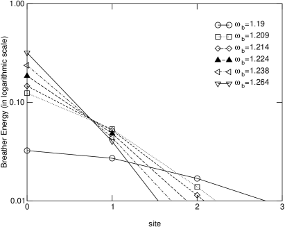
Figure 1: Local breather energy (in logarithmic scale) as a function of site number (central site at 0). We take as a reference the value $0.01$ in energy thus neglecting local energies below this value. For the three lower frequencies breather is localized in 5 sites and for the other three frequencies the breather is localized in 3 sites.

In order to construct the PIM with local spin $S_{i}$ we use the following projector:

$${\cal{P}}_{i}E_{i}=S_{i}$$ (2)

where $E_{i}$ is the local energy at site i. The value of the spin $S_{i}$ is then $S_{i}=+1$ for $E_{i}\geq E_{th}$ and $S_{i}=-1$ for $E_{i}<E_{th}$ . Thus, by construction, all positive spins correspond to breather states while negative spins to linear lattice modes. As the dynamical system evolves in time, so does the corresponding Ising model through dynamical spin flipping. Whenever there is spontaneous energy accumulation, there will be spin up tendency while when breathers are destroyed the spins will flip down. The overall spin configuration of PIM will determine the state of the system and microscopic dynamical events will determine the specific changes in the spin distribution. Even though there is no explicit Ising-like Hamiltonian for PIM, the local dynamics introduces effective spin-spin interactions that may be quite complex, competing as well as time dependent. As a result, we expect the thermodynamics to be quite rich with novel aspects.

3 The order parameter

The pseudospin Ising model that we established for the hard-$\phi^{4}$ lattice has no direct Hamiltonian representation like the standard Ising model. Nevertheless spin degrees of freedom change as a result of two factors, one is the contact to a bath that produces and destroys statistically breathers while the second is the local breather dynamics itself that can have similar effects. Although hard to separate the two, the latter tendency can be seen as a local fluctuating effective spin-spin interaction, similar in some sense to the competing interaction found in a spin glass (SG). We note that while in the latter at zero external field there is no net magnetization $m$ in our PIM the value of $m$ is typically nonzero by construction. Although the transition from negative to positive averaged magnetization marks the transition from a phonon-dominated to a breather-dominated system, the non-zero value of $m$ differentiates PIM from a usual SG model. Nevertheless the presence of breathers at finite temperatures is seen as a local persistence of the pseudospins in the PIM. This persistence introduces short range order in the model and affects directly higher correlation spin functions, such as susceptibility. The relevant quantity that probes these correlations is the Edwards-Anderson order parameter originally introduced for spin systems with competition[12, 13, 11]. In order to analyze its properties we will use two approaches, one is a replica representation based on ensembles and the second is an analysis in the time domain. Although in standard statistical mechanical systems ergodicity warranties the equivalence between phase space averages and time domain averages, this is not necessary true in more complex systems with some form of competition build in; the case treated here of the extended nonlinear systems belongs in the latter category.

3.1 Replica representation

In spin glasses the replica approach is used in order to compute the partition function of the system in the space of variables where the effective Hamiltonian does not contain any disorder and is translationally invariant [11]. Replicas not only help in writing down theoretical relations, but additionally the replica formalism is very powerful when many near equilibrium states of different free energy exist. Operationally, different replicas can be thought of as clones of the original system, viz. different statistical realizations of the same equilibrium system corresponding to different sets of initial conditions while the overlap between different replicas can be thought of as a measure of the similarity between them [14]. The reason for the applicability of replica ideas in the case of breathers is because the latter, being long-lived metastable states, induce state persistence in the nonlinear system and thus non-zero overlap between different system realizations. As has been already noted in several works, the time regime in which standard Gibbsian statistical mechanics is applicable is not very interesting in most cases.

In order to implement these ideas in the statistical enumeration of states and study of thermodynamic properties we introduce system replicas in the following way: We consider the Hamiltonian lattice of $N$ sites (typically $N=200$) and introduce initial conditions with random initial velocities following the Gaussian distribution at temperature $T$, i.e. we start with thermalized velocities but not thermalized positions. Clearly the system is out of equilibrium, but not too far from it. We then let the system evolve for a time $t_{1}$ that is approximately one hundred periods of the cutoff breather period related to the energy threshold; at the same time we employ numerically the projection operation and thus turn the nonlinear system into an effective spin system. Longer $t_{1}$-times such as $t_{1}$ approximately $270$ periods does not alter the results. While in the time window $t_{1}<t<t_{2}$ we average the spin values and the outcome defines one system replica. This procedure is repeated $n$ times for different initial conditions and the resulting ensemble constitutes the replica ensemble at temperature $T$. The typical numbers used are $n=100$ while $t_{1}=400$ and $t_{2}=500$ (approximately $78$ and $97$ periods of the cutoff breather period respectively); ensembles up to $n=200$, size of the lattice up to $N=1000$, longer times as well as no averaging in the selected time range were also tested with small changes in the results. We note that the averaging done in the time range $[t_{1},t_{2}]$ simply smooths somehow the spin distribution of each replica and produces changes only in cases when moving breathers are present. The replica ensemble thus generated can be thought off as the equivalent equilibrium ensemble for the nonlinear system. We can now use this ensemble in order to compute the averaged replica magnetization defined through

$$m=\frac{1}{\tau~{}n~{}N}\sum_{t=t_{1}}^{t_{1}+\tau}\sum_{\alpha=1}^{n}\sum_{i=1}^{N}S_{i}^{\alpha}(t)=\frac{1}{nN}\sum_{\alpha=1}^{n}\sum_{i=1}^{N}S_{i}^{\alpha}$$ (3)

where $\tau$ is the time window $\tau=t_{2}-t_{1}$ that is used for the replica construction and $S_{i}^{\alpha}$ is the time independent spin at lattice site $i$ belonging to replica $\alpha$. We note that even though the time $t_{1}$ is long enough for the system to reach local thermal equilibrium it is certainly not sufficiently long for the system to reach true thermodynamic equilibrium. This is clearly observed from the presence of persistent modes in the dynamical lattice or the induced short range order in the pseudospin model. The temperature $T$ of the system is defined through averaged equipartition and the system itself is now represented by the collection of the $n$ equivalent time independent replicas. The short range order induced by nonlinear localization introduces some similarity between the replicas, even though they were produced in a statistically independent fashion. This similarity between a random pair of replicas $\alpha$ and $\beta$ can be quantified though the introduction of the replica overlap:

$$q^{\alpha\beta}=\frac{1}{N}\sum_{i=1}^{N}S_{i}^{\alpha}S_{i}^{\beta}$$ (4)

The quantity $q^{\alpha\beta}$ evaluated for two specific replicas $\alpha$ and $\beta$ from the ensemble of $n$ replicas measures the degree of similarity between the two pseudospin configurations[11, 15]. Since $n$ is large and there are $n(n-1)/2$ overlaps one may define some additional quantities that help quantify the extent of replica similarity; one of those is the averaged overlap taken over all replica pairs and being equal to:

$$q=\frac{2}{n(n-1)}\sum_{\alpha,\beta=1,\alpha\neq\beta}^{n}q^{\alpha\beta}$$ (5)

Furthermore, the overlap distribution or probability density function $P(q^{\alpha\beta})$ that is easily evaluated may provide very detailed information for the system statistical modes. In the context of the Parisi theory[15], it can be used in order to evaluate the inverse overlap function $x(q)$ that is the cumulant distribution function of $P$, viz.

$$x(q)=\int_{-\infty}^{q}dqP(q)$$ (6)

According to the ideas believed to be true at least in the context of the mean field theory of spin glasses [13], the replica overlap $q(x)$ determined as the inverse function of $x(q)$ defined through Eq. (6), and evaluated at $x=1$, viz. $q(1)$ is identical to the maximum overlap $q_{max}$ between all pairs of the replica ensemble. Furthermore, this quantity $q_{max}$ is identified with the Edwards-Anderson order parameter for spin glasses that is able to probe into the short range order of these systems [15, 11]. In a regular system, the overlap distribution $P(q)$ is a delta function and, as a result, the maximum and averaged replica overlaps coincide. In a statistically inhomogeneous system on the other hand, the overlap distribution is more complex leading to mean overlap that is different from the maximal replica overlap. In these cases, the latter determines the tendency of system copies to be similar even though they were generated through a random procedure. The true thermodynamics of these systems is dictated by this property for replica similarity or proximity and as a result $q_{max}$ is a pivotal quantity.

We have performed the aforementioned analysis for the $n$ replicas of our system and evaluated both the average replica overlap $q$ as well as the averaged maximum overlap $q_{max}$ between the replicas. The outcome is shown in Fig.2 where $1-q$ and $1-q_{max}$ are plotted as a function of the averaged system temperature evaluated through equipartition. The specific functional choice for this representation is dictated by the fact that in a true magnetical system such as a spin glass, local spin susceptibility $\chi$ is related to the overlap $q$ for small fields as $k_{B}T\chi=1-q$ in spin glasses [11]. Thus, $1-q$ and $1-q_{max}$ are two measures of the pseudospin susceptibility evaluated through the averaged and maximal replica overlaps respectively. The factor $k_{B}T$ stems from local application of the fluctuation-dissipation theorem in standard spin systems; we will not include it in the pseudospin model although we will still refer to the two quantities derived through the replica overlaps as ”susceptibilities” and use the quantities $\chi$ and $\chi_{max}$ respectively to designate them. After these comments, we can now focus on the numerical results of Fig.2 and discuss the physics that is derived.

Figure 2: Susceptibilities $\chi=1-q$ (circles) and $\chi_{max}=1-q_{max}$ (diamonds) as a function of temperature (logarithmic scale in (a)). In (a) entire range while in (b) only in the vicinity of the transition point. We note the clear difference between $\chi$ and $\chi_{max}$ at high temperatures where discrete breathers are generated.

The general shape of the PIM susceptibility is similar to that of zero-field cooled spin glass susceptibility characterized by a reasonably sharp cusp at a characteristic temperature $T_{g}$ [11]. We call hereafter phase I the low temperature regime for $T<T_{g}$ while the high temperature regime for $T>T_{g}$ we call phase II. For $T\ll T_{g}$ both averaged and maximal overlaps give the same susceptibility while in the high temperature phase II for $T>T_{g}$ they are clearly different.

While for $T<T_{g}$ $\chi$ and $\chi_{max}$ raise to the maximum in a short temperature range, for $T>T_{g}$ they decay very slowly. At very low temperatures in phase I most dynamical states are phonon modes resulting in an ordered state of down spins leading thus to the greatest possible overlap at $T=0$, viz. $q=1$. As the temperature increases more and more breather modes are generated resulting in spin up states and a subsequent decrease of both the averaged and maximal overlaps. The reason for the reduction of the overlap is simple; since the breather modes are few and in random lattice locations, mixing different random realizations results in smaller overlap. When the temperature reaches the value $T_{g}\approx 0.38$ the average system magnetization becomes zero and a change in the thermodynamic behavior occurs. The onset of persistence due to the abundant breather modes results not only in a positive magnetization but also in persistence in the local pseudomagnetic features. This is demonstrated by two features of Phase II in Fig.2, one being the slow decay as a function of temperature of both susceptibilities while the other is the separation of the maximal from the averaged susceptibility. The slowness of this decay is contrasted to the fast rise on the low temperature size of phase I. The slow decay of $\chi$ in $T$ shows that in phase II the system establishes for each temperature local order that is not very sensitive to temperature changes, i.e. the system has some ”temperature rigidity”. This feature is compatible with the presence of a large number of breathers in the system and the fact that random initial conditions that do not differ very much result in similar system breather content. The second characteristic, viz. that of the different decay between $\chi$ and $\chi_{max}$ is a very significant one. It demonstrates that the overlap distribution $P(q)$ is not trivial and that in this regime replicas are now ”close” or similar, a feature that is clearly absent in the phase I. Physically this proximity of the random replicas in phase II is directly attributed to the persistence properties of the breather modes.

The contrast between the low and high temperature regime can be seen easily in an energy density plot and the resulting PIM representation in each case is shown in Figure (3). In Fig. 3(a) the system is at temperature $T=0.057$ ($k_{B}T<E_{g}$) while in (b) $T=0.533$ ($k_{B}T>E_{g}$). The horizontal axis labels the lattice sites, the vertical one is time while in darker regions the local oscillator energy is higher. In subfigures 3(a) and 3(b) we show the space-time evolution of the true local oscillator energy while in (c) and (d) we show what the system looks like after performing the pseudospin projection for each corresponding temperature and with black color labeling the spin up PIM states. In the first case (Fig. 3(a) and (c)) where breathers cannot occur due to low temperature of the system the mean magnetization is negative while in the second case (Fig. 3(b) and (d)) breathers have formed and the lattice has positive mean magnetization.

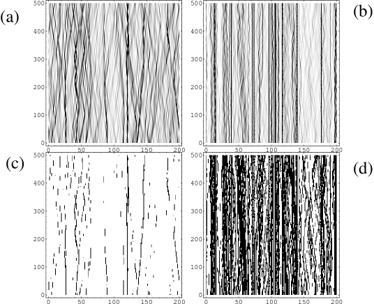
Figure 3: Energy density for a system with temperature (a) $T=0.057$ and (b) $T=0.533$ respectively; horizontal axis denotes lattice sites while the vertical axis denotes time. Black color indicates the more energetic regions. We note that the grey scales in (a) and (b) are normalized as intermediate colors between black and white and, as a result, correspond to different local energy content in each subfigure. Graphs (c) and (d) are the systems (a) and (b) correspondingly using the pseudospin representation. We now note a more precise concentration of high energy regions in each case. Black color designates spin up states.

Before closing the discussion on the pseudospin susceptibilities obtained through the replica method we should make two comments. Firstly, the value of the transition temperature $T_{g}$ clearly depends on the cutoff energy $E_{th}$ of the projector ${\cal{P}}_{i}$ although not in a trivial way. While different choices of the latter modify $T_{g}$, the changes in its precise value are not large. Furthermore even though the cutoff $E_{th}$ is determined heuristically, its physical meaning is very precise and thus model independent. We will add more insight into the issue of the physical basis of the cutoff below. Secondly, the function $\chi(T)$ is proportional to $m^{2}(T)$ for all temperatures, i.e. the replica overlap that determines $\chi$ is global and not local. This feature which is at variance with usual zero field spin glass behavior stems from the specific way of construction of the pseudospin model since the latter leads to non zero averaged magnetization for most temperatures. Thus, in some sense, PIM is related to a SG in the presence of an external field. We will comment further on this point in the conclusions.

3.2 Time domain statistical mechanics

In the previous section we investigated thermal PIM properties using a replica ensemble and found the existence of a high temperature phase with enhanced replica overlap. Let us now engage in a complementary, yet more computer intensive analysis, performed purely in the time domain and independent of the introduction of replicas. For this purpose we now introduce a time averaged local pseudospin correlation function as follows:

$$q_{i}(t)=\langle S_{i}(0)S_{i}(t)\rangle=\frac{1}{t_{obs}}\int_{0}^{t_{obs}}S_{i}(t^{\prime})S_{i}(t^{\prime}+t)dt^{\prime}$$ (7)

where the observation time $t_{obs}$ is taken to be much longer than the relatively short time scale $t_{1}$ or $t_{2}$ and typically equal to $t_{obs}=10^{4}$ in time units. This time-averaged correlation function is calculated numerically for large lattices of typical size $N=500$. The true dynamical correlation function is given by:

$${q\prime}=\lim_{t\to\infty}\lim_{N\to\infty}\frac{1}{N}\sum_{i=1}^{N}\langle S_{i}(0)S_{i}(t)\rangle=\lim_{t\to\infty}\lim_{N\to\infty}\bar{q}$$ (8)

where $\bar{q}=\sum_{i=1}^{N}\langle q_{i}(t)\rangle/N$ The quantity $q\prime$ measures spin-spin correlations that have not decayed at a given time $t$ when this time is taken to be infinite, i.e. very long compared to all characteristic times of the system. In the context of the Sompolinski theory for SG this quantity is shown to be identical to the Edwards-Anderson order parameter, viz. $q\prime=q_{EA}$[16]. In ordinary mean-field spin glasses at zero external field the non zero value of $q_{EA}$ marks the onset of short range order and the spin glass phase. One issue of importance is the order of performing the limits in Eq. (8). If we take first the time limit, then the system of finite size $N$ will have infinite time available to it and thus would traverse all the parts of phase space. Taking subsequently the thermodynamic limit would mean that time correlations will be equivalent to a Gibbs average. If, on the other hand, we take first the limit of $N\to\infty$ then the system can be trapped in some reduced region of phase space corresponding for instance in a given distribution of breather states and since its size is infinite it will not be able to escape from it even in infinite time. Clearly, in the latter case the correlation function is not a function of the whole accessible phase space but only of those long lived parts where the system gets trapped, i.e. the corresponding correlation function is not Gibbssian.

Figure 4: Susceptibilities $\chi=1-q$ (circles), maximal replica susceptibility $\chi_{max}=1-q_{max}$ (diamonds) and susceptibility $\chi\prime$ obtained from the dynamic overlap $q\prime$ ($\chi\prime=1-q\prime$, squares) as a function of temperature (in logarithmic scale in (a)). We note in (b) good coincidence between $\chi_{max}$ and $\chi\prime$ over the entire high temperature range where breathers are dominant.

The susceptibility $\chi\prime=1-q\prime$ of the correlation $q^{\prime}$ evaluated for times of the order $t\approx 10^{4}$ for system sizes $N=500$ is presented in Fig.4 as well as it is compared with the susceptibility $\chi_{max}$ determined in the previous section through the maximal replica overlap $q_{max}$. We observe that there is a good agreement between the two quantities, especially in the glassy higher temperature phase II although there are clear deviations in the transition region due to increase of fluctuations. This good numerical agreement, tested also for other parameter regimes, demonstrates that indeed it is the maximal replica overlap that corresponds to the long-time system correlation functions. In other words, the thermodynamics of phase II is dominated by averages over restricted minima in the system free energy. For, if we take into consideration all system copies corresponding to different sets of initial conditions we obtain the average magnetization or equivalently the overlap over all replicas that mixes uniformly all the states. The maximum replica overlap on the other hand selects only states in close proximity for each temperature and performs the averaging only over those states. We observe that the equality $q\prime=q_{max}\equiv q_{EA}$ that is expected theoretically in mean field spin glass theory holds also in our pseudospin dynamical lattice even though the regime identification in the two classes of systems is quite distinct. We comment between $\chi\prime$ and $\chi_{max}$ also that the deviations observed numerically in the transition region are very likely attributed to the numerical time limitations in the evaluation of $q\prime$.

We note that the equality between maximal replica overlap and time correlation function that was found previously does not hold in cases where the dynamical system is in a regime that does not generate breathers. We have constructed a PIM also in the case with a linear on-site potential setting the same energy threshold that, nevertheless, is highly artificial in this case. We found small differences between the replica averaged, maximum overlap and spin-spin correlation function in this case. More specifically, the replica averaged and the spin-spin correlation coincide and the maximum overlap has small differences from the other two quantities. In Fig.5 we show the results for the linear model in the higher temperature phase, as well as, for comparison, the corresponding values of the nonlinear model. We observe a sharp contrast in the scale of the agreement of the various quantities in the linear versus the nonlinear case. We note, however, that in the transition region the fluctuations are more pronounced, a fact that is expected.

Figure 5: Nonlinear case susceptibilities $\chi=1-q$ (circles), maximal replica susceptibility $\chi_{max}=1-q_{max}$ (diamonds) and susceptibility $\chi\prime$ obtained from the dynamic overlap $q\prime$ ($\chi\prime=1-q\prime$, squares) as in Fig. 4(b). Linear case susceptibilities $\chi=1-q$ (dotted circles), $\chi_{max}=1-q_{max}$ (triangles up), $\chi\prime$ (triangles left). Both sets of susceptibilities are plotted as a function of time in the high temperature regime. A sharp contrast is seen uppon comparing the three curves of the nonlinear lattice with those of the corresponding linear one.

We can make an analytical estimation of the transition temperature through the use of the following argument based on energy equipartition of a single oscillator. For a single harmonic oscillator with total energy $E$ and threshold energy $E_{th}$ the transition temperature can be found through the median of the Boltzmann distribution $exp(-\beta E)$ determined through the equation $\int_{E_{th}}^{\infty}e^{-\beta E}dE=\int_{0}^{E_{th}}e^{-\beta E}dE$. When this equation holds we have with equal probability a spin up or a spin down state and as a result the averaged magnetization is zero. The transition temperature is thus found to be:

$$k_{B}T_{c}=\frac{E_{th}}{ln2}.$$ (9)

The transition temperature for the linear lattice in the low coupling limit for energy cutoff $E_{th}=0.18$ is manifested trivially by Eq. (9) which gives $T_{c}=0.256$ and agrees quite well with the numerical result $T=0.26$. We handle numerically several different cutoff values and found that the value of $T_{c}$ is in a good agreement with the analytical predictions using Eq. (9). The nonlinear case is handled using the same argument i.e. the transition temperature is defined through $N_{+}=N_{-}$ where $N_{+}=\frac{1}{Z}\int_{E_{th}}^{\infty}e^{-\beta E}\frac{d\Gamma}{dE}dE$ and $N_{-}=\frac{1}{Z}\int_{0}^{E_{th}}e^{-\beta E}\frac{d\Gamma}{dE}dE$ and $\frac{d\Gamma}{dE}$ is the density of states. We found strong deviations between the result resulting from this one oscillator based calculation and the numerical simulations. For the energy cutoff $E_{th}=0.18$, which is the one we mainly use, the transition point is through numerical simulation at $T_{g}=0.38$ while the value of temperature through the previous argument is at $T=0.288$. This disagreement holds for several other different cutoff values as well. We conclude that the transition temperature depends on the energy cutoff $E_{th}$ but in the nonlinear lattice case it is clearly dominated by other factors, viz. the formation of breathers. Our general conclusion from all the above comments is that the equality of the time correlation function $q\prime$ to $q_{max}$ and both to the Edwards-Anderson order parameter demonstrates that some form of glassiness for the high temperature phase is induced by the nonlinearly self-localized breather states.

4 Entropy of the pseudospin glass state, replica construction and initial conditions

Using the pseudospin representation for the nonlinear system we can produce easily an estimate of the part of the system entropy that is related to the onset of localized modes. In each temperature the $N$ pseudospins in each replica $n$ are partitioned in $N_{+}$ positive and $N_{-}=N-N_{+}$ negative ones. The entropy per spin is thus ($k_{B}=1$) :

$$S=\ln{N\choose N_{+}}=N\ln N-N_{+}\ln N_{+}-N_{-}\ln N_{-}$$ (10)

By construction, at low temperatures, negative spins dominate and the entropy is very small; upon increasing temperature, the entropy augments and reaches a maximum in the temperature where positive and negative spins are equal in number where $S=N\ln 2\approx 0.698N$. This transition temperature is equal to the one found through the system magnetization and susceptibility, viz. $T_{g}$, since the latter occurs near the point of zero pseudospin magnetization. For $T>T_{g}$ the entropy decays slowly as a function of temperature with a rate that is distinctly slower than that in phase I; these features are seen in Fig.6 where the numerically obtained entropy per spin is plotted as a function of temperature. The entropy reduction at high temperatures is a typical feature of coupled two level systems in one dimension. In the present model it corresponds to the saturation of the spin up states. The form of its occurrence is however different from those in the standard cases, for, in the present case it does not happen symmetrically for the low and high temperature phase. The slow decay in phase II compared to the fast rize in phase I captures the onset of order in the former case in the form of longer lived localized states.

We also comment that the calculated entropy measures the breather entropy evaluated over the appropriate free energy minima in the pseudospin representation. All replicas for $T>T_{g}$ are dominated by nonlinear localized modes and thus the number of up spins does not have a very strong temperature dependence. As a result, the calculated entropy is obtained from appropriate localized segments of phase space and not the entire phase space.

Figure 6: Numerically evaluated entropy per particle as a function of temperature for PIM.

Let us now focus on the dependence of the results on initial conditions. The role of the latter is critical for the the replica construction since they enable the system preparation in appropriate phase space states. Clearly the replica ensemble has to be produced randomly, yet the weight of nontrivial locally correlated states must be nonzero. As a result, true equilibrium initial conditions are not appropriate since they would not necessarily produce enough nonlinearly localized states and result simply in Gibbs state counting. This feature of the initial conditions has been discussed in Ref. ([6]). For our replica preparation we used a Gaussian distribution over the initial velocities but not the positions of the particles. As a result the system initially is away from equilibrium, yet not too far from it. Other initial conditions that are truly nonequilibrium will produce a larger weight of the correlated modes in the replica ensemble and as a result change the specific values obtained for the susceptibilities [6].

We have also performed the previous analysis using the Langevin equation approach. More specifically, for each temperature $T$ we thermalized the system using local stochastic noise and dissipation and used this state as the initial one for the preparation of the replicas as in section III. We found the following departures compared to the results presented earlier. Firstly the transition temperature $T_{g}$ was shifted to a smaller value, i.e. the transition to the glass phase occurs earlier. Furthermore, the tail distribution for the averaged $\chi$ is not as slow as for the other initial conditions while there is now a smaller difference between $q$ and $q_{max}$. Also in the case of Langevin thermalization $q$ and spin-spin correlation function coincide together. These features corroborate the statements made previously regarding the use of thermalized initial conditions. Similar observations have been made in other studies where a comparison among different thermalization processes where adopted.

5 Conclusions

The analysis of thermal properties of extended nonlinear lattice systems in their weak coupling limit is a task of paramount importance and difficulty due to the formation of nonlinear localized modes. The latter act as system impurity modes that nevertheless are self-generated and somehow annealed in the system. They have considerable resilience to thermal fluctuations, yet they are produced and destroyed by them. Their presence modifies the free energy landscape of the system and thus the resulting thermodynamics, leading to some form of system glassiness. In order to tackle these issues we first modified our dynamical system and turned it into an effective spin system of Ising type where the two spin values where determined from the the system dynamics through a projection. Locations with nonlinear energy accumulation were mapped to spin up states while the rest to spin down states. This reduction of the dynamical system into a spin model enables the use of the extended literature of spin glasses where similar issues have been addressed.

In order to handle the presence of long-lived breather modes in the lattice we used two approaches, one based on system cloning into replicas while the other in time domain correlation function evaluation. The replicas where constructed from a random ensemble of initial velocities and subsequent system evolution to times that are long for reaching local equilibrium but not long enough for breather destruction. The replicas are introduced in order to probe into equilibrium thermodynamics while the system is trapped in very long-lived metastable states. The basic quantity of interest is the degree of replica overlap that is directly connected to system susceptibility. We found that the averaged replica overlap leads to a susceptibility that has a relatively sharp maximum at a given temperature $T_{g}$ while its values for $T>T_{g}$ decay slowly with temperature signifying the presence of a phase with short range order induced by the breather modes. The glassy feature of this phase is demonstrated by the clear difference between the averaged and the maximal replica overlaps obtained through the calculation of the overlap distribution. Use of a complementary approach in the time domain shows that the dynamical correlation function evaluated for large systems and long times coincides with the maximal replica correlation obtained from the replica distribution function. This specific property shows that the high temperature phase corresponds to an averaged state over specific sectors of the phase space related to the presence of nonlinear localized modes and not to the entire system phase space.

While a reduction of continuous variables into a binary spin variable might seem at first highly artificial, it is in tune however with the natural bimodality that the presence or absence of a breather at each system neighborhood introduces. As a result, the pseudospin model we introduced has virtues as well as weaknesses. It is simple enough to be handled with ease as well as to clarify the connection of nonlinear lattice physics with spin glass ideas. While in our case of interest there is no quenched disorder, this role is played by the spontaneous onset of nonlinear localization, viz. the breathers. The connection of the dynamical system to a spin system enabled us to identify a transition to a high temperature phase that has glassy properties. This feature is distinct from ordinary glasses since in the latter it is the lower temperature phase that is the glassy one while the phase at higher temperature is in liquid form. In our case however, the system at low temperatures is linear and thus ordered, leading to a normal state. Glassines in the higher temperature phase is obtained due to the spontaneous generation of localized modes and the accompanied short range order found in the spin system.

One feature of PIM that is not very satisfying is that the formation of the specific spin states at each site depends on the local projector with an energy threshold. While the concept of the threshold is physically clear, its value is determined heuristically yet it is physically motivated. Furthermore, its specific form produces an approximate spin representation that in the cases of single breathers with some extent underestimates the local coherence. While the projection enables the construction of a spin model and thus makes a contact with the spin glass theory, the PIM is not a standard spin model and contains some undesirable features, such as the build in non-zero magnetization. These model deficiencies do not affect however the true value of the model to initiate a quantitative study of the glassy breather phase with proper concepts and methods. In a subsequent study we will present the physics of this phase as well as the correlation dynamics in the transition region independently of the pseudospin model.

We acknowledge partial support from European Union under HPRN-CT-1999-00163 and HPMF-2002-01965 and the Institute of Plasma Physics of the University of Crete.

References

- [1] G. P. Tsironis and S. Aubry, Phys. Rev. Lett. 77, N 26, (1996) 5225, A.Bikaki, N. K. Voulgarakis, S. Aubry and G. P. Tsironis, Phys. Rev. E 59, N 1, (1999), 1234.
- [2] A. J. Sievers and S. Takeno, Phys. Rev. Lett. 61, 970 (1988).
- [3] R. S. Mackay and S. Aubry, Nonlinearity 7, 1623 (1994).
- [4] S. Aubry, Physica D 71, 196 (1994)
- [5] M. Peyrard, Physica D 119, 184, (1998)
- [6] K. O. Rasmussen, S. Aubry, A. R. Bishop and G. P. Tsironis, Eur. Jour. Phys. B 15, 169 (2000).
- [7] R. Roncaglia and G. P. Tsironis, Physica Scripta 61, 123 (2000).
- [8] M. Peyrard and J.Farago, Physica A 288, 199 (2000).
- [9] R. Reigada, A. H. Romero, A. Sarmiento and K. Lindenberg, J. Chem. Phys. 111, 1373 (1999).
- [10] F. Piazza, S. Lepri and R. Livi, Chaos 13, 637 (2003).
- [11] K. Binder and A. P. Young, Rev. Mod. Phys., 58, N 4, (1986), 801.
- [12] S. F. Edwards and P. W. Anderson, J. Phys. F5, 965 (1975).
- [13] D.Sherrington and S. Kirkpatrick, Phys. Rev. Lett. 35, N 26, (1975) 1792.
- [14] S. C. Manrubia and A. S. Mikhailov, Europhys. Lett. 53, (2001), 451.
- [15] G. Parisi, Phys. Rev. Lett. 50, N 24, (1983), 1946.
- [16] H. Sompolinsky, Phys. Rev. Lett. 47, N 13, (1981), 935.