Heuristic Segmentation of a Nonstationary Time Series

Abstract

Many phenomena, both natural and human-influenced, give rise to signals whose statistical properties change under time translation, i.e., are nonstationary. For some practical purposes, a nonstationary time series can be seen as a concatenation of stationary segments. However, the exact segmentation of a nonstationary time series is a hard computational problem which cannot be solved exactly by existing methods. For this reason, heuristic methods have been proposed. Using one such method, it has been reported that for several cases of interest—e.g., heart beat data and Internet traffic fluctuations—the distribution of durations of these stationary segments decays with a power law tail. A potential technical difficulty that has not been thoroughly investigated is that a nonstationary time series with a (scale-free) power law distribution of stationary segments is harder to segment than other nonstationary time series because of the wider range of possible segment sizes. Here, we investigate the validity of a heuristic segmentation algorithm recently proposed by Bernaola-Galván et al. [Phys. Rev. Lett. 87, 168105 (2001)] by systematically analyzing surrogate time series with different statistical properties. We find that if a given nonstationary time series has stationary periods whose size is distributed as a power law, the algorithm can split the time series into a set of stationary segments with the correct statistical properties. We also find that the estimated power law exponent of the distribution of stationary-segment sizes is affected by (i) the minimum segment size, and (ii) the ratio $R\equiv\sigma_{\epsilon}/\sigma_{\bar{x}}$ where $\sigma_{\bar{x}}$ is the standard deviation of the mean values of the segments, and $\sigma_{\epsilon}$ is the standard deviation of the fluctuations within a segment. Furthermore, we determine that the performance of the algorithm is generally not affected by uncorrelated noise spikes or by weak long-range temporal correlations of the fluctuations within segments.

I Introduction

A stationary time series has statistical properties that do not change under time translation Stratonovich81 . Interestingly, the time series that arise in a large number of phenomena in a broad range of areas—including physiologic systems, economic systems, vehicle traffic systems, and the Internet Ivanov ; Bunde00 ; Goldberger02 ; Stanley02 ; Musha76 ; Leland95 ; Paxson96 ; Crovella97 ; Takayasu ; Abbot99 —are nonstationary. Thus nonstationarity is a property common to both natural and human-influenced phenomena. For this reason, the statistical characterization of the nonstationarities in real-world time series is an important topic in many fields of research and numerous methods of characterizing nonstationary time series have been proposed Method .

One useful approach to quantifying a nonstationary time series is to view it as consisting of a number of time segments that are themselves stationary. The statistical properties of the segments (i) can help us better understand the overall nonstationarity of the time series and (ii) yield practical applications. For example, developing control algorithms for Internet traffic will be easier if we understand the statistical properties of these stationary segments—a behavior that directly corresponds to the “coarser flow rate” of the current network traffic.

In general, it is impossible to obtain the exact segmentation of a nonstationary time series because of the complexity of the calculation. An exact segmentation algorithm requires a computation time that scales as $O(N^{N})$, where $N$ is the number of points in the time series. Hence, such an algorithm is not practical. For this reason, the segmentation of a real-world time series must accomplish a trade-off between the complexity of the calculation and the desired precision of the result.

Bernaola-Galván and co-workers recently proposed a heuristic segmentation algorithm Segment designed to characterize the stationary durations of heart beat time series. In this algorithm Segment , the calculation cost is reduced by iteratively attempting to segment the time series into only two segments. A decision to cut the times series is made by evaluating a modified Student’s $t$-test for the data in the two segments.

The application of this segmentation algorithm reveals that the distribution of the stationary durations in heart beat time series decays as a power law Segment . Intriguingly, a recent analysis of Internet traffic uncovered that the distribution of stationary durations in the fluctuation of the traffic flow density also follows a power law dependence Fukuda01 . Because these signals have their origin in such diverse contexts, these findings suggest that the power law decay of the distribution of the stationary period may be a common occurrence for complex time series. Thus, the correct implementation and interpretation of the results obtained by the segmentation algorithm is essential in understanding the dynamics of the system. In fact, there are many implementation issues concerning the segmentation algorithm of Ref. Segment that have not yet been addressed explicitly in the literature, especially those concerning the proper estimation of the value of the power-law tail’s exponent in the cumulative distribution of stationary durations.

In this paper we systematically analyze different types of surrogate time series to determine the scope of validity of the segmentation algorithm of Bernaola-Galván and co-workers Segment . In Section II, we briefly explain the segmentation algorithm. In Section III, we present results for the dependence of the exponent of the power law tail on the minimum size of the segments in the distribution of the stationary durations. In Section IV, we consider the effect of the amplitude of the noise and the presence of spike-type noise. In Section V we consider long-ranged temporally-correlated noise. Finally, in Section VI, we summarize our findings.

II Implementing the Segmentation Algorithm

II.1 The algorithm

To divide a nonstationary time series into stationary segments Segment , we move a sliding pointer from left to right along the time series and, at each position of the pointer, compute the mean of the subset of the signal to the left of the pointer $\mu_{\rm left}$ and to the right $\mu_{\rm right}$. For two samples of Gaussian distributed random numbers, the statistical significance of the difference between the means of the two samples, $\mu_{1}$ and $\mu_{1}$, is given by the Student’s $t$-test statistic prob_intro

$$t\equiv\left|\frac{\mu_{1}-\mu_{2}}{S_{D}}\right|,$$ (1)

where

$$S_{D}=\left(\frac{(N_{1}-1)s_{1}^{2}+(N_{2}-1)s_{2}^{2}}{N_{1}+N_{2}-2}\right)^{1/2}\left(\frac{1}{N_{1}}+\frac{1}{N_{2}}\right)^{1/2}$$ (2)

is the pooled variance NRC , $s_{1}$, $s_{2}$ are the standard deviations of the two samples, and $N_{1}$ and $N_{2}$ are the number of points in the two samples.

Moving the pointer along our time series from left to right, we calculate $t$ as a function of the position in the time series. We use the statistic $t$ to quantify the difference between the means of the left-side and right-side time series. Larger $t$ means that the values of the mean of both time series are more likely to be significantly different, making point $t_{\rm max}$, with the largest value of $t$, a good candidate as a cut point.

We then calculate the statistical significance $P(t_{\rm max})$. Note that $P(t_{\rm max})$ is not the standard Student’s $t$-test because we are not comparing independent samples. $P(t_{\rm max})$ is numerically approximated as

$$P(t_{\rm max})\approx\{1-I_{[\nu/(\nu+t_{\rm max}^{2})]}\times(\delta\nu,\delta)\}^{\gamma},$$ (3)

where $\gamma=4.19\ln N-11.54$ and $\delta=0.40$ are obtained from Monte Carlo simulations Segment , $N$ is the size of the time series to be split, $\nu=N-2$, and $I_{x}(a,b)$ is the incomplete beta function.

If the difference in mean is not statistically significant—i.e., if is smaller than a threshold (typically set to 0.95)—then the time series is not cut. If the difference in means between the left and right part of the time series is statistically significant, then the time series is cut into two segments as long as the means of the two new segments are significantly different from the means of the adjacent segments. If the time series is cut, we continue iterating the above procedure recursively on each segment until the obtained significance value is smaller than the threshold, or the size of the obtained segments is smaller than a minimum size $\ell_{0}$. We will see that the value of $\ell_{0}$ is one of the parameters controlling the accuracy of the algorithm.

II.2 Surrogate Time Series

To investigate the validity of the algorithm, we analyze surrogate time series $x(t)$ generated by linking segments with different means. As described in Section I, the cumulative distribution of the stationary durations for some real-world time series is characterized by a power law decay in the tail, so the probability of finding a segment of size larger than $m$, i.e., the cumulative distribution of segment sizes in our time series, is

$$P(>m)=\frac{\gamma+1}{m_{0}^{\gamma+1}}m^{-\gamma},\ \ \ \mbox{for}\ m\gg m_{0},$$ (4)

where $m_{0}$ is the minimum size of a segment.

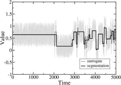
Figure 1: Surrogate time series constructed according to the procedure described in II.B with parameters $m_{0}=20$, $\gamma=1.0$, and $R=1$. The time series is drawn in light gray, and the stationary segments are represented by a dark gray line. The black line displays the output of the segmentation algorithm for $\ell_{0}=50$. It is visually apparent the black line provides a adequate coarse-grained description of the surrogate time series. Note also that the algorithm cannot extract the smallest segments because of the restrictions on resolution for $m<\ell_{0}$.

We generate time series with a power law distribution of segment sizes by the following procedure:

1. draw from the interval [$m_{0}$,+$\infty$] a sequence of segment lengths {$m_{i}$} with distribution given by Eq. (4);

2. draw from the interval [0,1] a sequence of mean time series values $\bar{x}_{i}$ with uniform probability;

3. draw from the interval [-$\sqrt{3}\sigma_{\epsilon}$,$\sqrt{3}\sigma_{\epsilon}$] a sequence of fluctuation values $\epsilon_{i}(k_{i})$, for $k_{i}=1,\cdots,m_{i}$, with uniform probability.

The resulting time series is given by

$$x(t)=\bar{x}_{i}+\epsilon_{i}(k_{i})\,,$$ (5)

where $i$ is such that

$$\sum_{j=0}^{i-1}m_{j}<t\leq\sum_{j=0}^{i}m_{j}\,,$$ (6)

and $k_{i}$ is such that

$$k_{i}=t-\sum_{j=0}^{i-1}m_{j}\,.$$ (7)

To quantify the level of the noise, we define the ratio

$$R\equiv{\sigma_{\epsilon}\over\sigma_{\bar{x}}},$$ (8)

where $\sigma_{\bar{x}}$ is the standard deviation of the mean of the segments and $\sigma_{\epsilon}$ is the standard deviation of the fluctuations within a segment. For $\bar{x}$ uniformly distributed in the interval [0,1], $\sigma_{\bar{x}}=0.3$.

For each set of parameters ($R$, $\gamma$, $m_{0}$) we generate ten time series, each with 50,000 data points. Note that knowing a priori the value of $m_{0}$ in a real-world time series is unlikely, but in order to test the algorithm in a consistent way, we consider in the following section $m_{0}\geq 20$ because that is the resolution limit for the algorithm (see also Appendix A).

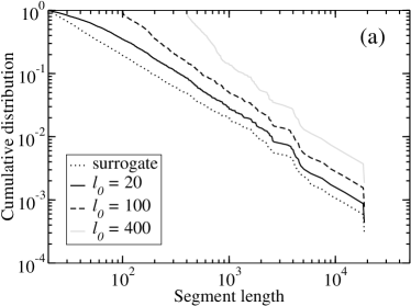
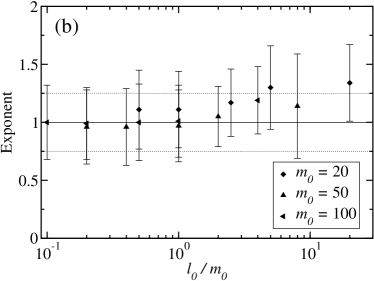
Figure 2: (a) Cumulative distribution $P(\ell)$ of segment sizes larger than $\ell$ for surrogate time series with 50,000 data points; $\gamma=1.0$, $R=1$ and $m_{0}=20$. The dotted line indicates the input segment size distribution for the surrogate time series. The slope of the line is $1.0$ for $20<m<\mbox{4,000}$. The other curves show $P(\ell)$ for different values of $\ell_{0}$. For $\ell_{0}=20$, the curve is well described in the range $100<\ell<\mbox{4,000}$ by a power law with $\hat{\gamma}\approx 1.0$. The distribution does not decay as a power law for $\ell<100$ due to the fact that the segmentation algorithm cannot split a time series with a number of points insufficient to perform the Student’s $t$-test. For $\ell_{0}=400$, $P(\ell)$ decays as a power law for $\mbox{1,000}<\ell<\mbox{8,000}$. The segmentation algorithm correctly splits all segments in the surrogate series with size $\ell>\mbox{1,000}$. (b) Dependence of $\hat{\gamma}$ on $\ell_{0}$ and $m_{0}$. The mean and the standard deviation of the exponent for the original time series is $1.05\pm 0.24$, shown by the black solid and dotted lines. The error bars show the standard deviation of the estimates $\hat{\gamma}$. For $\ell_{0}/m_{0}<5$, we find $\hat{\gamma}\approx 1$. Thus, the algorithm accurately estimates exponents in this region. However, the values of the exponent are close to 1.3 for $\ell_{0}/m_{0}>10$, meaning that $m_{0}\ll\ell_{0}$ leads to an overestimation of $\gamma$.

Figure 1 displays a surrogate time series, the corresponding stationary durations, and the result of the segmentation algorithm with $\ell_{0}=50$ and $m_{0}=20$. The segments obtained by the segmentation algorithm do not exactly match the stationary segments in the surrogate time series but the figure strongly suggests that the algorithm provides the correct coarse-grained description of the time series. As expected, the segmentation algorithm cannot extract segments with size $m<\ell_{0}$.

III Accuracy of the segmentation algorithm

III.1 Dependence on $\ell_{0}$ and $m_{0}$

Figure 2(a) displays the cumulative distribution of segment sizes, which is the probability of finding a segment with size larger than $\ell$ for a surrogate time series split for different values $\ell_{0}$. The cumulative distributions of the size of the stationary segments cut by the segmentation algorithm for surrogate time series are well fit by a power law decay. For all cases, we find

$$P_{\ell_{0},m_{0}}(>\ell)\sim\ell^{-\hat{\gamma}(\ell_{0},m_{0})}$$ (9)

with the same exponent value $\hat{\gamma}\approx 1.0$ GAMMA , indicating that the segmentation algorithm splits the nonstationary time series into segments with the correct asymptotic statistical properties. However, the range of scales for which we observe a power law decay with $\hat{\gamma}\approx\gamma$ depends strongly on the selection of $\ell_{0}$.

Table 1: Estimated exponent $\hat{\gamma}$, as defined by Eq. (5) for $\gamma=1.0$. The mean and the standard deviation of the exponents are calculated for the ranges indicated inside parenthesis using Eq. (11). The column labeled “input” presents exponent estimates obtained from the segment lengths used to generate the surrogate time series. We find $\hat{\gamma}\approx\gamma=1.0$ for $m_{0}<5\ \ell_{0}$.

	10	20	50	100	400	input
20	$1.1\pm 0.3$	$1.1\pm 0.3$	$1.2\pm 0.3$	$1.3\pm 0.4$	$1.3\pm 0.3$	$1.1\pm 0.3$
	($\ell>20$)	($\ell>20$)	($\ell>50$)	($\ell>110$)	($\ell>1000$)
50	$1.0\pm 0.3$	$1.0\pm 0.3$	$1.0\pm 0.3$	$1.1\pm 0.3$	$1.1\pm 0.5$	$1.0\pm 0.2$
	($\ell>50$)	($\ell>50$)	($\ell>100$)	($\ell>110$)	($\ell>1000$)
100	$1.0\pm 0.3$	$1.0\pm 0.3$	$1.0\pm 0.3$	$1.0\pm 0.3$	$1.2\pm 0.3$	$1.1\pm 0.3$
	($\ell>100$)	($\ell>100$)	($\ell>100$)	($\ell>100$)	($\ell>1000$)

For $\ell$ greater than about $5\ell_{0}$, the tails of the distributions are close to power law decays with $\hat{\gamma}\approx\gamma=1.0$. Moreover, all $P(\ell)$ follow the original curve for $\ell>\mbox{1,000}$, i.e., the algorithm correctly identifies the large segments independently of the selection of $\ell_{0}$. For $\ell<5\ell_{0}$, the distributions do not follow power law decays. The origin of this behavior lies in the fact that (i) for $\ell_{0}=20=O(m_{0})$, there are not enough data points to reliably perform the Student’s $t$-test, so one cannot reasonably expect any statistical procedure to be able to extract those short segments, and (ii) for $\ell_{0}\gg m_{0}$, one fails to extract many of the stationary segments. The reason for the latter is that the value of $\ell_{0}$ is in this case considerably larger than the size of the shortest segments in the time series, so the algorithm is forced to merge a number of short segments into longer ones with size greater than $\ell_{0}$. This process gives rise to an excess of segments with sizes between $\ell_{0}$ and $2\ell_{0}$.

Table 1 shows the mean and standard deviation of the estimated exponent value $\hat{\gamma}$ calculated from surrogate time series for several values of $m_{0}$ and $\ell_{0}$ (see Appendix A for details on how to to estimate $\hat{\gamma}$). Our results indicate that $\hat{\gamma}$ depends on both $m_{0}$ and $\ell_{0}$: If $\ell_{0}\gg m_{0}$, $\hat{\gamma}$ overestimates $\gamma$, while if $\ell_{0}\approx 0(m_{0})$, the algorithm correctly estimates the value of the exponent $\gamma$; cf. Fig. 2(b).

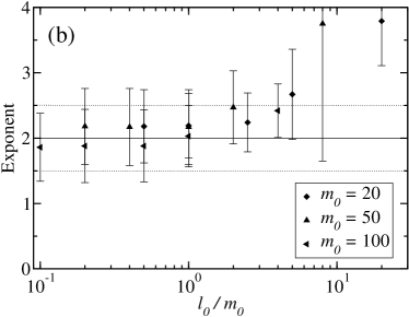
Figure 3: (a) Cumulative distribution of segment sizes for $\gamma=2.0$, $R=1$ and $m_{0}=20$. For $\ell_{0}=20$ and $100<\ell<\mbox{1,000}$, the exponent $\hat{\gamma}$ of the power law is close to $\gamma$. For $\ell_{0}=100$, we also $\hat{\gamma}\approx\gamma$. However, for $\ell_{0}=400$, the algorithm fails to split the time series correctly for $\ell<\mbox{1,000}$. Moreover, note that even though the exponent estimate is correct, the algorithm yields segments that are longer than the ones in the surrogate time series. (b) Dependence of $\hat{\gamma}$ on $\ell_{0}$ and $m_{0}$ for $\gamma=2.0$. For $\ell_{0}/m_{0}<4$, the algorithm yields segments with the correct statistical properties.

III.2 Dependence on $\gamma$

Next, we focus on the dependency of the accuracy of the segmentation algorithm on the value of $\gamma$. Figure 3(a) displays the cumulative distribution of segment sizes for surrogate time series generated with $\gamma=2.0$. A challenge for the segmentation algorithm is that Eq. (4) indicates that the probability of finding segments with size shorter than $4m_{0}$ is 90% for $\gamma=2.0$, which can lead to the “aggregation” of several consecutive segments of small size into a single longer segment.

As we found for $\gamma=1$, the tails of the distributions follow power law decays for large $\ell$, showing that the algorithm yields segments with the proper statistical properties. In Fig. 3(b), we show the dependence of $\hat{\gamma}$ on $\ell_{0}$ and $m_{0}$ for $\gamma=2.0$. We find that for $\ell_{0}/m_{0}<4$ the algorithm extracts segments with distributions of lengths that decay in the tail as power laws with exponents that are quite close to $2.0$ .

Table 2: Estimated exponents $\hat{\gamma}$ for $\gamma=2.0$. The mean and the standard deviation of the exponents are calculated for the ranges indicated inside parenthesis using Eq. (11). The column labeled “input” presents exponent estimates obtained from the segment lengths used to generate the surrogate time series. We find $\hat{\gamma}\approx\gamma=2.0$ for $m_{0}<4\ \ell_{0}$.

	10	20	50	100	400	input
20	$2.2\pm 0.6$	$2.2\pm 0.5$	$2.2\pm 0.5$	$2.4\pm 0.7$	$3.8\pm 0.7$	$2.2\pm 0.1$
	($\ell>100$)	($\ell>100$)	($\ell>100$)	($\ell>200$)	($\ell>800$)
50	$2.2\pm 0.6$	$2.2\pm 0.6$	$2.2\pm 0.6$	$2.5\pm 0.6$	$3.8\pm 2.1$	$2.1\pm 0.4$
	($\ell>100$)	($\ell>100$)	($\ell>100$)	($\ell>200$)	($\ell>1000$)
100	$1.9\pm 0.5$	$1.9\pm 0.6$	$1.9\pm 0.6$	$2.0\pm 0.5$	$2.4\pm 0.4$	$2.0\pm 0.4$
	($\ell>100$)	($\ell>100$)	($\ell>100$)	($\ell>200$)	($\ell>1000$)

Table 3: Estimated exponents $\hat{\gamma}$ for $\gamma=3.0$. The mean and the standard deviation of the exponents are calculated for the ranges indicated inside parenthesis using Eq. (11). The column labeled “input” presents exponent estimates obtained from the segment lengths used to generate the surrogate time series. For this value of $\gamma$, one finds that a small $m_{0}$ leads to a clear under-estimation of the $\gamma$. Note that the standard deviation of $\hat{\gamma}$ becomes larger, indicating the difficulty in obtaining $\hat{\gamma}$ accurately. Also noteworthy is the fact that because $\gamma$ is so large, the range of segment lengths $m$ drawn becomes much reduced. This implies that if one sets $\ell_{0}=400$ one is unable to properly estimate $\gamma$.

	10	20	50	100	400	input
20	$2.4\pm 0.5$	$2.3\pm 0.5$	$2.5\pm 0.5$	$2.7\pm 0.5$	$4.3\pm 1.4$	$3.1\pm 0.5$
	($\ell>100$)	($\ell>100$)	($\ell>100$)	($\ell>200$)	($\ell>1000$)
50	$3.0\pm 0.8$	$3.0\pm 0.8$	$3.0\pm 0.9$	$3.4\pm 0.6$	$5.9\pm 1.3$	$3.0\pm 0.6$
	($\ell>100$)	($\ell>100$)	($\ell>100$)	($\ell>200$)	($\ell>1000$)
100	$2.8\pm 0.9$	$2.8\pm 0.8$	$2.8\pm 0.9$	$2.8\pm 0.8$	$5.2\pm 1.7$	$2.9\pm 0.7$
	($\ell>200$)	($\ell>200$)	($\ell>200$)	($\ell>200$)	($\ell>1000$)

In Tables 2 and 3, we report the values of $\hat{\gamma}$ for $\gamma=2.0$ and $\gamma=3.0$, respectively. We find that for small $m_{0}$ and large $\gamma$, one over-estimates $\gamma$. Thus, we surmise that for $\gamma>3.0$, it becomes impractical to estimate $\gamma$ accurately, except for extremely long time series. This fact is not as serious a limitation as one may think because for large $\gamma$ it is always difficult to judge whether a distribution decays in the tail as an exponential or as a power law with a large exponent.

IV Robustness of the algorithm with regard to noise

IV.1 Amplitude of fluctuations around a segment’s mean

Another factor that may affect the performance of the segmentation algorithm of Bernaola-Galván and co-workers is the amplitude of the fluctuations within a segment. It is plausible that greater noise amplitudes will increase the difficulty in identifying the boundaries of neighboring segments. Thus, we next analyze the effect of the amplitude of the noise for surrogate time series.

Figure 4 demonstrates that for large R, the segmentation algorithm yields few short segments. This result arises from the concatenation of neighboring segments with means that become statistically indistinguishable due to the large value of $\sigma_{\epsilon}$.

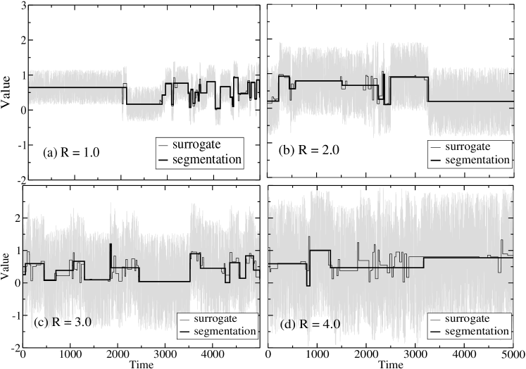
Figure 4: Surrogate time series for different amplitudes of the fluctuations within the segments. The surrogate time series were generated with $m_{0}=20$, $\ell_{0}=20$, $\gamma=1.0$, and (a) R = 1.0, (b) R = 2.0, (c) R = 3.0, and (d) R = 4.0. It is visually apparent that the segmentation algorithm yields longer segments as $R$ increases. This fact arises from the fact that the statistical test cannot distinguish two neighboring segments with close—relative to $\sigma_{\epsilon}$—means.

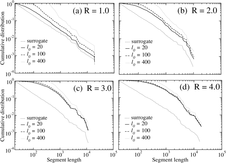
Figure 5: Cumulative distribution of segment size obtained with the segmentation algorithm for different amplitudes of the noise. As in Fig. 1, the time series analyzed were generated for $m_{0}=20$, $\gamma=1.0$, and (a) $R=1.0$, (b) $R=2.0$, (c) $R=3.0$, and (d) $R=4.0$. For $R\leq 3$, the tails of the distributions decay as power laws. For $R=4.0$, it is difficult to discriminate whether our the tails of distribution conform to exponential or power law decays. Note that as $R$ increases, the dependence of the functional form of the distributions on $\ell_{0}$ decreases appreciable.

We show in Fig. 5 the cumulative distributions of segment sizes for $\gamma=1.0$, $m_{0}=20$, and for different values of $R$. For large $\ell$ and $R\leq 3$, we find $\hat{\gamma}\approx\gamma$, while for $R=4$ the algorithm becomes ineffective at extracting the stationary segments in the time series. It is visually apparent that for $R=4.0$ the fluctuations within a segment are so much larger than the jumps between the means of the stationary segments that the segmentation becomes totally unable to parse the different segments; cf. Fig 4d.

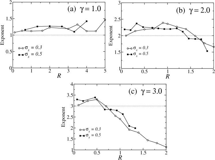
Figure 6: Dependence of $\hat{\gamma}$ on the ratio $R=\sigma_{\epsilon}/\sigma_{\bar{x}}$ for $m_{0}=20$, $\ell_{0}=20$ and three distinct values of $\gamma$: (a) $\gamma=1.0$, (b) $\gamma=2.0$, and (c) $\gamma=3.0$. The different curves in each plot correspond to different values of $\sigma_{\mu}$. For $\gamma=1.0$, we find $\hat{\gamma}=1.2$ for $0<R<4.0$, indicating that the algorithm is robust against increases in $R$. For $\gamma>1.0$, we find that the impact of an increasing $R$ on the performance of the algorithm becomes more and more marked. Specifically, for $\gamma=2.0$, we find $\hat{\gamma}\approx\gamma$ for $R<1.5$, while for $\gamma=3.0$, we find $\hat{\gamma}\approx\gamma$ for $R<0.6$.

In Fig. 6, we show $\hat{\gamma}$ for different values of $R$. For $\gamma=1.0$, we estimate $\hat{\gamma}\approx\gamma$ for $0<R<4$. In contrast, for $\gamma=2.0$, $\hat{\gamma}\approx\gamma$ only for $0<R<1.5$. When $R$ increases, the segmentation algorithm is unable to cut the segments because the greater amplitude of the fluctuations inside a segment decreases the significance of the differences between regions of the time series. This effect yields very large segments, which results in very small estimates of $\hat{\gamma}$. This effect is even stronger for $\gamma=3.0$, for which we find $\hat{\gamma}\approx\gamma$ only for $0<R<0.6$.

IV.2 Spike noise

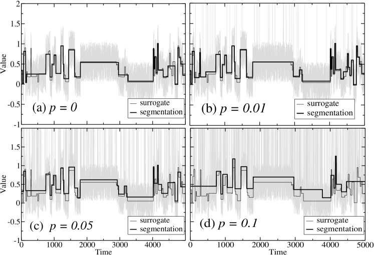
Figure 7: Surrogate time series with uncorrelated spike noise for $m_{0}=20$, $\gamma_{\epsilon}=0.3$, $\ell_{0}=20$, $\gamma=1.0$ and (a) $p=0$, (b) $p=0.01$, (c) $p=0.05$, and (d) $p=0.1$. For all values of $p$ considered, the application of the segmentation algorithm yields segments that, in a coarse-grained way, match well the segments in the surrogate data the.

Next we analyze the effect of spike noise on the performance of the segmentation algorithm. We generate surrogate time series as before and then for each $t$ make, with probability $p$, $x(t)=2$. The effect of this procedure is illustrated in Fig.7 for four distinct values of $p$. The figure also suggests that the segmentation algorithm yields a good coarse-grained description of the surrogate time series for $p$ as large as 0.1. This result suggests that the algorithm is robust to the existence of uncorrelated spike noise in the data (Fig. 8).

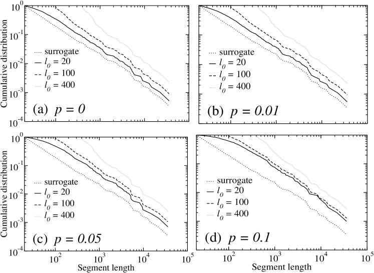
Figure 8: Cumulative distribution of segment sizes for surrogate time series with $\gamma=1.0$, $\sigma_{\epsilon}=0.3$, $m_{0}=20$, and for different densities $p$ of the spike noise: (a) $p=0.0$, (b) $p=0.01$, (c) $p=0.05$, and (d) $p=0.1$. The value of $x(t)$ is set at 2.0 for a spike. It is visually apparent that even for $p=0.1$ all the distributions decay as power laws for $\ell>200$ and that the slopes in the log-log plots are similar to the slope of the input distributions, i.e., the segmentation algorithm yields segments with the correct statistical properties even in the presence of strong spike noise.

V Correlated noise

In this Section, we investigate the effect of long-range correlations in the fluctuations around the segment’s mean on the performance of the segmentation algorithm. This study is particularly important because real-world time series often display long-range power law decaying correlations.

V.1 Segmentation of correlated noise with no segments

We generate a temporally-correlated noise whose power spectrum decays as $S(f)\sim f^{-\beta}$ Makse96 . The surrogate time series consists of 60,000 points, with mean 0. Figure 9 displays the cumulative distribution of segment lengths. The curves show the different noise correlations: $\beta=0.3$, 0.5, and 1.0 ($1/f$). Note that we have confirmed only one long segment for $\beta=0.0$, as one expects. On the other hand, for small $\beta$, we still observe a longer segment, although the curves decay rapidly for large $\beta$. Thus, the segmentation algorithm divides a correlated noise for large $\beta$ into many small pieces of stationary segments, because the given time series is already nonstationary for this case. Also, it is hard to determine the functional form of the plots for all cases. Even if the plots are assumed to follow power laws, the relationship between $\beta$ and $\hat{\gamma}$ is quantitatively obscure.

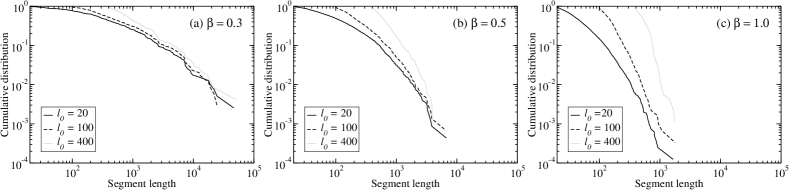
Figure 9: Segmentation of Guassian distributed long-range correlated noise with different exponent of the power law in the power spectrum density for the noise; (a) $\beta=0.3$, (b) $\beta=0.5$, and (c) $\beta=1.0$. We generate time series with 60,000 data points according to the modified Fourier filtering method (FFM) Makse96 . It is hard for all the curves to determine the functional form; a power law or an exponential distribution. There exists only one long segment for $\beta=0$. Then, for larger $\beta$, the segmentation algorithm splits the time series into many smaller pieces of stationary segments. This is because that the time series with larger $\beta$ has a higher probability that a part of the time series is nonstationary. However, a quantitative relationship between $\hat{\gamma}$ and $\beta$ is not clear for all the case of the correlated noise with no segments.

V.2 Segmentation of correlated noise with segments

Here, in order to show the ability of the identification of segments, we analyze surrogate time series concatenating segments with long-range correlated random variables whose power spectrum is followed by a power law with an exponent $\beta$. We show in Figs. 10(a)-(c) typical surrogate time series generated with $\gamma=1.0$, $m_{0}=20$, $R=1.0$, $\ell_{0}=20$, and different temporal correlations: (a) $\beta=0.1$, (b) $\beta=0.3$, and (c) $\beta=0.5$. The figure suggests that the segmentation algorithm can correctly parse the short segments but that long segments get cut multiple times, especially for $\beta=0.5$. This result is to be expected because the strong correlations in the noise lead to marked changes in the mean.

In Figs. 10(d)-(f), we show the cumulative distributions of segment sizes for $\beta=0.1,\ 0.3,\mbox{and }0.5$. The data confirm quantitatively the visual impression gained from Figs. 10(a)-(c), i.e., that longer segments get cut multiple times. In particular, for $\beta=0.5$, the distributions clearly deviate from the power law, independent of the selection of $\ell_{0}$. However, this fact should not be seen as a shortcoming of the algorithm; for large $\beta$, correlated noise for a long segment is already nonstationary, so that the algorithm is indeed cutting a nonstationary signal into stationary durations.

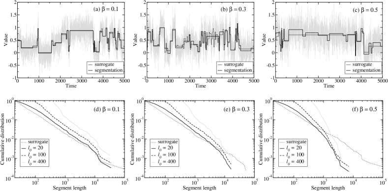
Figure 10: Surrogate time series with the long-range correlated noise and the result of the segmentation for (a) $\beta=0.1$, (b) $\beta=0.3$, and (c) $\beta=0.5$. The time series was concatenated by segments with the long-range correlated noise generated by the modified Fourier filtering method (FFM) Makse96 for $\gamma=1.0$, $m_{0}=20$, $\ell_{0}=20$, and $R=1$. For $\beta=0.1$ and $0.3$, the results of the segmentation algorithm resemble the segments in the surrogate time series. However, for $\beta=0.5$, it is visually apparent that long segment are cut multiple times, indicating that the algorithm judges the noise within a segment as a nonstationary time series. This is because that for large $\beta$, the correlated noise in a segment cannot be stationary. The same is not true for short segments, which are identified correctly under the above conditions. Cumulative distributions of the segument size for (d) $\beta=0.1$, (e) $\beta=0.3$, and (f) $\beta=0.5$. The distributions confirm the visual impression obtained form (a)-(c). In summary, the distributions decay faster than a power law when $\beta>0.3$, although they still follow a power law dependence for smaller $\beta$.

VI Discussion

In this paper we analyzed nonstationary surrogate time series with different statistical properties in order to investigate the validity of the segmentation algorithm of Bernaola-Galván and co-workers Segment . Our results demonstrate that this heuristic segmentation algorithm can be extremely effective in determining the stationary regions in a time series provided that a few conditions are fulfilled: First, one must have enough data points in the time series to yield a large number of segment lengths, otherwise one will not be able to reach the aymptotic regime of the tail of the distribution of segment sizes.

Second, the ratio of the amplitude of the fluctuations within a segment to the typical jump between the means of the stationary segments must be relatively small (less than about $0.6$) in order for one to trust the output of the segmentation algorithm. This concern contrast with the case of spike noise in the data which affects the performance of the segmentation algorithm only weakly.

Finally, if there are long-range temporal correlations of the fluctuations around the mean of the segment, then the segmentation algorithm correctly cuts the time series into the stationary segments for small $\beta$. However, for $\beta>0.3$, the fluctuations inside long segments become nonstationary, which results in the algorithm detecting many “stationary” durations inside these long segments.

Our analysis provides a number of clear guidelines for using effectively the segmentation algorithm of Bernaola-Galván et al. Segment :

1. One must perform the segmentation for a number of different values of $\ell_{0}$ in order to identify the region for which the tails of the distributions of segment sizes reach the asymptotic scaling behavior. (Note: If $\hat{\gamma}$ is large, than the estimation error can be quite considerable, especially if $m_{0}$ is small.)

2. One must calculate the ratio between the standard deviation of the mean value of the segment and the standard deviation of the fluctuations within a segment after performing the segmentation. If the $R$ than 0.6, then there is the possibility that $\hat{\gamma}$ is considerably under-estimating the true value of $\gamma$.

Acknowledgments

We thank S. Havlin, P. Ch. Ivanov, and especially P. Bernaola-Galván for discussions. We thank NIH/NCRR (P41 RR13622) and NSF for support. L.A.N.A. acknowledges a Searle Leadership Fund Award for support.

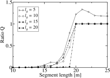
Figure 11: Algorithm’s resolution with regard to $\ell_{0}$ and $m$. We generate surrogate time series are constructed by the alternated concatenation of two types segments with fixed size $m_{0}$: one with mean 0.0 and standard dewviation 0.29 and another with mean 1.0 and standard deviations 0.29. We plot $Q$, which is defined in Eq. (10), as a function of $m$ for different values of $\ell_{0}$. Our results indicate that the segmentation algorithm is not able to extract the stationary segments for $m<20$ or $\ell_{0}<10$. Note also that $\ell_{0}\leq m$ for correct segmentation to occur.

Appendix A Performance of the algorithm for fixed segment sizes

As a special case, we analyze the time series whose stationary duration is fixed in order to discuss the minimum resolution of the segment algorithm. We concatenate segments with constant lenght $m$ with alternating means of 0.0 and 1.0. We then add fluctuations to those segments with a standard deviation of 0.29. We define the fraction of successfully split segments

$$Q\equiv\frac{\mbox{Number of segments correctly identified by the algorithm}}{\mbox{Number of segments in surrogate data}}\,,$$ (10)

where $Q=1.0$ corresponds to perfect segmentmentation.

We plot in Fig. 11 $Q$ as a function of $m$ for different values of $\ell_{0}$ . For $m<20$, the segmentation algorithm does not yield the correct segments in the surrogate time series even though the segment’s means are quite different. This result suggests that the resolution of the segmentation algorithm is $\approx 20$. We also find that for $\ell_{0}=5$, the algorithm splits the time series into too many segments. This result suggests that for optimal performance $\ell_{0}\geq 10$.

Appendix B Estimation of $\hat{\gamma}$

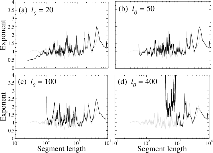
Figure 12: The behavior of the exponents $\hat{\gamma}(\ell_{n})$ of the power law in segment size distribution for different $\ell_{0}$; (a) $\ell_{0}=20$, (b) $\ell_{0}=50$, (c) $\ell_{0}=100$, and (d) $\ell_{0}=400$. $m_{0}=20$, $\gamma=1.0$. The exponent of the power law is calculated by Eq. (11), and plotted by black lines in the figure. The dotted gray lines also indicate the exponent of the surrogate time series for comparison. For $\ell_{0}=20$, the observed curve resembles the original one for $\ell>100$ and stays around 1.0, though the curve indicates an exponential decay for $\ell<100$. For $\ell_{0}=100$ and $400$, the segmentation results can follow the original ones for larger $\ell$; however, the estimated values of the exponent are somewhat overestimated for smaller $\ell$

To estimate the exponent $\hat{\gamma}$ of the power laws, we calculate the power law exponent at a segment size $\ell_{n}$ from a small region around $\ell_{n}$

$$\hat{\gamma}(\ell_{n})=\frac{\log(P(\ell_{n+\tau}))-\log(P(\ell_{n}))}{\log(\ell_{n+\tau})-\log(\ell_{n})},$$ (11)

where we set the region to $\tau=5$. Figure 12 shows the behavior of the power law exponent over $\ell$ corresponding to Fig. 2(a); the black lines are the behavior of the exponent at segment size $\ell$, and the broken lines are the behavior of the exponent of the power law in the distribution of the surrogate time series for comparison.

The range of $\ell_{n}$ for the calculation is between a starting point (where the exponential decay disappears) and 10,000. For $\ell_{0}=20$, the value of the exponent decreases for $\ell<100$, which corresponds to the exponential decay as shown in Fig. 2(a). However, the value of the exponent fluctuates around 1.0 for $\ell>100$, indicating that the algorithm can reproduce the correct statistical behavior. For $\ell_{0}=50$, the value of the exponent is close to 1.0 for $50<\ell<\mbox{10,000}$. Moreover, for $\ell_{0}=100$ and $400$, the curves decay quickly for the smaller $\ell$, and the value of the exponent tends to be overestimated.

References

- (1) R. L. Stratonovich, Topics in the Theory of Random Noise, Vol. 1 (Gordon and Breach, New York, 1981).
- (2) P. Ch. Ivanov et al., Nature 383, 323 (1996); P. Ch. Ivanov et al., Nature 391, 461 (1999);
- (3) A. Bunde et al., Phys. Rev. Lett. 85, 3736 (2000).
- (4) A. L. Goldberger et al., Proc. Nat. Acad. Sci. USA 99 Supp. 1, 2466 (2002).
- (5) H. E. Stanley, et al., Proc. Nat. Acad. Sci. USA 99 Supp. 1, 2561 (2002).
- (6) T. Musha and H. Higuchi, Jour. Appl. Phys. 15, 1271 (1976).
- (7) W. Leland et al., Trans. Net. 2, 1 (1995).
- (8) V. Paxson and S. Floyd, Trans. Net. 3, 226 (1996).
- (9) M. Crovella et al., Trans. Net. 5, 835 (1997).
- (10) M. Takayasu et al., Physica A 233, 924 (1996); M. Takayasu et al., Physica A 277, 248 (2001).
- (11) D. Abbott and L. B. Kish (eds), Unsolved Problems of Noise (Melville, New York, 1999).
- (12) C-K. Peng, et al., Chaos 5, 82 (1995); Z. R. Struzik, Fractals 8, 163 (2000).
- (13) P. Bernaola-Galván et al., Phys. Rev. Lett. 87, 16 (2001).
- (14) K. Fukuda et al., in preparation.
- (15) W. Feller, An Introduction to Probability Theory and Its Application, 2nd Ed., vol.1 (Willey, New York, 1971).
- (16) W. H. Press et al., Numerical Recipes in C (Cambridge University Press, Cambridge, 1988).
- (17) We use the notation as the abbreviation form of when the context is clear. Also, we use instead of .
- (18) H. A. Makse et al., Phys. Rev. E 53, 5445 (1996).