Dynamical model and nonextensive statistical mechanics of a market index on large time windows

Abstract

The shape and tails of partial distribution functions (PDF) for a financial signal, i.e. the S&P500 and the turbulent nature of the markets are linked through a model encompassing Tsallis nonextensive statistics and leading to evolution equations of the Langevin and Fokker-Planck type. A model originally proposed to describe the intermittent behavior of turbulent flows describes the behavior of normalized log-returns for such a financial market index, for small and large time windows, both for small and large log-returns. These turbulent market volatility (of normalized log-returns) distributions can be sufficiently well fitted with a $\chi^{2}$-distribution. The transition between the small time scale model of nonextensive, intermittent process and the large scale Gaussian extensive homogeneous fluctuation picture is found to be at $ca.$ a 200 day time lag. The intermittency exponent ($\kappa$) in the framework of the Kolmogorov log-normal model is found to be related to the scaling exponent of the PDF moments, -thereby giving weight to the model. The large value of $\kappa$ points to a large number of cascades in the turbulent process. The first Kramers-Moyal coefficient in the Fokker-Planck equation is almost equal to zero, indicating ”no restoring force”. A comparison is made between normalized log-returns and mere price increments.

Keywords: Econophysics; Returns; Tsallis nonextensive statistical mechanics; Fokker-Planck equation; detrended fluctuation analysis; power spectrum; Market dynamics; S&P500

PACS : 05.45.Tp, 05.10.Gg, 89.65.Gh

1 Introduction

The time lag dependent price increments, returns, log-returns, normalized log-returns of financial market indices, stocks and foreign currency exchange markets are known to be non-gaussian distributions and rather exhibit fat-tailed power-law distributions [1, 2, 3, 4, 5]. The origin of the so called large volatility characterized by such fat tailed distributions is a key question; the fat tails in such data are thought to be caused by some ”dynamical process” through a hierarchical cascade of short and long-range volatility correlations, though Gopikrishnan et al. consider that correlations and tails have different origins [5]. Destroying all correlations, e.g. by shuffling the order of the fluctuations, is known to cause the fat tails almost to vanish. It is still an open question whether both the fat-tailed power-law of partial distribution functions (PDF) of the various volatilities and their $evolution$ for different time delays in financial markets can be described.

The fat tails indicate an unexpected high probability of large price changes. These extreme events are of utmost importance for risk analysis. They are considered to be a set of strong bursts in the energy dissipation of so called clusters of high price volatility. In so doing the PDF and the fat tail event existence are thought to be similar to the notion of intermittency in turbulent flows [6]. Indeed employing the Fokker-Planck equation approach [7] recent studies [8, 9, 10, 11] have shown that the dynamics of a market results from a flow of information between long and short time scales. Since the distributions of returns obey a Fokker-Planck equation, the time evolution of the price $increment$ signal ($\Delta y$) measured for a time lag $\Delta t$ is governed by a Langevin equation [7]

$$\frac{d\Delta y}{d\Delta t}=D^{(1)}(\Delta y(\Delta t),\Delta t)+\eta(\Delta t)\sqrt{{D^{(2)}(\Delta y(\Delta t),\Delta t)}},$$ (1)

the drift $D^{(1)}$ and diffusion $D^{(2)}$ coefficients being those of the Fokker-Planck equation [8, 9, 10, 11]. It is often assumed that $\eta(\Delta t)$ is a correlated noise with gaussian statistics. Thus such a dynamics may be analogous to the dissipation of energy from large to small spatial scales in three dimensional turbulence as pointed out already in [6, 12, 13].

On the other hand, the non-Gaussian character of the fully developed turbulence [14] has been linked to nonextensive statistical physics [15, 16, 17, 18, 19, 20, 21, 22, 23]. Whence recently there has been a large number of studies, e.g. [6, 17, 24, 25, 26, 27] of financial markets employing the nonextensive statistics including those involving fully developed turbulence approach as in [14]. The nonextensivity, i.e. some anomalous scaling of classically extensive properties like the entropy, is linked to a single parameter $q$, e.g. in the Tsallis formulation of nonextensive thermostatistics.

In this paper on the study of the behavior of a financial index, i.e. the S&P500, on $large$ time windows, we apply as in [24, 27] for $short$ time windows, a recently suggested model of hydrodynamic turbulence that serves as a dynamic foundation for nonextensive statistics [19, 20, 21]. Indeed long time lag effects must be also investigated. Furthermore, it is known that some distinction must be made concerning the type of financial market $signal$ which is examined. We will compare results based on price increment and normalized log-return time series.

In Sect. 2, we describe the distribution of returns for the daily closing price signal of the S&P500 index for the time interval between Jan. 01, 1980 and Dec. 31, 1999, thus a series of $N=$5056 data points. Daily closing price values of the S&P500 index for the period of interest were downloaded from Yahoo web site . We characterize the tail(s) of the distribution for various $\Delta t$’s, i.e. from 1 up to 40 days, and will observe the value of the PDF tails, for such time lags, outside the best gaussian through the data. In Sect. 3, we calculate the power law exponents characterizing the $integrated$ distribution of the (normalized log-) returns over different time lags for the S&P500 index daily closing price through a detrended fluctuation analysis and a power spectral density analysis point of view. Results are compared to shuffled data for estimating the value of the error bars. In Sect. 4, Tsallis statistical approach is outlined, and distributions of (normalized log-) returns for time lags between $\Delta t$ = 1 to 40 days are examined. It is found that the $q$-value of the nonextensive entropy converges to a value = 1.22 for $\Delta t$ = 40 days, starting with $q$ = 1.39 for $\Delta t$ = 1, values similar to those reported for the intraday evolution of other financial indices, e.g. NASDAQ in [28] and slightly lower than those for S&P500 minute data [24]. The probability density $f_{\Delta t}(\beta)$ of the volatility $\beta$ in terms of the standard deviation of the normalized log returns of the S&P500 for different time lags is found to obey the $\chi^{2}$-distribution. The intermittency exponent ($\kappa$) of the Kolmogorov log-normal model is found to be related to the scaling exponent of the PDF moments, -thereby giving weight to the model. The large value of $\kappa$ points to a large number of cascades in the underlying turbulent process.

In Sect. 5, the usual Fokker-Planck approach for treating the time-dependent probability distribution functions is summarized and coefficients governing both the Fokker-Planck equation for the distribution function of normalized log returns and the Langevin equation for the time evolution of normalized log returns of daily closing price signal of S&P500 are obtained. We will notice that there is ”no restoring force”.

Therefore we present for the first time a coherent theory linking the shape and tails of partial distribution functions for long and short time lags of the daily closing values of a financial signal and connect the often suggested turbulent nature of the markets to a model encompassing nonextensive statistics and evolution equations of the Langevin and Fokker-Planck type. We are aware that the number of data points of the time series ($N=$5056) might seem quite small with respect to other studies involving millions of data points. Some previous work had indicated the possible use of 5000 or so data point series in order to obtain scaling arguments and ingredients for models [29, 30]. Clearly the relative error bars or confidence interval being roughly proportional to $N^{1/2}$ have to be taken with caution. Thus the conclusions universal value might be debated upon. Nevertheless one positive aspect might be that scaling effects are not too sensitive to $N$. We do warn however throughout the report that some caution might also be taken concerning the stationarity of the data. These $caveat$ might only be resolved through further work.

2 Distribution of returns

There are several ways of calculating the returns in a financial market. A simple one represents price increment $\Delta y(t,\Delta t)$ or difference between the value of the price signal $y(t)$ at time $t+\Delta t$ and its value at time $t$. Log-returns, i.e. the logarithm of the price ratio $\tilde{y}(t)=ln[y(t+\Delta t)/y(t)]$ are also used sometimes. Below we consider the normalized log-returns $Z(t,\Delta t)=(\tilde{y}(t)-<\tilde{y}>_{\Delta t})/\sigma_{\Delta t}$, where $<\tilde{y}>_{\Delta t}$ denotes the average and $\sigma_{\Delta t}$ the standard deviation of $\tilde{y}(t)$ for a given $\Delta t$. The normalized log-returns $Z(t,\Delta t)$ depend on the time $t$ and the time lag $\Delta t$. However, in order to simplify the notations and whenever possible without leading to confusion and misunderstanding we will drop the explicit writing of one or both variables. Daily closing price values of the S&P500 index for the period between Jan. 01, 1980 and Dec. 31, 1999 will serve as a standard financial signal $y(t)$, thus $N=$5056 data points.

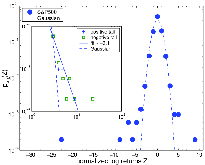
Figure 1: Probability distribution function of normalized log returns $Z(t,\Delta t)$ of daily closing price value signal of S&P500 between Jan. 01, 1980 and Dec. 31, 1999, for $\Delta t=1$ day (symbols). Normalized log returns are calculated as $Z(t,\Delta t)=(\tilde{y}(t)-<\tilde{y}>_{\Delta t})/\sigma_{\Delta t}$, where $\tilde{y}(t)=ln(y(t+\Delta t)/y(t))$ and $\sigma_{\Delta t}$ is the standard deviation of $\tilde{y}(t)$ for time lag $\Delta t$. The dashed line represents a Gaussian distribution. Inset: Power law fit (solid line) of the negative (-3.1) and positive (-3.1) slope of the distribution outside the Gaussian regime

The distribution of the normalized log-returns $Z(t,\Delta t)$ of the daily closing price signal for S&P500 index for the period between Jan. 01, 1980 and Dec. 31, 1999, for $\Delta t$ = 1 day are plotted in Fig. 1. A fit is first attempted with a Gaussian distribution for $small$ values of the increments, i.e. the central part of the distribution. This central part distribution is well fitted with such a Gaussian type curve within the interval $Z\in[-3,3]$ but departs from the Gaussian form outside this interval. The negative and positive tails of the distribution outside the Gaussian curve are found both to be equal to -3.1. In the case $\Delta t\geq$ 1 day, it is observed that the best Gaussian range is the same as for $\Delta t=1$ day (Fig. 2) but the outside tail values, as estimated for the various $\Delta t$’s of interest, are slightly different, and found to decrease with $\Delta t$; they are reported in Table 1. These findings ($\Delta t$-independent Gaussian range and tail exponent behavior) are at odd with the expectation that the PDF tends toward a Gaussian for large $\Delta t$. Some Bayesian-like analysis of the PDF’s, i.e. allowing for the expected Gaussian width behavior, has been done, with the appropriate conclusion. However, the error bar on the various widths do not allow for a statistically convincing evidence through the comparison of variance classical test. Same for the tail exponents which are obtained from a very small number of data points. Therefore it seems appropriate to pursue further the PDF analysis through other techniques that one allowing to extract a PDF tail from the difference between a raw data histogram and a central region Gaussian fit.

Notice that the Oct 19, 1987 and Oct. 27, 1997 crashes, as studied elsewhere [31, 32] are represented by isolated dots at $Z=-23$ and and $Z=-7$ respectively. The value of $Z=-8.7$ represents the aftershock crash of the Oct. 26, 1987 [32]. The analysis presented in the present study is not designed to capture such extreme events nor their effects.

3 Time correlations

There are different estimators for the long and/or short range dependence of fluctuations correlations [33]. In all cases it is useful to test the null hypothesis debated [4, 5] whether the fat tails are related to or/and caused by long-range volatility correlations. Destroying all correlations by shuffling the order of the fluctuations, is known to cause the fat tails almost to vanish. A Kolmogorov-Smirnov test (not shown) on shuffled data has indicated us the statistical validity of the numerical values and the statistically acceptable meaning of the displayed error bars.

Through the (linearly) detrended fluctuation analysis (DFA) method, see e.g. [34], we show first that the long range correlations of daily closing price signal of S&P500 for the time interval of interest, are brownian-like. The method has been used previously to identify whether long range correlations exist in non-stationary signals, in many research fields such as e.g. finance [29, 30], bioinformatics [35], cardiac dynamics [36] and meteorology [37, 38, 39]. The DFA concepts are therefore not repeated here. For an extensive list of references see [34]. Briefly, the signal time series $y(t)$ is $first$ $integrated$, to ”mimic” a random walk $Y(t)$. The time axis is next divided into $k+1$ non-overlapping boxes of equal size size $n$; one looks thereafter for the best (linear) trend, $z(n)$, in each box, and calculates the root mean square deviation of the (integrated) signal with respect to $z(n)$ in each box. The average of such values is taken at fixed box size $n$ in order to obtain

$$F(n)=\sqrt{\left<{1\over n}{\sum_{i=kn+1}^{(k+1)n}{\left[Y(i)-z(i)\right]}^{2}}\right>}.$$ (2)

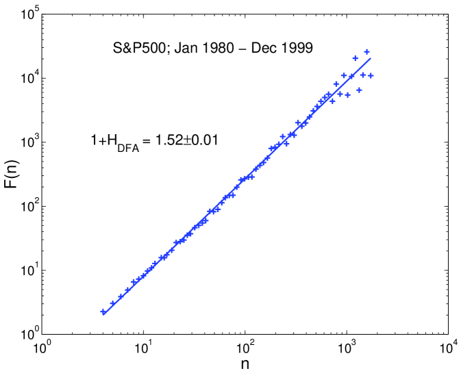
Figure 3: DFA function $F(n)$ plotted as a function of the the box size $n$ of the integrated daily closing price value signal of S&P500 between Jan. 01, 1980 and Dec. 31, 1999. Brownian-like fluctuations with $1+H_{DFA}=1.52\pm 0.01$ are obtained for all possible time scales

The box size is next varied over the $n$ value. The resulting function is expected to behave like $n^{1+H_{DFA}}$ indicating a scaling law characterized by a (Hurst) exponent $H_{DFA}$. For the (integrated) daily closing price signal of the S&P500 index, a scaling exponent $1+H_{DFA}=1.52\pm 0.01$ is found (Fig. 3) in a scaling range extending from about 1 week to about 250 days, i.e. 1 year.

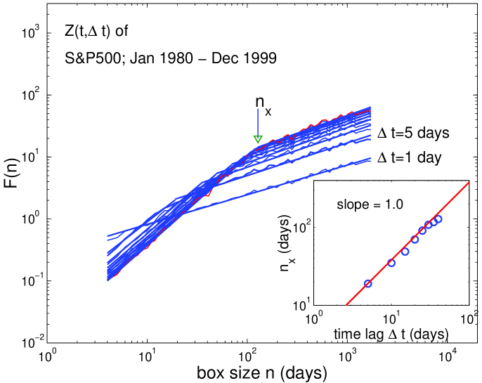
Figure 4: DFA function $F(n)$ plotted as a function of the the box size $n$ of the integrated normalized log returns $Z(t,\Delta t)$ of daily closing price value signal of S&P500 between Jan. 01, 1980 and Dec. 31, 1999 for different time lags $\Delta t=1,5,10,15,20,25,30,35,40$ days. Values of the scaling exponents $H_{DFA}$ for the various DFA functions are summarized in Table 2. Inset: Power law functional dependence of the value of the cross over box-size $n_{x}$ as a function of time lag $\Delta t$

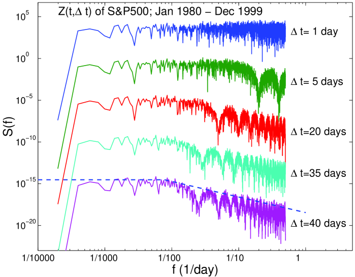
Figure 6: Power spectrum $S(f)$ of the normalized log returns $Z(t,\Delta t)$ of daily closing price value signal of S&P500 between Jan. 01, 1980 and Dec. 31, 1999 for different time lags $\Delta t=1,5,20,35,40$ days. Each curve is displaced by $10^{-5}$ with respect to the previous one; the power spectrum of the normalized log returns for $\Delta t=1$ day is not displaced. The dashed line from $f=1/70$ days^-1 to $f=1/2$ days^-1 has a slope $\mu=1.86$, corresponding to the $H_{DFA}$ exponent. The horizontal dashed line from $f=1/10^{-4}$ days^-1 to $f=1/128$ days^-1 corresponds to what should be expected for white noise and is in agreement with the scaling of the DFA function for the same data in Fig. 4

Along the same line of thoughts the scaling properties of the normalized log-returns $Z(t,\Delta t)=(\tilde{y}(t)-<\tilde{y}>_{\Delta t})/\sigma_{\Delta t}$ have also been tested for different time lag values, i.e. $\Delta t=1,5,10,15,20,$ $25,30,35,40$ days (Fig. 4). The DFA function, as defined here above, of the integrated normalized log returns for time lag 1 days behaves as white noise and has a Hausdorff measure equal to zero (later see its power spectrum in Fig. 6). However non trivial scaling properties occur for the series of normalized log returns as soon as $\Delta t\geq 1$ day. The values of the scaling exponents and the maximum box size $n_{x}$ (in days) for which the scaling holds for each DFA-function are given in Table 2, while the DFA-functions together with fitting lines are plotted in Fig. 4. The values of the Hausdorff measure of the normalized log-returns signals varies with $\Delta t$ from $H_{DFA}=0.27\pm 0.04$ for $\Delta t=5$ days to $H_{DFA}=0.43\pm 0.01$ for $\Delta t=40$ days. Recall that $H_{DFA}=0.5$ corresponds to Brownian motion. The value of the maximum box size for which the scaling holds $n_{x}$ is related to the periodicities of the normalized log-returns signals defined by the value of the time lag as $n_{x}\approx 3.5\Delta t$. The data and the power law fit of this functional dependence are plotted in the inset of Fig. 4. The value of the slope  1.0 is the same as the one found by Hu et. al. [34] when studying the effects of sinusoidal trends and noise on the (so called second order in [34]) DFA technique.

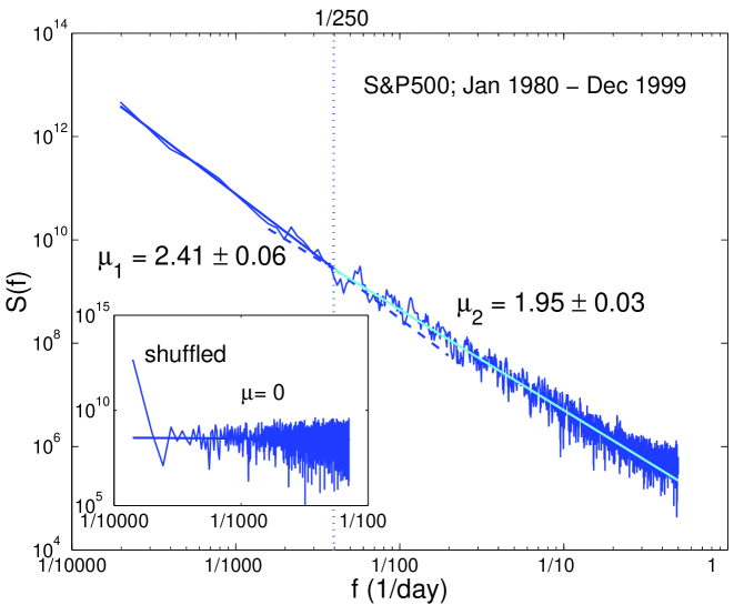
Figure 5: Power spectrum $S(f)$ of the daily closing price value signal of S&P500 between Jan. 01, 1980 and Dec. 31, 1999. A scale break at around $f=1/250$ day^-1 separates two scaling regions. Inset: Scaling of the power spectrum of the daily closing price signal of S&P500 as a white noise signal with $\mu\approx 0$

The power spectrum of the daily closing price signal of S&P500 $S(f)\sim f^{-\mu}$ with spectral exponents $\mu_{1}=2.41\pm 0.06$ and $\mu_{2}=1.95\pm 0.03$ with a scale break at 250 days is shown in Fig. 5. The scaling properties of the power spectrum of the shuffled daily closing price signal of S&P500, in which e.g. the amplitudes are randomly shuffled are shown in the inset of Fig. 5. Such a scaling spectral exponent $\mu=0$ is the signature of a white noise like behavior. Recall that $\mu=2.0$ corresponds to Brownian motion.

We have also checked for scaling behavior and possible periodicities in the power spectrum of the time series of the normalized log returns $Z(t,\Delta t)=(\tilde{y}(t)-<\tilde{y}>_{\Delta t})/\sigma_{\Delta t}$ for different (selected) values of the time lag $\Delta t=1,5,20,35,$ $40$ days (Fig. 6). A white noise like behavior of the power spectrum of such returns always occurs for $1/f$ $\leq$ $\Delta t$ days; e.g., dashed line in Fig. 6 for $f<1/128$ and $\Delta t=40$ days. This is in accordance with the results of the DFA analysis (Fig. 4 and Table 2). A scaling behavior is found at large frequencies $f$ satisfying the relationship $\mu=2H_{DFA}+1$, as indicated in Fig. 6, e.g. by the dashed line with slope $\mu=1.86$, for $f>1/128$ for the case $\Delta t=40$ days.

Periodicities in the power spectrum of the normalized log return time series for $\Delta t>1$ day were expected to be found since these periods are somewhat embedded into the time series by the way they are obtained and the Fourier transform technique. It is easily observed that the maxima and the minima of the spectrum correspond to harmonics and subharmonics of $1/\Delta t$.

4 Tsallis statistics

Based on the scaling properties of multifractals [40], Tsallis [15, 41] proposed a generalized Boltzmann-Gibbs thermo-statistics through the introduction of a family of non-extensive entropy functional ${\cal S}_{q}$ given by:

$${\cal S}_{q}=k\frac{1}{q-1}\left(1-\int p(x,t)^{q}dx\right),$$ (3)

with a single parameter $q$ and where $k$ is a normalization constant. The main ingredient in Eq.(3) is the time-dependent probability distribution $p(x,t)$ of the stochastic variable $x$. The functional is reduced to the classical extensive Boltzmann-Gibbs form in the limit of $q\longrightarrow 1$. The Tsallis parameter $q$ characterizes the non-extensivity of the entropy. Subject to certain constraints the functional in Eq.(3) seems to yield a probability distribution function of the form [6, 15, 19, 24, 27]

$$p(x)=\frac{1}{Z_{q}}\left\{1+\frac{C\beta_{0}2\alpha(q-1)|x|^{2\alpha}}{2\alpha-(q-1)}\right\}^{-\frac{1}{(q-1)}}$$ (4)

for the stochastic variable $x$, where

$$\frac{1}{Z_{q}}=\alpha\left\{\frac{C\beta_{0}2\alpha(q-1)}{2\alpha-(q-1)}\right\}^{1/2\alpha}\,\frac{\Gamma\left(\frac{1}{q-1}\right)}{\Gamma\left(\frac{1}{2\alpha}\right)\Gamma\left(\frac{1}{q-1}-\frac{1}{2\alpha}\right)}$$ (5)

in which $C$ is a constant and $0<\alpha\leq 1$ is the power law exponent of the potential $U(x)=C|x|^{2\alpha}$ that provides the ”restoring force” $F(x)$ in Beck model of turbulence [19, 20, 21, 23]. The latter is described by a Langevin equation

$$\frac{dx}{dt}=-\gamma F(x)+R(t)$$ (6)

where $\gamma$ is a parameter and $R(t)$ is a gaussian white noise. A non-zero value of $\gamma$ corresponds to providing energy to (or draining from) the system by the outside [42] The parameter $\beta_{0}$ in Eq.(4) and (5) is the mean of the fluctuating volatility $\beta$, i.e. the local standard deviation of $|x|$ over a certain window of size $m$ [6]. We will use this model assuming that the normalized log returns $Z(t,\Delta t)$ represent $the$ stochastic variable $x$, as in Eq.(6), or $\Delta y$ in Eq.(1). We will search whether Eq.(4) is obeyed for $x\equiv Z(t,\Delta t)$, thus studying $p(x)\equiv p_{\Delta t}(Z)$ for various time lags $\Delta t$.

Just as in Beck model of turbulence [19, 20, 21] we assume that the volatility $\beta$ is $\chi^{2}$-distributed with degree $\nu$ (see another formula in [23]):

$$f_{\Delta t}(\beta)\equiv\frac{1}{\Gamma(\nu/2)}\left(\frac{\nu}{2\beta_{0}}\right)^{\nu/2}\beta^{\nu/2-1}\exp\left(-\frac{\nu\beta}{2\beta_{0}}\right),\quad\nu>2,$$ (7)

where $\Gamma$ is the Gamma function, $\beta_{0}=<\beta>$ and the number of degrees of freedom $\nu$ can be found from:

$$\nu=\frac{2<\beta>^{2}}{<\beta^{2}>-<\beta>^{2}}.$$ (8)

The Tsallis parameter $q$ satisfies [19]

$$q\equiv 1+\frac{2\alpha}{\alpha\nu+1}.$$ (9)

To justify our assumption that the ’local’ volatility of the normalized log returns $Z(t,\Delta t)$ is of the form of $\chi^{2}$-distribution, we checked the distribution of the normalized log returns of the daily closing price of S&P500. We have calculated the standard deviation of the normalized log returns within various non-overlapping windows of size $m$, ranging from 25 to 1000  days

$$\beta(k)=\sqrt{{1\over m}\sum_{i=km+1}^{(k+1)m}Z^{2}(i)-\left({1\over m}\sum_{i=km+1}^{(k+1)m}Z(i)\right)^{2}}$$ (10)

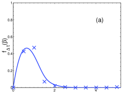
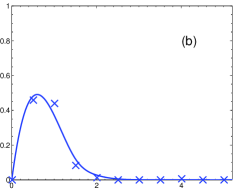
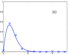
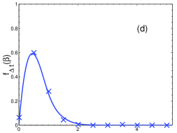
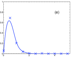
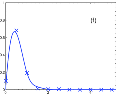
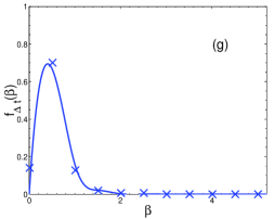
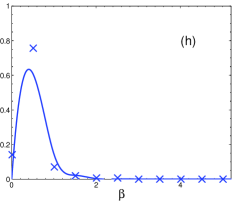
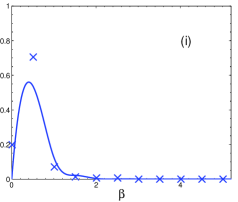
Figure 7: Probability density $f_{\Delta t}(\beta)$ of the local volatility $\beta$ (Eq.(10)) in terms of standard deviation of the normalized log returns $Z(t,\Delta t)$ of S&P500 in non-overlapping windows with size $m$=32 days for different time lags (symbols) (a-i) $\Delta t=$1, 5, 10, 15, 20, 25, 30, 35, 40 days. Lines: $\chi^{2}$-distribution as given by Eq. (7)

In doing so we have a various number of ${\cal M}$ non-overlapping windows for various time lags $\Delta t$, and have searched for the most efficient size of the window in order not to loose data points and therefore information. The resulting empirically obtained distributions of the ’local’ volatility (Eq.(10)) of normalized log returns for the different different time lags of interest are plotted in Fig. 7 for an intermediary case $m=32$. The values of the degree $\nu$ of the $\chi^{2}$-distribution are then obtained using Eq. (8). The spread $[\beta_{min},\beta_{max}]$ of the local volatility $\beta$ decreases with increasing the time lag as it is expected from a $\chi^{2}$-distribution function due to the exponential function in Eq. (7) for large values of the degree of freedom $\nu$. The value of $\nu$ much varies as a function of $m$ and the time lags considered. The fits are always excellent. However the $\beta_{0}$ and $\nu$ values are quite dependent on the parameters used in the numerical analysis. Based on these results, e.g. Fig. 7, it can be accepted that the (turbulent market) model $\beta$-distributions can be sufficiently well fitted for our purpose with a $\chi^{2}$-distribution, thereby justifying the initial assumption.

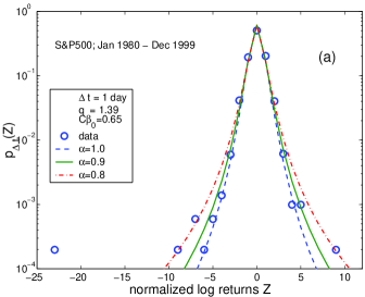
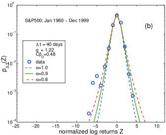
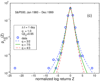
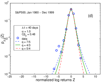
Figure 8: Probability distribution functions of the normalized log returns of daily closing price signal of S&P500 (symbols) for (a) $\Delta t=1$ day and fixed $q=1.39$. The Tsallis type distribution functions (Eq.(4)) obtained for various values of the parameter $\alpha=1.0,0.9,0.8$, dashed, solid, dash-dotted line, respectively; (b) same as (a) but for $\Delta t=40$ days and $q=1.22$; (c) for $\Delta t=1$ day and fixed $\alpha=1.0$ for various values of $q=3/2,7/5,4/3$, dashed, solid, dash-dotted line, respectively; (d) same as (c) but for $\Delta t=40$ days and $q=7/5,4/3,5/4$

In order to investigate the impact of the $\alpha$ parameter on the tail behavior of the Tsallis type distribution function we tested Eq. (4) for fixed $q$ in two cases : for a time lag $\Delta t=1$ day and $q=1.39$ (Fig. 8a) and for a time lag $\Delta t=40$ days and $q=1.22$ for $\alpha=1,0.9,0.8$ (Fig. 8b). Next we tested Eq. (4) for fixed $\alpha=1$ and varying $q$ : for a time lag $\Delta t=1$ day and for $q=3/2,7/5,4/3$ (Fig. 8c) and for a time lag $\Delta t=40$ days for $q=7/5,4/3,5/4$ (Fig. 8d). As expected the tails of the distribution functions approach a Gaussian type when $q$ is approaching 1. For completeness, the corresponding cases of the distribution of price increments are shown and briefly discussed in the Appendix.

In so doing the probability distributions of the normalized log returns for the different values of the time lag $\Delta t=1,5,10,15,20,25,30,35,40$ days can be shown in Fig. 2 together with the lines representing the best fit to the Tsallis type of distribution function. In Table 3 the statistical parameters related to the Tsallis type of distribution function are summarized, including a criterion for the goodness of the fit, i.e. the Kolmogorov-Smirnov distance $d_{KS}$, which is defined as the maximum distance between the cumulative probability distributions of the data and the fitting lines. Note that the kurtosis (see Table 3) for the Tsallis type of distribution function

$$K_{r}=K_{L}\frac{(5-3q)}{(7-5q)},$$ (11)

where $K_{L}=3$ for a Gaussian process, is positive for all values of $q<7/5$ as expected, since its positiveness is directly related to the occurrence of intermittency [6]. Moreover, the limit $q<7/5$ also implies that the second moment of the Tsallis type distribution function will always remain finite, as necessarily due in the type of phenomena hereby studied. Furthermore, if we assume that the Kolmogorov log-normal model of turbulence [47] is applicable and let $\Delta t_{L}$ be the scale at which the $whole$ partial distribution function becomes Gaussian, then the kurtosis $K_{r}$ should scale as

$$K_{r}=K_{L}\left(\frac{\Delta t}{\Delta t_{L}}\right)^{-\delta}.$$ (12)

Therefore

$$q=\frac{5-7\left(\Delta t/\Delta t_{L}\right)^{-\delta}}{3-5\left(\Delta t/\Delta t_{L}\right)^{-\delta}}.$$ (13)

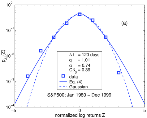
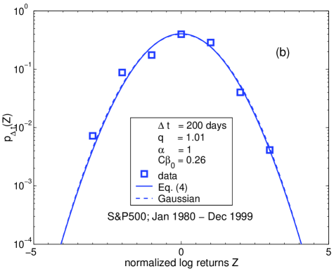
Figure 9: Partial distribution function of normalized log return of daily closing price of S&P500 for a large time lag, i.e. (a) $\Delta t=120$ days and (b) $\Delta t=200$ days. The solid line marks the best fit with a Tsallis type distribution function, Eq. (4), while the Gaussian distribution function is drawn with a dashed line

In order to obtain an estimate for $\Delta t_{L}$, we observe that the turbulence model, Eq. (4), fits well the normalized log returns for $\Delta t=120$ days and $q=1.01$ (Fig. 9a). The $\alpha$-parameter ($\alpha=0.74$) in this case plays an important role in controlling the tails such that the Tsallis type distribution function for negative values of $Z$ fits the data whose probability distribution function still deviates from Gaussian. In fact, further increasing the time lag to the value $\Delta t=200$ days leads to a complete coincidence between the distribution functions in the Tsallis and Gaussian forms for the presently investigated data (Fig. 9b). Corresponding parameter values are also listed in Table 3. This short observation convincingly indicates where the transition occurs between the small time scale model of nonextensive, intermittent process and the large scale Gaussian extensive homogeneous fluctuation picture [6, 15] and refine the estimate of the Gaussian range in Figs.1-2.

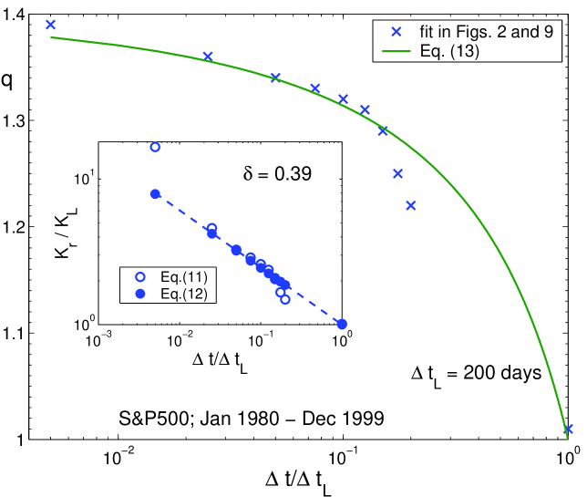
Figure 10: The functional dependence of the Tsallis $q$ parameter on the rescaled time lag $\Delta t/\Delta t_{L}$ for $\Delta t_{L}=200$ days and $\delta=0.39$ (see Eq. (13)) (line); the symbols represent the values of the $q$ parameter listed in Table 3 and used to plot the fitting lines in Figs. 2 and 9. Inset : Scaling properties of the rescaled kurtosis $K_{r}/K_{L}$, where $K_{L}=3$ is the kurtosis for a Gaussian process, as a function of the rescaled time lag $\Delta t/\Delta t_{L}$ satisfying Eq. (11) (open symbols) and Eq. (12) (full symbols)

In Fig. 10 the Tsallis parameter $q$ is shown as a function of the rescaled time lags $\Delta t/\Delta t_{L}$, where $\Delta t_{L}$ is the integral scale, the scale at which the $whole$ probability distribution function converges to Gaussian. The crosses) represent the $q$ values for which the best fit to the S&P500 data (Fig. 2) is obtained with Eq. (4). With this the value of the integral scale $\Delta t_{L}$, we find the value of the exponent $\delta=0.39$ as the one for which the Eq. (13) fits best the $q$-values. The exponent value $\delta=0.39$ also allows to fit well the power law dependence (Eqs. (11) and (12)) of the rescaled kurtosis $K_{r}/K_{L}$ as shown in the inset of Fig. 10.

Note that in the framework of the Kolmogorov log-normal model [47, 20], $\delta=4\kappa/9$, where $\kappa$ is called the intermittency exponent. Therefore, we find $\kappa=0.88$ for the intermittency exponent of normalized log returns of the S&P500 daily closing price in the time interval of interest. This value of $\kappa$ is higher than the value of the intermittency exponent $\kappa=0.25$ for turbulence recently obtained from experimental atmospheric data [48]. Early estimates have varied from 0.18 to 0.85 using different experimental techniques [49, 50, 51]. Large values of the intermittency exponent, ranging from 0.2 to 0.8, have been reported in studies of multiparticle production [52]. It was found that the range of intermittency exponent values depend on the number of cascades; the smaller the number of stages of the multiplicative cascade the smaller $\kappa$, and conversely [Fig. 2b in [52]]. In analogy with such findings, a value of $\kappa=0.88$ can be considered to be related to a high number of cascades in a multiplicative process, leading to the observed partial distribution functions of the normalized log returns of the S&P500 index.

One can explore the Tsallis type of the probability distribution function Eq.(4) in two limits. For small values of normalized log returns $Z$ the probability distribution function converges to the form

$$p_{\Delta t}(Z)\approx\frac{1}{Z_{q}}\exp\left\{-\frac{C\beta_{0}2\alpha}{2\alpha-(q-1)}|Z|^{2\alpha}\right\}$$ (14)

Therefore the Tsallis type distribution function converges to a Gaussian, i.e. $\alpha\longrightarrow 1$, for small values of the normalized log returns, for any $\Delta t$ investigated hereby (see Figs. 1-2). It is also of interest to check the probability of return to the origin $p_{\Delta t}(Z=0)$ (Table 3). There is a slight difference between the values of the probability of ”return to the origin” for the data and the one obtained from Eq.(4) $p_{\Delta t}(Z=0)=1/Z_{q}$. This difference is decreasing with increasing $\Delta t$ and completely disappears in the Gaussian limit $q\longrightarrow 1$, $\alpha\longrightarrow 1$.

In the limit of large values of normalized log returns $Z$, the Tsallis type distribution converges to a power law

$$p_{\Delta t}(Z)\approx\frac{1}{Z_{q}}\left\{\frac{(q-1)C\beta_{0}2\alpha}{2\alpha-(q-1)}|Z|^{2\alpha}\right\}^{-\frac{1}{q-1}.}$$ (15)

Studying the Tsallis type of distribution function one can obtain from Eq.(4) an expression for the width of the Tsallis type of probability distribution function, $2\sigma_{w}^{2}=(2\alpha-(q-1))/(2\alpha C\beta_{0}(q-1))$. In the limit of $\alpha\longrightarrow 1$ the width of the Tsallis type distribution $2\sigma_{w}^{2}=(3-q)/2C\beta_{0}(q-1)$, i.e. $\sim 2/(C\beta_{0})$. It is obvious that for large time lags $2\sigma^{2}_{w}$ tends to diverge [24], like $\simeq(\Delta t)^{2/(3-q)}$; this can be easily verified on a log-log plot (not shown).

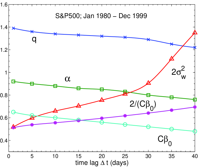
Figure 11: Characteristic parameters of Tsallis type distribution function as defined in [27] : Tsallis $q$-parameter (crosses), $\alpha$ (squares), constant $C\beta_{0}$ used in the fit (open circles), the width of the Tsallis type distribution $2\sigma_{w}^{2}=(2\alpha-(q-1))/(2\alpha C\beta_{0}(q-1))$ from Eq.(4) (triangles) (rescaled by a factor of 1/6), asymptotic behavior of $2\sigma_{w}^{2}\approx 2/(C\beta_{0})$ for $\alpha\longrightarrow 1$ (full circles) (rescaled by a factor of 1/6)

In limit of $q\longrightarrow 1$ the Tsallis type distribution function converges to Gaussian (as seen in Fig. 9b). The values of the parameters $q$, $\alpha$, $C\beta_{0}$, that best fit the data using Eq.(4), and $2\sigma_{w}^{2}$ are plotted as a function of the time lag in Fig. 11.

5 Fokker-Planck approach

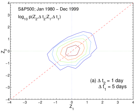
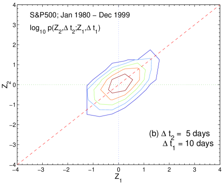
Figure 12: Typical contour plots of the joint probability density function $p(Z_{2},\Delta t_{2};Z_{1},\Delta t_{1})$ of daily closing price of S&P500 for the period of interest Jan. 01, 1980 and Dec. 31, 1999. Dashed lines have a slope +1 and emphasize the correlations between probability density functions for (a) $\Delta t_{2}=1$ day and $\Delta t_{1}=5$ days and (b) $\Delta t_{2}=5$ days and $\Delta t_{1}=10$ days. Contour levels correspond to $log_{10}p(Z_{2},\Delta t_{2};Z_{1},\Delta t_{1})=-1.0,-1.5,-2.0,-2.5,-3.0$ from center to border

On the other hand, the evolution of a time dependent probability distribution function is usually described within the Fokker-Planck approach. This method provides some further information on the correlations present in the time series and it begins with the joint PDF’s, that depend on $\cal{N}$ variables, i.e. $p^{\cal{N}}(Z_{1},\Delta t_{1};...;Z_{\cal{N}},\Delta t_{\cal{N}})$. We started to address this issue by determining the joint PDF for ${\cal{N}}=2$, i.e. $p(Z_{2},\Delta t_{2};\Delta x_{1},\Delta t_{1})$. The symmetrically tilted character of the joint PDF contour levels (Fig. 12) around an inertia axis with slope 1/2 points out to some statistical dependence, i.e. a correlation, between the normalized log returns $Z(t,\Delta t)$ of the daily closing price signal of S&P500. A lack of correlations would put the inertia axis on the main diagonal (Fig. 12).

The conditional probability function is

$$p(Z_{i+1},\Delta t_{i+1}|Z_{i},\Delta t_{i})=\frac{p(Z_{i+1},\Delta t_{i+1};Z_{i},\Delta t_{i})}{p(Z_{i},\Delta t_{i})}$$ (16)

for $i=1,...,{\cal{N}}-1$. For any $\Delta t_{2}$ $<$ $\Delta t_{i}$ $<$ $\Delta t_{1}$, the Chapman-Kolmogorov equation is a necessary condition of a Markov process, one without memory but governed by probabilistic conditions

$$p(Z_{2},\Delta t_{2}|Z_{1},\Delta t_{1})=\int d(Z_{i})p(Z_{2},\Delta t_{2}|Z_{i},\Delta t_{i})p(\Delta x_{i},\Delta t_{i}|Z_{1},\Delta t_{1}).$$ (17)

The Chapman-Kolmogorov equation when formulated in $differential$ form yields a master equation, which can take the form of a Fokker-P1anck equation [43]. Let $\tau=log_{2}(200/\Delta t)$,

$$\frac{d}{d\tau}p(Z,\tau)=\left[-\frac{\partial}{\partial Z}D^{(1)}(Z,\tau)+\frac{\partial}{\partial Z^{2}}D^{(2)}(Z,\tau)\right]p(Z,\tau)$$ (18)

in terms of a drift $D^{(1)}$($Z$,$\tau$) and a diffusion coefficient $D^{(2)}$($Z$,$\tau$) (thus values of $\tau$ represent $\Delta t_{i}$, $i=1,...$).

The coefficient functional dependence can be estimated directly from the moments $M^{(k)}$ (known as Kramers-Moyal coefficients) of the conditional probability distributions:

$$M^{(k)}=\frac{1}{\Delta\tau}\int dZ^{{}^{\prime}}(Z^{{}^{\prime}}-Z)^{k}p(Z^{{}^{\prime}},\tau+\Delta\tau|Z,\tau)$$ (19)

$$D^{(k)}(Z,\tau)=\frac{1}{k!}\mbox{lim}M^{(k)}$$ (20)

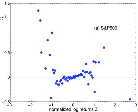
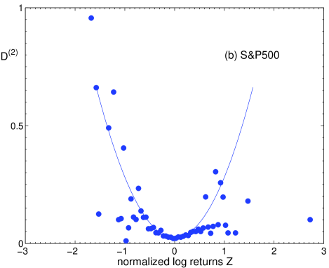
Figure 13: Kramers-Moyal drift and diffusion coefficients (a) $D^{(1)}$ and (b) $D^{(2)}$ as a function of normalized log returns $Z$ for daily closing price of S&P500 ; $D^{(2)}=0.26Z^{2}-0.0005Z+0.02$

for $\Delta\tau\rightarrow 0$. According to Fig. 13a the drift coefficient $D^{(1)}\approx 0$ and the diffusion coefficients $D^{(2)}$ is well represented (Fig. 13b) by a parabola

$$D^{(2)}(Z)=0.26Z^{2}-0.005Z+0.02$$ (21)

in the interval $Z\in[-0.175,0.225]$, - noticing that it is smaller than the one presented in Fig.2.

It may be worthwhile to recall that the observed quadratic dependence of the diffusion term $D^{(2)}$ is essential for the logarithmic scaling of the intermittency parameter in studies on turbulence.

Finally, the Fokker-Planck equation for the distribution function is known to be equivalent to a Langevin equation for the variable, i.e. $Z$ here, (within the Ito interpretation [7, 43, 44, 45, 46])

$$\frac{d}{d\tau}Z(\tau)=D^{(1)}(Z(\tau),\tau)+\eta(\tau)\sqrt{{D^{(2)}(Z(\tau),\tau)}},$$ (22)

where $\eta(\tau)$ is a fluctuating $\delta$-correlated force with Gaussian statistics, i.e. $<$ $\eta(\tau)$ $\eta(\tau^{\prime})$$>$ = 2$\delta(\tau-\tau^{\prime})$.

Thus the Fokker-Planck approach provides the evolution process of PDF’s from small time lags to larger ones. The fact that the drift coefficient is approximately equal to zero, therefore indicating that there is no correlation between the probability distribution functions for different time lags, is well related to the Gaussian character of the distribution function for such small values of the normalized log returns $Z\in[-3,3]$. $D^{(1)}\approx 0$ further implies that there is almost no ”restoring force”, i.e. $\gamma\approx 0$ in Eq. (6), while the quadratic dependence of $D^{(2)}$ in $Z$ is obviously like an autocorrelation function for a diffusion process.

6 Conclusion

In summary, we have presented a method that provides the evolution process of probability distribution functions (over twenty years) of one financial index, i.e. the S&P500. We have studied the evolution process of the tails that are outside the central (Gaussian) regime at small returns, thereby facilitating the understanding of the evolution of these distribution functions in a Fokker-Planck framework. Beck turbulence model can be well applied to describe the volatility (of normalized log-returns) distributions assuming a $\chi^{2}$-distribution for the ”local” volatility. An open question in nonextensive thermostatistics studies is often raised about the meaning, value and behavior of the non extensive exponent, or Tsallis parameter $q$. The intermittency exponent is found to be related to the scaling exponent of the PDF moments in the framework of Kolmogorov log-normal model, thereby giving weight to the model and the statistical approach. The intermittency exponent large value points to a large number of cascades in the turbulent process. Its range has been found to extend up to $ca.$ 200 days. One may still wonder on the $q$-value itself. In other works, this value is related, e.g. to the upper and lower bounds of the multifractal dimension [17], in other words to the bounds of the $\alpha$ values in multifractal studies [40]. It may also be related to the value of the fractional derivative, say in a non-linear Fokker-Planck equation approach [53]. This should be some interesting work to pursue, - again with some warning concerning the possible error bars on the generalized fractal dimension in multifractal studies [54].

We have also presented the turbulence-like dynamics through the Fokker-Planck and the Langevin equations. We have (unexpectedly) found that, in the treated case, there is almost no ”restoring force”, i.e. ($\gamma\approx 0$ in the Langevin equation). A comparison is made between normalized log-returns and mere price increments. We have examined the corresponding cases of the distribution of price increments with other possible definitions. It was found that the definition (through a normalized log return rather than a mere price difference) is very relevant for obtaining nice fits. This has been also observed in a work by Karth and Peinke [55] on related matter. This warning might also shine some light on the possible origin of the controversy [4, 5] concerning the relationship (or not) between the fat tails caused by some dynamical hierarchical cascade process of volatility correlations.

These points not withstanding, we have related a financial market behavior to Tsallis non extensive thermodynamics approach, i.e. more precisely to a turbulence-like process, - as financial market and indices were often claimed to be seen [2, 12, 13]. Finally, it seems that we have thoroughly answered the often raised question ”why to look at the tails of a probability distribution function? and what does that lead to?”.

7 Appendix

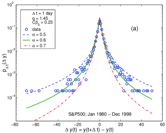
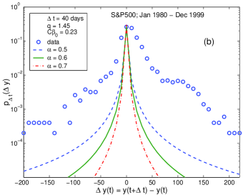
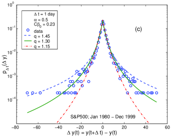
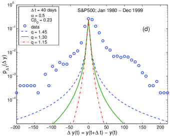
Figure 14: Probability distribution functions of the daily closing price increments $\Delta y(t)=y(t+\Delta t)-y(t)$ of S&P500 (symbols). The Tsallis type distribution functions (Eq.(4)) obtained (a) for $\Delta t=1$ day and fixed $q=1.45$ ($C\beta_{0}=0.23$) and for various values of the parameter $\alpha=0.5,0.6,0.7$, dashed, solid, dash-dotted line, respectively; (b) the same as (a) but for $\Delta t=40$ days; (c) for $\Delta t=1$ day and fixed $\alpha=0.5$ ($C\beta_{0}=0.23$) and for various values of $q=1.45,1.30,1.15$, dashed, solid, dash-dotted line, respectively; (d) the same as (b) but for $\Delta t=40$ days

We have also searched for describing the partial distribution function of the (raw) increments of daily closing price signal of the S&P500 with the Tsallis type distribution function. We have applied Eq.(4) for $x\equiv\Delta y(t,\Delta t)=y(t+\Delta t)-y(t)$. We have tested the Tsallis type distribution function for the increments of $\Delta t=1$ day for fixed $q=1.45$ ($C\beta_{0}=0.23$) and varying $\alpha=0.5,0.6,0.7$ (Fig. 14a). Applying the same set of parameters and to price increments for $\Delta y=40$ days, leads to a pretty bad fit (Figs. 14b). Decreasing the value of $q$ would not have produce better results since the Tsallis type distribution function would have been bounded within smaller range around $\Delta y=0$ values. A test for fixed $\alpha=0.5$ ($C\beta_{0}=0.23$) and varying $q=1.45,1,30,1.15$ for $\Delta t=1$ day is next shown in Fig. 14c. Again the same set of parameters is applied to price increments for $\Delta y=40$ days and lead to a pretty bad fit (Figs. 14d). These results may be somewhat expected because the Tsallis type distribution function represents a mathematical construction that is designed for normalized variables, i.e. a variable changing within a limited range. To take into account a double peak like structure (e.g. for large time lags, see Fig.14) remains an open question.

Figure Captions

Figure 1 – Probability distribution function of normalized log returns $Z(t,\Delta t)$ of daily closing price value signal of S&P500 between Jan. 01, 1980 and Dec. 31, 1999, for $\Delta t=1$ day (symbols). Normalized log returns are calculated as $Z(t,\Delta t)=(\tilde{y}(t)-<\tilde{y}>_{\Delta t})/\sigma_{\Delta t}$, where $\tilde{y}(t)=ln(y(t+\Delta t)/y(t))$ and $\sigma_{\Delta t}$ is the standard deviation of $\tilde{y}(t)$ for time lag $\Delta t$. The dashed line represents a Gaussian distribution. Inset: Power law fit (solid line) of the negative (-3.1) and positive (-3.1) slope of the distribution outside the Gaussian regime

Figure 2 – Probability distribution function (PDF) $p_{\Delta t}(Z)$ of normalized log returns of the daily closing price value signal of S&P500 (symbols) and the Tsallis type distribution function (lines) for different values of $\Delta t=1,5,10,15,20,25,30,35,40$ days. The PDF (symbols and curves) for each $\Delta t$ are displaced by 10 with respect to the previous one; the curve for $\Delta t=1$ day is unmoved. The large circles mark the ends of the interval in which the distribution is $like$ a gaussian distribution. The values of the slopes of the positive and negative tails of the distributions outside the gaussian range $Z\in[-3,3]$ are listed in Table 1. The values of the parameters for the Tsallis type distribution function for each $\Delta t$ are summarized in Table 3

Figure 3 – DFA function $F(n)$ plotted as a function of the the box size $n$ of the integrated daily closing price value signal of S&P500 between Jan. 01, 1980 and Dec. 31, 1999. Brownian-like fluctuations with $1+H_{DFA}=1.52\pm 0.01$ are obtained for all possible time scales

Figure 4 – DFA function $F(n)$ plotted as a function of the the box size $n$ of the integrated normalized log returns $Z(t,\Delta t)$ of daily closing price value signal of S&P500 between Jan. 01, 1980 and Dec. 31, 1999 for different time lags $\Delta t=1,5,10,15,20,25,30,35,40$ days. Values of the scaling exponents $H_{DFA}$ for the various DFA functions are summarized in Table 2. Inset: Power law functional dependence of the value of the cross over box-size $n_{x}$ as a function of time lag $\Delta t$

Figure 5 – Power spectrum $S(f)$ of the daily closing price value signal of S&P500 between Jan. 01, 1980 and Dec. 31, 1999. A scale break at around $f=1/250$ day^-1 separates two scaling regions. Inset: Scaling of the power spectrum of the daily closing price signal of S&P500 as a white noise signal with $\mu\approx 0$

Figure 6 – Power spectrum $S(f)$ of the normalized log returns $Z(t,\Delta t)$ of daily closing price value signal of S&P500 between Jan. 01, 1980 and Dec. 31, 1999 for different time lags $\Delta t=1,5,20,35,40$ days. Each curve is displaced by $10^{-5}$ with respect to the previous one; the power spectrum of the normalized log returns for $\Delta t=1$ day is not displaced. The dashed line from $f=1/70$ days^-1 to $f=1/2$ days^-1 has a slope $\mu=1.86$, corresponding to the $H_{DFA}$ exponent. The horizontal dashed line from $f=1/10^{-4}$ days^-1 to $f=1/128$ days^-1 corresponds to what should be expected for white noise and is in agreement with the scaling of the DFA function for the same data in Fig. 4

Figure 7 – Probability density $f_{\Delta t}(\beta)$ of the local volatility $\beta$ (Eq.(10)) in terms of standard deviation of the normalized log returns $Z(t,\Delta t)$ of S&P500 in non-overlapping windows with size $m$=32 days for different time lags (symbols) (a-i) $\Delta t=$1, 5, 10, 15, 20, 25, 30, 35, 40 days. Lines: $\chi^{2}$-distribution as given by Eq. (7).

Figure 8 – Probability distribution functions of the normalized log returns of daily closing price signal of S&P500 (symbols) for (a) $\Delta t=1$ day and fixed $q=1.39$. The Tsallis type distribution functions (Eq.(4)) obtained for various values of the parameter $\alpha=1.0,0.9,0.8$, dashed, solid, dash-dotted line, respectively; (b) same as (a) but for $\Delta t=40$ days and $q=1.22$; (c) for $\Delta t=1$ day and fixed $\alpha=1.0$ for various values of $q=3/2,7/5,4/3$, dashed, solid, dash-dotted line, respectively; (d) same as (c) but for $\Delta t=40$ days and $q=7/5,4/3,5/4$

Figure 9 – Partial distribution function of normalized log return of daily closing price of S&P500 for a large time lag, i.e. (a) $\Delta t=120$ days and (b) $\Delta t=200$ days. The solid line marks the best fit with a Tsallis type distribution function, Eq. (4), while the Gaussian distribution function is drawn with a dashed line

Figure 10 – The functional dependence of the Tsallis $q$ parameter on the rescaled time lag $\Delta t/\Delta t_{L}$ for $\Delta t_{L}=200$ days and $\delta=0.39$ (see Eq. (13)) (line); the symbols represent the values of the $q$ parameter listed in Table 3 and used to plot the fitting lines in Figs. 2 and 9. Inset : Scaling properties of the rescaled kurtosis $K_{r}/K_{L}$, where $K_{L}=3$ is the kurtosis for a Gaussian process, as a function of the rescaled time lag $\Delta t/\Delta t_{L}$ satisfying Eq. (11) (open symbols) and Eq. (12) (full symbols)

Figure 11 – Characteristic parameters of Tsallis type distribution function as defined in [27] : Tsallis $q$-parameter (crosses), $\alpha$ (squares), constant $C\beta_{0}$ used in the fit (open circles), the width of the Tsallis type distribution $2\sigma_{w}^{2}=(2\alpha-(q-1))/(2\alpha C\beta_{0}(q-1))$ from Eq.(4) (triangles) (rescaled by a factor of 1/6), asymptotic behavior of $2\sigma_{w}^{2}\approx 2/(C\beta_{0})$ for $\alpha\longrightarrow 1$ (full circles) (rescaled by a factor of 1/6)

Figure 12 – Typical contour plots of the joint probability density function $p(Z_{2},\Delta t_{2};Z_{1},\Delta t_{1})$ of daily closing price of S&P500 for the period of interest Jan. 01, 1980 and Dec. 31, 1999. Dashed lines have a slope +1 and emphasize the correlations between probability density functions for (a) $\Delta t_{2}=1$ day and $\Delta t_{1}=5$ days and (b) $\Delta t_{2}=5$ days and $\Delta t_{1}=10$ days. Contour levels correspond to $log_{10}p(Z_{2},\Delta t_{2};Z_{1},\Delta t_{1})=-1.0,-1.5,-2.0,-2.5,-3.0$ from center to border

Figure 13 – Kramers-Moyal drift and diffusion coefficients (a) $D^{(1)}$ and (b) $D^{(2)}$ as a function of normalized log returns $Z$ for daily closing price of S&P500 ; $D^{(2)}=0.26Z^{2}-0.0005Z+0.02$

Figure 14 – Probability distribution functions of the daily closing price increments $\Delta y(t)=y(t+\Delta t)-y(t)$ of S&P500 (symbols). The Tsallis type distribution functions (Eq.(4)) obtained (a) for $\Delta t=1$ day and fixed $q=1.45$ ($C\beta_{0}=0.23$) and for various values of the parameter $\alpha=0.5,0.6,0.7$, dashed, solid, dash-dotted line, respectively; (b) the same as (a) but for $\Delta t=40$ days; (c) for $\Delta t=1$ day and fixed $\alpha=0.5$ ($C\beta_{0}=0.23$) and for various values of $q=1.45,1.30,1.15$, dashed, solid, dash-dotted line, respectively; (d) the same as (b) but for $\Delta t=40$ days

Table 1: Slopes of the positive and negative tails (second and third column) of the distributions outside the Gaussian range $Z(t,\Delta t)\in[-3,3]$; values of characteristic Tsallis function parameters are given

$\Delta t$	positive	negative	$2q$	$1/(q-1)$	$\alpha$
1	3.1	3.1	2.78	2.564	0.92
5	3.1	3.0	2.72	2.778	0.90
10	3.0	2.7	2.68	2.941	0.88
15	3.0	2.6	2.66	3.030	0.86
20	2.9	2.5	2.64	3.125	0.85
25	2.9	2.5	2.62	3.226	0.83
30	2.8	2.3	2.58	3.448	0.80
35	2.7	2.3	2.50	4.000	0.78
40	2.5	2.2	2.44	4.545	0.76

Table 2: Values of the scaling exponent from the DFA analysis of normalized log returns $Z$ for different values of the time lag $\Delta t=5,10,15,20,25,30,35,40$ days, and crossover ”box size” $n_{x}$

$\Delta t$	$1+H_{DFA}$	$n_{x}$
5	1.27$\pm$0.04	19
10	1.37$\pm$0.02	35
15	1.39$\pm$0.02	49
20	1.38$\pm$0.02	70
25	1.38$\pm$0.02	91
30	1.41$\pm$0.01	108
35	1.43$\pm$0.01	117
40	1.43$\pm$0.01	128

Table 3: Values of the parameters characterizing the S&P500 daily closing price data between Jan. 1, 1980 and Dec. 31, 1999 in the nonextensive thermostatisitics approach. For the definition of the Kolmogorov-Smirnov distance $d_{KS}$ see the text

$\Delta t$	$q$	$\alpha$	$C\beta_{0}$	$p_{\Delta t}(Z=0)$	$p_{\Delta t}(Z=0)$	$K_{r}$	$d_{KS}$
				data	Eq.(4)
1	1.39	0.92	0.65	0.505	0.611	49.800	0.072
5	1.36	0.90	0.62	0.447	0.600	13.800	0.100
10	1.34	0.88	0.60	0.462	0.592	9.800	0.091
15	1.33	0.86	0.58	0.472	0.582	8.657	0.085
20	1.32	0.85	0.56	0.459	0.572	7.800	0.085
25	1.31	0.83	0.54	0.447	0.560	7.133	0.087
30	1.29	0.80	0.52	0.443	0.549	6.164	0.088
35	1.25	0.78	0.50	0.432	0.538	5.000	0.087
40	1.22	0.76	0.48	0.445	0.525	4.467	0.077
120	1.01	0.74	0.39	0.431	0.467	3.031	0.052
200	1.01	1.00	0.26	0.398	0.406	3.031	0.040

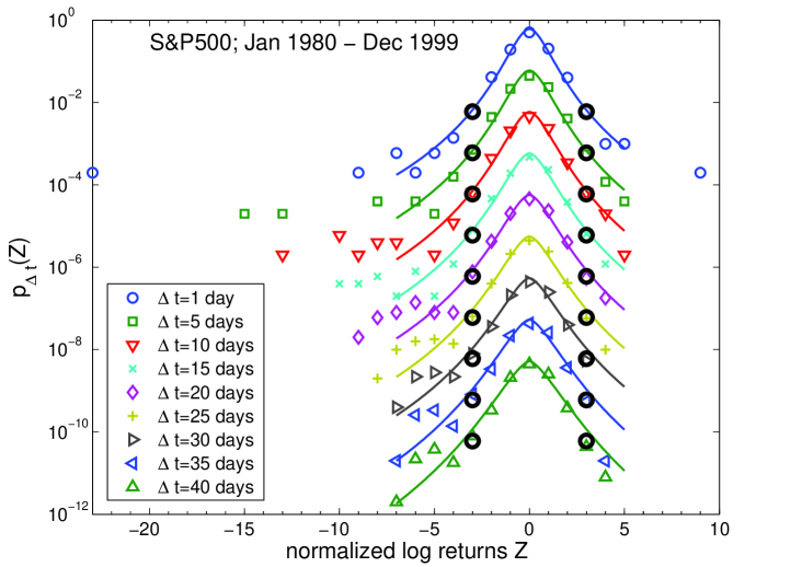
Figure 2: Probability distribution function (PDF) $p_{\Delta t}(Z)$ of normalized log returns of the daily closing price value signal of S&P500 (symbols) and the Tsallis type distribution function (lines) for different values of $\Delta t=1,5,10,15,20,25,30,35,40$ days. The PDF (symbols and curves) for each $\Delta t$ are displaced by 10 with respect to the previous one; the curve for $\Delta t=1$ day is unmoved. The large circles mark the ends of the interval in which the distribution is $like$ a gaussian distribution. The values of the slopes of the positive and negative tails of the distributions outside the gaussian range $Z\in[-3,3]$ are listed in Table 1. The values of the parameters for the Tsallis type distribution function for each $\Delta t$ are summarized in Table 3

References

- [1] E.F. Fama, J. Business 38, 34 (1965)
- [2] R.N. Mantegna, H.E. Stanley, An Introduction to Econophysics: Correlations and Complexity in Finance, Cambridge Univ. Press, Cambridge, 2000
- [3] R.N. Mantegna and H.E. Stanley, Nature 383, 587 (1996)
- [4] G. M. Viswanathan, U. L. Fulco, M. L. Lyra, and M. Serva, arXiv: cond-mat/ 0112484 v3
- [5] P. Gopikrishnan, V. Plerou, X. Gabaix, L.A.N. Amaral and H.E. Stanley, Physica A 299, 137 (2001); P. Gopikrishnan, V. Plerou, Y. Liu, X. Gabaix, L.A.N. Amaral and H.E. Stanley, Physica A 287, 362 (2000)
- [6] F.M. Ramos, R.R. Rosa, C. Rodrigues Neto, M.J.A. Bolzan and L.D. Abreu Sa, Nonlinear Analysis 47, 3521 (2001)
- [7] H. Risken, The Fokker-Planck Equation: Methods of Solution and Applications, 2nd edn, Springer-Verlag, Berlin, 1989
- [8] R. Friedrich, J. Peinke, and Ch. Renner, Phys. Rev. Lett. 84, 5224 (2000)
- [9] Ch. Renner, J. Peinke, and R. Friedrich, Physica A 298, 499 (2001)
- [10] F. Michael and M.D. Johnson, Physica A 324, 359 (2003)
- [11] K. Ivanova, M. Ausloos, and H. Takayasu, arXiv:cond-mat/0301268
- [12] S. Ghashghaie, W. Breymann, J. Peinke, P. Talkner, and Y. Dodge, Nature 381, 767 (1996)
- [13] F. Schmitt, D. Schertzer, and S. Lovejoy, in Chaos, Fractals and Models, F. M. Guindani and G. Salvadori, Eds., Italian University, Pavia, 1998, pp.150-157
- [14] U. Frisch, Turbulence: the Legacy of A. N. Kolmogorov, Cambridge Univ. Press, Cambridge, 1995
- [15] C. Tsallis, J. Stat. Phys. 52, 479 (1988)
- [16] C. Tsallis and D.J. Bukman, Phys. Rev. E 54, 2197 (1996)
- [17] G. Wilk and Z. Wlodarczyk, Phys. Rev. Lett. 84, 2770 (2000)
- [18] T. Arimitsu and N. Arimitsu, Prog. Theor. Phys. 105, 355 (2001)
- [19] C. Beck, Phys. Rev. Lett. 87, 180601 (2001)
- [20] C. Beck, Physica A 295, 195 (2001)
- [21] C. Beck, G. S. Lewis, and H. L. Swinney, Phys. Rev. E 63, 035303 (2001)
- [22] F. Sattin, arXives: cond-mat/0211157
- [23] F. Sattin, arXives: cond-mat/0212077
- [24] F. Michael and M.D. Johnson, Physica A 320, 525 (2003)
- [25] L. Borland, Phys. Rev. E 57, 6634 (1998); ibid. arXives: cond-mat/0205078; ibid. , arXives: cond-mat/0204331
- [26] H.M. Gupta and J.R. Campanha, Physica A 309, 381 (2002)
- [27] N Kozuki and N Fuchikami, arXives: cond-mat/0210090
- [28] C. Tsallis, C. Anteneodo, L. Borland, and R. Osorio, Physica A 324, 89 (2003)
- [29] N. Vandewalle and M. Ausloos, Physica A 246, 454 (1997)
- [30] N. Vandewalle and M. Ausloos, Phys. Rev. E 58, 6832 (1998)
- [31] D. Sornette, Why stock markets crash ? (Princeton University Press, January 2003), and references therein
- [32] N. Vandewalle and M. Ausloos, Eur. J. Phys. B 4, 139 (1998)
- [33] M.S. Taqqu, V. Teverovsky, and W. Willinger, Fractals 3, 785 (1995)
- [34] K. Hu, Z. Chen, P. Ch. Ivanov, P. Carpena, and H.E. Stanley, Phys. Rev E 64, 011114 (2001)
- [35] Sz. Mercik and K. Weron, Phys. Rev. E 63, 051910 (2001)
- [36] P. Ch. Ivanov, M. G. Rosenblum, C.-K. Peng, J. E. Mietus, S. Havlin, H. E.Stanley, and A. L. Goldberger, Nature 383, 323 (1996)
- [37] K. Ivanova and M. Ausloos, Physica A 274, 349 (1999)
- [38] K. Ivanova, M. Ausloos, E.E. Clothiaux, and T.P. Ackerman, Europhys. Lett. 52, 40 (2000)
- [39] E. Koscielny-Bunde, A. Bunde, S. Havlin, H. E. Roman, Y. Goldreich, and H.-J. Schellnhuber, Phys. Rev. Lett. 81, 729 (1998)
- [40] T.C. Halsey, M.H. Jensen, L.P. Kadanoff, I. Procaccia, and B.I. Shraiman, Phys. Rev. A 33, 1141 (1986)
- [41] C. Tsallis, S.V.F. Levy, A.M.C. Souza and R. Maynard, Phys. Rev. Lett. 75, 3589 (1995)
- [42] F. Sattin, J. Phys. A 36, 1583 (2003)
- [43] M.H. Ernst, L.K. Haines, and J.R. Dorfman, Rev. Mod. Phys. 41, 296 (1969)
- [44] L.E. Reichl, A Modern Course in Statistical Physics, Univ. Texas Press, Austin (1980)
- [45] P. Hänggi and H. Thomas, Phys. Rep. 88, 207 (1982)
- [46] C.W. Gardiner, Handbook of Stochastic Methods, Springer-Verlag, Berlin (1983)
- [47] A.M. Kolmogorov, J. Fluid Mech. 13, 82 (1962)
- [48] K.R. Sreenivasan and P. Kailasnath, Phys. Fluids 5, 512 (1993)
- [49] K.R. Sreenivasan, R.A. Antonia, and H.Q. Danh, Phys. Fluids 20, 1238 (1977)
- [50] R.R. Prasad, C. Meneveau, and K.R. Sreenivasan, Phys. Rev. Lett 61, 74 (1988)
- [51] J.C. Wyngaard and H. Tennekes, Phys. Fluids 13, 273 (1970)
- [52] R.A. Janik and B. Ziaja, Acta Phys. Pol. B 30, 259 (1999)
- [53] T.D. Frank, Physica A 320, 204 (2003); T. D. Frank and A. Daffertshofer, Physica A 292, 392 (2001); I.M. Sokolov, J. Klafter and A. Blumen, Phys. Today 55, (11) 48 (2002)
- [54] Th. Lux, Multi-Scaling Properties of Asset Returns: An Assessment of the Power of the ’Scaling Estimator’, Manuscript, University of Kiel, JEL classification: C20, G12, C15
- [55] M. Karth and J. Peinke, Complexity 8, 34 (2002)