Supersymmetry theory of microphase separation in homopolymer–oligomer mixtures

Abstract

Mesoscopic structure of the periodically alternating layers of stretched homopolymer chains surrounded by perpendicularly oriented oligomeric tails is studied for the systems with both strong (ionic) and weak (hydrogen) interactions. We focus on the consideration of the distribution of oligomers along the homopolymer chains that is described by the effective equation of motion with the segment number playing the role of imaginary time. Supersymmetry technique is developed to consider associative hydrogen bonding, self–action effects, inhomogeneity and temperature fluctuations in the oligomer distribution. Making use of the self–consistent approach allows to explain experimentally observed temperature dependence of the structure period and the order–disorder transition temperature and period as functions of the oligomeric fraction for systems with different strength of bonding. A whole set of parameters of the model used is found for strong, intermediate and weak coupled systems being P4VP–(DBSA)_x, P4VP-(Zn(DBS)₂)_x and P4VP–(PDP)_x, respectively. A passage from the formers to the latters shows to cause crucial decrease of the magnitude of both parameters of hydrogen bonding and self–action, as well as the order–disorder transition temperature.

I Introduction

Surfactant–induced mesomorphic structures based on the association between flexible homopolymers and head–functionalized oligomers represent a new class of supramolecular materials. They exhibit a rich phase behavior to be an object of investigations that have attracted, during past decade, considerable attention of both experimentalists 4  – 2 and theoreticians 26 , 27 . Microphase separation is the principal property of such systems which results in the formation of ordered mesoscopic structures due to the association between the head group of the oligomer and corresponding groups of the homopolymer, on the one hand, and unfavorable polar–nonpolar interactions between the non–polar tail of the surfactant molecules and the rest of the system, on the other one.

The homopolymer–oligomer systems involve two main classes that are relevant to strong ionic bonds and weak hydrogen ones. Unlike to conventional copolymers where repulsive blocks are bonded together by covalent bonds, there are various temporary physical interactions which play a crucial role in the formation of ordered mesophases in such systems. In the ionic bonding systems the degree of association is relatively high, so that the polymer chain resembles a comb copolymer with regularly alternating oligomer side chains. At the same time, for the systems with temperature–dependent hydrogen bonds the incompatibility must not be so strong to induce separation on a macroscopic level. Here, the microphase separation results in the periodic alternation of the layers of stretched homopolymer chains surrounded by perpendicularly oriented oligomer tails (see Figure 1).

Figure 1: Schematic picture of the homopolymer–oligomer microphase separated structure for $x=1/3$.

Similarly to the conventional copolymer systems, a rich variety of morphologies (lamellar, cylindrical, spherical etc.) is shown to be possible 4 . However, for the sake of simplicity we will restrict ourselves with considering lamellar morphology only.

An example of the ionic bonding systems is represented by the mixture P4VP–(DBSA)_x of the homopolymer being atactic poly(4-vinyl pyridine) (P4VP) and the surfactant as dodecyl benzene sulfonic acid (DBSA). Here, owing to the very strong interaction, the temperature domain of microphase separation is not bounded from above by association effects 4 ; DbsaZn . The peculiarity of the systems of this type, being polyelectrolyte–surfactant complexes, is that the long space structure period is an increasing function of the number oligomer/monomer ratio $x$ (the number of DBSA–groups per one pyridine ring). More complicated behavior is inherent in the hydrogen bonded systems which were considered to study the opposite weak-bonding limit Hb  – 2 . Here, the weak interaction causes an order–disorder transition to homogeneous high–temperature state. An example of these systems is given by the mixture P4VP–(PDP)_x of the same homopolymer P4VP with 3-pentadecyl phenol (PDP) being the oligomer. In this case, unlike to the ionic bonding systems, the long space period decreases with $x$–increase. An intermediate behavior exhibit the system P4VP-(Zn(DBS)₂)_x with the oligomer being zinc dodecyl benzene sulfonate Zn(DBS)₂ that forms transition metal coordination complexes with the monomers of P4VP DbsaZn . Ionic bond weakening due to the absence of covalently bound charges along the homopolymer chain leads here to a non–monotonic form of the $x$–dependence of the long space period.

Principally important for our consideration is decreasing form of the temperature dependence of the long space period for all above systems DbsaZn – 2 . However, such character of the dependence appears in hydrogen bonded systems only within a finite temperature interval bounded by the glass transition temperature $T_{g}$ from below and order–disorder transition temperature $T_{c}$ from above Hb ; 8 . Here, an increase of the oligomer/monomer ratio $x$ leads to a non–monotonic behavior of the temperature $T_{c}$ with a maximum near the point $x=0.85$, deviation from which narrows the temperature domain $T_{g}\div T_{c}$. This domain is the region of our interest where a purely microphase separated structure is possible. Below the glass transition temperature $T_{g}$ the crystallization of the oligomer chains occurs that causes a reduction of the overall volume of the system and a sudden decrease of the long space period 8 .

Microphase separation phenomenon had been extensively studied in the past two decades for a variety of polymer systems including random heteropolymers 21 – 19 . Theoretical studies of the homopolymer-oligomer mixtures, being the systems of associating polymers, were proposed by Tanaka et al. 26 and Dormidontova et al. 27 within the random phase approximation introduced by Leibler 21 . Here, the total free energy

$$F_{tot}=F_{ho}+F_{hb}$$ (1)

is written as a sum of two terms, $F_{ho}$ related to the non–associated homopolymer–oligomer mixture and $F_{hb}$ attributed to the hydrogen bonding. Then, making use of minimization principle with respect to the dependence of the free energy $F_{tot}$ on the average fraction of hydrogen bonds $X$ present in the system, permits to find the temperature dependence $X(T)$ and to study possible forms of phase diagrams for both macrophase and microphase separations. It turned out that this approach gives the real dependence of the long space period $L$ of the ordered structure on the oligomer/monomer ratio in the system, however, as the fraction of hydrogen bonds monotonically decreases with temperature, the increasing temperature dependence of $L(T)$ obtained is in contradiction to the experimental data 8 . This inconsistency is caused obviously by the roughness of the random phase approximation used for description of the hydrogen bonding.

To avoid this limitation, our approach is based on the above mentioned analogy between associating homopolymer–oligomer mixtures and random comb copolymers taking into account the varying number of oligomers attached to the main chain stochastically. Such a system can be analysed in terms of the random walk statistics to apply the field theoretical scheme 10 for the development of the microscopic theory. The corner stone of our approach lies in the assumption that the alternation of the homopolymer associative groups with and without oligomers attached is like the alternation of the segments of different types along the chains of a random heteropolymer to be represented as a stochastic variation of the Ising spin, for which the role of imaginary time is played by the number of chain segment $n$ 11 – 13 .

Along this line, the problem under consideration is divided into two parts, the first of which is reduced to the determination of the relation between the long space period $L$ and the average fraction of hydrogen bonds $X$, whereas the second one is focused on the determination of the frequency $\omega=2\pi X$ in the distribution of the oligomer heads along the homopolymer chain. The first part of the problem was studied on base of the simplest model 2 that is reduced to the treatment of the dependence $F_{ho}(L)$ given by the first term of the free energy (1). Corresponding consideration developed within the framework of the strong segregation limit derives to generic relation (84) for the dependence $L(\omega)$ (see Appendix A). In this paper, we focus on the second problem to be related to the definition of an optimal frequency $\omega$ that minimizes the second term of the free energy (1) within the framework of the weak segregation limit.

The formal basis of our treatment is the field theoretical scheme of stochastic systems with using the supersymmetry field 10 . Conformably to the polymers, this theory was proposed in Vilgis and developed for the random copolymers in Refs. 11  – 13 . Our approach is based on the Martin–Siggia–Rose method of the generating functional Rose . Power and generality of the supersymmetry field scheme was demonstrated for the Sherrington–Kirkpatrick model for which it is identical to the replica approach Kurchan . The formal base of the supersymmetry is a nilpotent quantity which represents a square root of $0$. In this sense, the superfield is similar to the complex field, in which the imaginary unit, being square root of $-1$, is used instead of the anticommuting nilpotent quantity being the Grassmann variable. By definition, the supersymmetry field combines commuting the boson and anticommuting fermion components into the unified mathematical construction representing a vector in the supersymmetry space. Choice of the optimal basis of the supersymmetry correlator yields in optimal way the advanced/retarded Green functions and the structure factor to obtain microscopic expression for the frequency $\omega$.

The paper is organized in the following manner. Section II contains initial relations of the field scheme used to write the system Lagrangian. It involves the effective potential energy whose quadratic term describes hydrogen bonding between the oligomers and the associative groups of the homopolymer chains, whereas cubic and biquadratic terms relate to the self–action effects. The principal peculiarity of our approach lies in accounting of the inhomogeneity in the distribution of oligomers along the homopolymer chains. This accounting is caused by the introduction of the effective kinetic energy whose density is proportional to the square of the derivative of oligomers distribution over segment numbers $n$. Due to the temperature dependence of the hydrogen coupling, related effective mass is a fluctuating parameter whose averaging, along the Hubbard–Stratonovich procedure, arrives at the biquadratic term with respect to the time derivative. According to the calculations given in Section IV, just this term, being considered within the mean–field approach, causes decaying character of the temperature dependence $L(T)$ of the structure period. Complication of the problem arising from the determination of the proper frequency $\omega$ is caused by an essential non–linearity and coupling the advanced/retarded Green functions and the structure factor. Hence, it is methodically convenient to use the supersymmetry technique that enables to obtain in the simplest way explicit expressions for above functions in the long–range limit (see Section III). Divergency condition of the Green function permits to find the proper frequency $\omega$ with accounting self–action effects within supersymmetry perturbation theory. A comparison of the dependencies obtained with experimental data given in Section V shows that the scheme developed allows to present in a self–consistent manner main peculiarities of the microphase separation in the homopolymer–oligomer systems with associative coupling.

II Generic formalism

The problem under consideration is addressed to the definition of the effective law of motion $c(n)$ that determines a sequence of oligomer alternation along the homopolymer chain by means of specifying the occupation number being $c(n)=1$ if oligomer is attached to the segment $n$, and $c(n)=0$ otherwise. When the index of the homopolymer chain $N\to\infty$, the argument $n$ may be considered as a continuum one, and we are ventured to start with Euler equation 10

$${\delta S\over\delta c}-{{\rm d}\over{\rm d}n}{\delta S\over\delta{\dot{c}}}={\delta R\over\delta{\dot{c}}}\$$ (2)

where dot denotes derivative with respect to the segment number $n$, action $S$ and dissipative functional $R$ take the usual forms

$$S\{c(n)\}\equiv\int\limits_{0}^{N}L\big{(}c(n),\dot{c}(n)\big{)}{\rm d}n,\ R=\frac{\Theta}{2}\int\limits_{0}^{N}\big{(}\dot{c}(n)\big{)}^{2}{\rm d}n$$ (3)

being defined by the Lagrangian $L\big{(}c(n),\dot{c}(n)\big{)}$ and the damping coefficient $\Theta$, respectively. The total action $S=K-\Pi$ is determined by a ”kinetic” contribution $K$ of inhomogeneity in the oligomers distribution and ”potential” component $\Pi\equiv V_{0}+V$ caused by the interaction between homopolymer and oligomers

$$V_{0}=T\frac{\tau}{2}\int\limits_{0}^{N}\big{(}c(n)\big{)}^{2}{\rm d}n$$ (4)

and self–action contribution

$$V=T\int\limits_{0}^{N}v\big{(}c(n)\big{)}{\rm d}n,\quad v\equiv\frac{\mu}{3!}c^{3}+\frac{\lambda}{4!}c^{4}.$$ (5)

Here, $T$ is temperature measured in energy units, factor $\tau$ determines the strength of the hydrogen bonding, multipliers $\mu$, $\lambda$ are self–action parameters.

In comparison with the above standard approach, the determination of the contribution of inhomogeneity along polymeric chain is much more delicate problem. Indeed, the bare magnitude can be written in the form of the usual kinetic action

$$K=T\frac{m}{2}\int\limits_{0}^{N}\left(\frac{{\rm d}c}{{\rm d}n}\right)^{2}{\rm d}n$$ (6)

where an effective mass $m$ appears as a temperature fluctuating parameter with mean value $\bar{m}$ and variance $\overline{(m-\bar{m})^{2}}\equiv\sigma^{2}$ (bar denotes the average, as usually). Then, after averaging exponent $\exp(-K/T)$ over the Gaussian distribution of the bare mass $m$, we obtain the effective kinetic action in the following form:

$${\mathcal{K}}=\bar{K}+\tilde{K};\quad\bar{K}\equiv T\frac{\bar{m}}{2}\int\limits_{0}^{N}\big{(}\dot{c}(n)\big{)}^{2}{\rm d}n,$$ (7)

$$\tilde{K}\equiv-T\frac{\sigma^{2}}{8}\int\limits_{0}^{N}\int\limits_{0}^{N}\big{(}\dot{c}(n)\big{)}^{2}\big{(}\dot{c}(n^{\prime})\big{)}^{2}{\rm d}n{\rm d}n^{\prime}.$$ (8)

As a result, total action takes the final form

$$S=T\frac{\bar{m}}{2}\int\limits_{0}^{N}\big{(}\dot{c}(n)\big{)}^{2}{\rm d}n-T\frac{\sigma^{2}}{8}\int\limits_{0}^{N}\int\limits_{0}^{N}\big{(}\dot{c}(n)\big{)}^{2}\big{(}\dot{c}(n^{\prime})\big{)}^{2}{\rm d}n{\rm d}n^{\prime}-T\frac{\tau}{2}\int\limits_{0}^{N}\big{(}c(n)\big{)}^{2}{\rm d}n-V$$ (9)

where self–action potential $V$ is given by Eqs. (5). Respectively, Euler equation (2) arrives at the equation of effective motion

$$\left({\bar{m}}-\tilde{\Delta}\right)\ddot{c}+{\Theta\over T}\dot{c}+\tau c=-v^{\prime}$$ (10)

where one notices

$$v^{\prime}\equiv T^{-1}{\delta V\{c(n)\}\over\delta c(n)}=\frac{\partial v}{\partial c},\ {\tilde{\Delta}}\equiv\frac{\sigma^{2}}{2}\int\limits_{0}^{N}\big{(}\dot{c}(n^{\prime})\big{)}^{2}{\rm d}n^{\prime}.$$ (11)

By introducing the effective mass ${\tilde{m}}$, characteristic number of correlating segments $n_{c}$ and $\delta$–correlated source $\zeta(n)$ in accordance with definitions

$${\tilde{m}}\equiv{\bar{m}}-\tilde{\Delta},\quad n_{c}\equiv{\Theta\over T},$$ (12)

$$\langle\zeta(n)\rangle=0,\quad\left\langle\zeta(n)\zeta(n^{\prime})\right\rangle=\delta(n-n^{\prime}),$$ (13)

one obtains Langevin equation of inertial type

$${\tilde{m}}\ddot{c}+n_{c}\dot{c}=-(\tau c+v^{\prime})+\zeta.$$ (14)

Making use of the field scheme 10 allows to express the noise $\zeta$ in terms of an additional degree of freedom $p$ being the momentum conjugated to the effective coordinate $c$. Following this line, one has to introduce the generating functional

$$Z\{c(n)\}\equiv\left<\prod_{n}\delta\left\{{\tilde{m}}\ddot{c}+n_{c}\dot{c}+\tau c+v^{\prime}-\zeta\right\}{\rm det}\left|{\delta\zeta\over\delta c}\right|\right>$$ (15)

being the average over the noise $\zeta(n)$ where $\delta$–function accounts for the equation of motion (14), and the determinant is Jacobian of transition from $\zeta(n)$ to $c(n)$ that is equal $\Theta/T\equiv n_{c}$. Then, making use of the functional Laplace representation of $\delta$–function over a ghost field $p(n)$ and averaging Eq.(15) over Gaussian distribution being related to Eqs.(13), we derive to the standard form 10

$$Z\{c(n)\}=\int\exp\left[-{\mathcal{S}}\{c(n),p(n)\}\right]{\rm D}p(n),$$ (16)

$${\mathcal{S}}\{c(n),p(n)\}\equiv\int{\mathcal{L}}\big{(}c(n),p(n)\big{)}{\rm d}n$$ (17)

where effective Lagrangian is introduced

$${\mathcal{L}}=({\tilde{m}}\ddot{c}+n_{c}\dot{c}+\tau c+v^{\prime})(n_{c}^{-1}p)-{1\over 2}(n_{c}^{-1}p)^{2}.$$ (18)

According to Euler equations

$${\partial{\mathcal{L}}\over\partial x}-{{\rm d}\over{\rm d}n}{\partial{\mathcal{L}}\over\partial{\dot{x}}}+{{\rm d}^{2}\over{\rm d}n^{2}}{\partial{\mathcal{L}}\over\partial{\ddot{x}}}=0,\quad x\equiv\{c,p\}$$ (19)

effective motion in the phase space is determined by the system

$${\tilde{m}}\ddot{c}+n_{c}\dot{c}=-(\tau{c}+v^{\prime})+(n_{c}^{-1}p),$$ (20)

$${\tilde{m}}\ddot{p}-n_{c}\dot{p}=-\left(\tau+v^{\prime\prime}\right)p.$$ (21)

A comparison of the first of these equations with Eq. (14) shows that the conjugated momentum $p$ appears as the most probable value of the renormalized noise amplitude $n_{c}\zeta$ 13 .

III Supersymmetry representation of correlation in oligomer distribution

Eqs.(20), (21) represents a system of nonlinear equations whose solution demands a use of the perturbation theory with respect to the self-action parameters $\lambda$, $\mu$ and of the self–consistency procedure to determine an effective mass $\tilde{m}\{c(n)\}$. However, because we are interested in the knowledge not of laws of motion $c(n)$ and $p(n)$, but only of the frequency of oligomer alternation along the homopolymer chain, it is appropriate to restrict ourself to an investigation of the corresponding correlators. The latters reduce to autocorrelator $S(n)=\langle c^{2}(n)\rangle$, and retarded and advanced Green functions, $G_{-}(n)=\langle c(n)p(0)\rangle$ and $G_{+}(n)=\langle p(n)c(0)\rangle$, respectively. As shows the consideration given in 11  – 13 , it is convenient to represent these correlators as the components of the supercorrelator

$$C(z)\equiv\langle\phi^{2}(z)\rangle,\quad z\equiv\{n,\vartheta\}$$ (22)

of pseudovectors of the phase space

$$\phi=c+(n_{c}^{-1}p)\vartheta$$ (23)

being built by making use of nilpotent variable $\vartheta$ which satisfies the conditions:

$$\vartheta^{2}=0,\quad\vartheta\vartheta^{\prime}=\vartheta^{\prime}\vartheta,\quad\int{\rm d}\vartheta=0,\quad\int\vartheta~{}{\rm d}\vartheta=1.$$ (24)

Along this line, the supercorrelator (22) appears as a pseudovector

$${\bf C}=G_{+}{\bf A}+G_{-}{\bf B}+S{\bf T}$$ (25)

spanned on set of the orts

$${\bf A}(\vartheta,\vartheta^{\prime})=\vartheta,\quad{\bf B}(\vartheta,\vartheta^{\prime})=\vartheta^{\prime},\quad{\bf T}(\vartheta,\vartheta^{\prime})=1.$$ (26)

Introducing the functional product of some vectors $X$, $Y$, $Z$ in such a space:

$$X(\vartheta,\vartheta^{\prime})=\int Y(\vartheta,\vartheta^{\prime\prime})Z(\vartheta^{\prime\prime},\vartheta^{\prime}){\rm d}\vartheta^{\prime\prime},$$ (27)

it is easy to see that orts (26) are noncommutative to obey to the multiplication rules given in Table I.

Table 1:

${l\backslash r}$	${\bf T}$	${\bf A}$	${\bf B}$
${\bf T}$	$0$	${\bf T}$	$0$
${\bf A}$	$0$	${\bf A}$	$0$
${\bf B}$	${\bf T}$	$0$	${\bf B}$

As a result, making use of the supercorrelator (22) presents a big advantage in analytical calculations.

Under suppression of the inhomogeneity fluctuations along the homopolymer chain ($\sigma=0$), the action (17) with the Lagrangian (18) written within the harmonic approximation ($v(c)={\rm const}$) takes the canonical form

$${\mathcal{S}}_{0}\{\phi(z)\}=\frac{1}{2}\int\phi(z)L(z)\phi(z){\rm d}z$$ (28)

with the linear operator

$$L(z)=\tau(n)+D(z);\quad\tau(n)\equiv\tau+{\bar{m}}\partial^{2}_{n},$$ (29)

$$\partial^{2}_{n}=\frac{\partial^{2}}{\partial n^{2}},\quad D(z)=-{\partial\over\partial\vartheta}+n_{c}\left(1-2\vartheta{\partial\over\partial\vartheta}\right){\partial\over\partial n}.$$ (30)

This operator defines the bare supercorrelator according to the relation

$$C^{(0)}(z)\equiv L^{-1}(z)\delta(\vartheta,\vartheta^{\prime}),\quad\delta(\vartheta,\vartheta^{\prime})=\vartheta+\vartheta^{\prime}.$$ (31)

Taking into account condition $D^{2}=n_{c}^{2}\partial_{n}^{2}$ 11 , one obtains

$$C^{(0)}=\frac{\left[\tau(n)-D\right]\delta(\vartheta,\vartheta^{\prime})}{\tau^{2}(n)-n_{c}^{2}\partial_{n}^{2}}.$$ (32)

Using Fourier transformation over the frequency $\nu$, we arrive to the expression

$$C^{(0)}=\frac{1+\left[\tau(\nu)-{\rm i}n_{c}\nu\right]\vartheta+\left[\tau(\nu)+{\rm i}n_{c}\nu\right]\vartheta^{\prime}}{\tau^{2}(\nu)+n_{c}^{2}\nu^{2}},\quad\tau(\nu)\equiv\tau-{\bar{m}}\nu^{2}.$$ (33)

Then, taking into account Eqs. (25), (26), we get standard equalities for the main correlators

$$G_{\pm}^{(0)}=\left[\tau(\nu)\pm{\rm i}n_{c}\nu\right]^{-1},\quad S^{(0)}\equiv G_{+}^{(0)}G_{-}^{(0)}=\left[\tau^{2}(\nu)+n_{c}^{2}\nu^{2}\right]^{-1}.$$ (34)

An explicit form of linear operator

$${\bf L}=L_{+}{\bf A}+L_{-}{\bf B}+L{\bf T}$$ (35)

obeying to equality ${\bf L}\equiv\left({\bf C}^{(0)}\right)^{-1}$ will be needed below. Using the equality 11

$${\bf C}^{-1}=G_{+}^{-1}{\bf A}+G_{-}^{-1}{\bf B}-G_{+}^{-1}SG_{-}^{-1}{\bf T},$$ (36)

we arrive easily to the components

$$L_{\pm}=\tau(\nu)\pm{\rm i}n_{c}\nu,\quad L=-1.$$ (37)

To proceed, let us consider the effective interaction term in action (9)

$$\tilde{K}\equiv-T\frac{\sigma^{2}}{2}\iint\frac{{\rm d}\nu_{1}{\rm d}\nu_{2}}{(2\pi)^{2}}\nu_{1}^{2}\nu_{2}^{2}|c(\nu_{1})|^{2}|c(\nu_{2})|^{2}$$ (38)

taken in the frequency representation. Within the mean–field approximation, one has

$$|c(\nu_{1})|^{2}|c(\nu_{2})|^{2}\Rightarrow\left\langle|c(\nu_{1})|^{2}\right\rangle|c(\nu_{2})|^{2}+|c(\nu_{1})|^{2}\left\langle|c(\nu_{2})|^{2}\right\rangle=S(\nu_{1})|c(\nu_{2})|^{2}+|c(\nu_{1})|^{2}S(\nu_{2})$$ (39)

and the fluctuational component of the inhomogeneity action (38) takes the form

$${\tilde{\mathcal{K}}}\{\phi\}=-T\Delta\int\frac{{\rm d}\nu}{2\pi}\nu^{2}|\phi(\nu,\vartheta)|^{2}\vartheta{\rm d}\vartheta$$ (40)

where parameter ${\tilde{\Delta}}$ given by Eq. (11) reduces to averaged magnitude

$$\Delta=\sigma^{2}\int\frac{{\rm d}\nu}{2\pi}\nu^{2}S(\nu)\Rightarrow\sigma^{2}\int\frac{{\rm d}\nu}{2\pi}\nu^{2}C(\nu,\vartheta)\vartheta{\rm d}\vartheta.$$ (41)

As a result, the bare mass $\bar{m}$ in the action $S_{0}$ given by Eqs. (28), (29) is replaced by the effective quantity

$$m_{ef}\equiv{\bar{m}}-\Delta$$ (42)

being averaged value of the fluctuating mass (12).

To finish supersymmetry representation of the action (17) defined by the Lagrangian (18), one should add to Eqs.(28), (40) the self–action term

$${\mathcal{V}}\{\phi(z)\}=\int v\big{(}\phi(z)\big{)}{\rm d}z,\quad z\equiv\{n,\vartheta\}$$ (43)

with the expansion (5). Then, the standard perturbation theory gives the symbolic expression 10

$$\begin{split}&\Sigma(\vartheta_{1},\vartheta_{2},n)\\ &=\frac{\mu^{2}}{2!}\big{(}C(\vartheta_{1},\vartheta_{2};n)\big{)}^{2}+\frac{\lambda^{2}}{3!}\big{(}C(\vartheta_{1},\vartheta_{2};n)\big{)}^{3}\end{split}$$ (44)

for the self-energy function $\Sigma(\vartheta_{1},\vartheta_{2},n)$ defined by the following equation for the $n$-point dressed supercorrelator

$$\begin{split}&C^{(n)}(\vartheta,\vartheta^{\prime})\\ &=\iint C^{(0)}(\vartheta,\vartheta_{1})\Sigma^{(n)}(\vartheta_{1},\vartheta_{2})C^{(0)}(\vartheta_{2},\vartheta^{\prime}){\rm d}\vartheta_{1}{\rm d}\vartheta_{2}.\end{split}$$ (45)

However, detailed analysis Kurchan shows that the multiplication rules given by Table 1 has to be replaced by the rules of Table 2.

Table 2:

	$T(\vartheta,\vartheta^{\prime})$	$A(\vartheta,\vartheta^{\prime})$	$B(\vartheta,\vartheta^{\prime})$
$T(\vartheta,\vartheta^{\prime})$	$T(\vartheta,\vartheta^{\prime})$	$A(\vartheta,\vartheta^{\prime})$	$B(\vartheta,\vartheta^{\prime})$
$A(\vartheta,\vartheta^{\prime})$	$A(\vartheta,\vartheta^{\prime})$	$0$	$0$
$B(\vartheta,\vartheta^{\prime})$	$B(\vartheta,\vartheta^{\prime})$	$0$	$0$

Then, the components of the pseudovector

$${\bf\Sigma}=\Sigma_{+}{\bf A}+\Sigma_{-}{\bf B}+\Sigma{\bf T}$$ (46)

take the following forms:

$$\Sigma(\nu)=\frac{\mu^{2}}{2}\int\frac{{\rm d}\nu_{1}}{2\pi}S(\nu_{1})S(\nu-\nu_{1})+\frac{\lambda^{2}}{6}\iint\frac{{\rm d}\nu_{1}{\rm d}\nu_{2}}{(2\pi)^{2}}S(\nu_{1})S(\nu_{2})S(\nu-\nu_{1}-\nu_{2}),$$ (47)

$$\Sigma_{\pm}(\nu)=\mu^{2}\int\frac{{\rm d}\nu_{1}}{2\pi}S(\nu_{1})G_{\pm}(\nu-\nu_{1})+\frac{\lambda^{2}}{2}\iint\frac{{\rm d}\nu_{1}{\rm d}\nu_{2}}{(2\pi)^{2}}S(\nu_{1})S(\nu_{2})G_{\pm}(\nu-\nu_{1}-\nu_{2}).$$ (48)

Making use of the theory of residues (see Appendix B) with the correlators (34), where the frequency dependent parameter $\tau(\nu)\equiv\tau-{\bar{m}}\nu^{2}$ is replaced by the bare one $\tau$, arrives at the equalities (89), (90) which take the form

$$\Sigma\simeq(8\tau^{3}n_{c})^{-1}\left[\left(\mu^{2}+\frac{\lambda^{2}}{3^{2}\tau n_{c}}\right)-\left(\frac{\mu^{2}}{2^{2}}+\frac{\lambda^{2}}{3^{4}\tau n_{c}}\right)\xi^{2}\right],$$ (49)

$$\Sigma_{\pm}\simeq(4\tau^{2}n_{c})^{-1}\left[\left(\mu^{2}+\frac{\lambda^{2}}{6\tau n_{c}}\right)\mp{{\rm i}\over 2}\left(\mu^{2}+\frac{\lambda^{2}}{3^{2}\tau n_{c}}\right)\xi-\left(\frac{\mu^{2}}{2^{2}}+\frac{\lambda^{2}}{2\cdot 3^{3}\tau n_{c}}\right)\xi^{2}\right]$$ (50)

within the hydrodynamic limit $\xi\equiv\nu/\omega_{s}\ll 1$, $\omega_{s}\equiv\tau/n_{c}$.

Self–consistent behavior of the system under consideration is described by the generalized Dyson equation 11

$${\bf C}^{-1}={\bf L}-{\bf\Sigma}.$$ (51)

In the component representation this equality arrives at the equations

$$S=(\Sigma-L)G_{+}G_{-},$$ (52)

$$G^{-1}_{\pm}=L_{\pm}-\Sigma_{\pm}.$$ (53)

Combination of Eqs. (37), (49), (50) arrives at the final equations for main correlators within hydrodynamical limit $\xi\ll 1$:

$$\begin{split}G_{\pm}^{-1}=\left[\tau-(4\tau^{2}n_{c})^{-1}\left(\mu^{2}+\frac{\lambda^{2}}{6\tau n_{c}}\right)\right]\\ \pm\ {\rm i}\left[\tau+(8\tau^{2}n_{c})^{-1}\left(\mu^{2}+\frac{\lambda^{2}}{3^{2}\tau n_{c}}\right)\right]\xi\\ -\left[\frac{\tau^{2}m_{ef}}{n_{c}^{2}}-(4\tau^{2}n_{c})^{-1}\left(\frac{\mu^{2}}{2^{2}}+\frac{\lambda^{2}}{2\cdot 3^{3}\tau n_{c}}\right)\right]\xi^{2}.\end{split}$$ (54)

IV Determination of the period of microphase structure

Our consideration is based on the obvious equality for the long space period $L=2l+D$ where $l$ is the oligomer chain length, $D$ is the thickness of the homopolymer layer being fixed by the inverse share $X^{-1}$ of average number of the hydrogen bonds (see Figure 1). Physically, this value is reduced to the magnitude $2\pi/\omega$ determined by the circular frequency $\omega$ in the alternation of the oligomer heads along the homopolymer chain. Then, the long space period is expressed by the following equality 2 (see Appendix A)

$$L=2l+D_{0}\omega^{-1},\quad D_{0}\equiv\left(2\pi\chi^{1/6}n^{-1/3}\right)b\geq b$$ (55)

where $\chi\leq 10^{-1}$ is the Flory parameter, $n\sim 10$ is the number of segments in oligomer chain, $b$ is the segment length.

To obtain the frequency $\omega$, one has to determine firstly the effective mass $m_{ef}$ given by Eqs. (42), (41). Usage of the theory of residues (see Appendix B) with the structure factor (52) and Green function (54) arrives at the renormalization mass parameter

$$\Delta=\frac{\sigma^{2}}{2m_{ef}n_{c}}\left(1+{1\over 2^{5}}~{}\frac{n_{c}\mu^{2}}{\tau^{4}m_{ef}}+\frac{1}{2^{3}\cdot 3^{4}}~{}\frac{\lambda^{2}}{\tau^{5}m_{ef}}\right)$$ (56)

where only the terms of the second order of smallness over the parameters $\mu,\lambda$ of the self–action (5) are kept. Inserting here Eqs. (12), (42), we obtain the equations for determination of the effective mass as a function of the temperature:

$$m_{ef}=\mu\bar{m},\quad\mu=\mu(T);$$ (57)

$$4\mu(1-\mu)=\frac{T}{T_{c0}}\left(1+\frac{\alpha+\beta/T}{\mu}\right)$$ (58)

where

$$T_{c0}\equiv\left(\frac{\bar{m}}{\sigma}\right)^{2}\frac{\Theta}{2},\quad\alpha\equiv\frac{1}{2^{3}\cdot 3^{4}}~{}\frac{\lambda^{2}}{\tau^{5}\bar{m}},~{}\beta\equiv{1\over 2^{5}}~{}\frac{\Theta\mu^{2}}{\tau^{4}\bar{m}}.$$ (59)

Numerical solution of Eq. (58) for different values of $\alpha$ and $\beta$ allows us to estimate an influence of the self–action on the effective mass. It turned out that even small variation of the parameter $\alpha$ substantially changes the shape of the dependence $\mu(T)$, whereas the parameter $\beta$ almost does not affect it, and we can put $\beta=0$ for the sake of simplicity. This means physically that the cubic anharmonicity in the self–action potential energy (5) is irrelevant to the microphase separation phenomenon.

The smallness of the self–action parameters $\alpha$, $\beta$ allows us to solve Eq. (58) analytically. In so doing, one has to replace the required dependence $\mu(T)$ in the right hand part of Eq. (58) by the bare dependence

$$\mu_{0}(T)=\frac{1}{2}\left(1+\sqrt{1-\frac{T}{T_{c0}}}\right),$$ (60)

that is a solution of this equation at $\alpha=\beta=0$. As a result, we obtain the simple dependence

$$\mu(T)=\frac{1}{2}\left(1+\sqrt{1-\frac{T}{T_{c}}}\right)$$ (61)

with a characteristic temperature

$$T_{c}\equiv T_{c0}\left(1-2\alpha\right)$$ (62)

where the scale $T_{c0}$ is given by the first of Eqs. (59) (the multiplier should be put $\mu_{0}(T_{c0})\simeq 1/2$ due to the smallness of the parameter $\alpha\ll 1$). According to Eq. (61), with the temperature increasing the effective mass (57) decreases monotonously from the bare magnitude $\bar{m}$ at $T=0$ to $\bar{m}/2$ at $T=T_{c}$ (see the main panel in Figure 2). The critical temperature $T_{c}$ determines the point of the order-disorder transition according to the condition

$$\frac{{\rm d}\mu}{{\rm d}T}=-\infty.$$

Resulting dependence $T_{c}$ on the self–action parameter $\alpha$ is shown in the inset of Figure 2. It is principally important that the bigger value of the self–action parameter $\alpha$, the more narrow is the temperature domain $T_{g}\div T_{c}$ where the microphase separated structure is possible ($T_{g}$ being a glassing temperature). In other words, the self–action effect leads to the shrinking the region of the ordered structure because the critical temperature $T_{c}$ reaches the boundary magnitude $T_{g}$ with increasing of $\alpha$ before the magnitude $\alpha\simeq 0.08$.

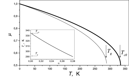
Figure 2: Temperature dependence of the inhomogeneity parameter $\mu$ for different values of the self–action parameter $\alpha$: thick curve relates to $\alpha=0$, thin one — to $\alpha=0.08$ ($T_{c0}=337{\rm K}$). Inset: the temperature of order–disorder transition $T_{c}$ versus the parameter $\alpha$.

The divergency condition $G_{-}^{-1}=0$ of the Green function (54) gives the proper frequency

$$\nu_{0}=\pm\omega-{\rm i}\varpi,\quad\omega\equiv\sqrt{\omega_{0}^{2}-\varpi^{2}}$$ (63)

of the oligomer alternation along the homopolymer chain. Real and imaginary parts are determined by the expressions

$$\begin{split}\omega_{0}\equiv\frac{{\bar{\omega}}_{0}}{\sqrt{\mu(T)}}\left[1+3\alpha\left(1-\frac{9}{8}~{}\frac{T^{2}}{T_{0}^{2}}\right)\right],\\ \varpi\equiv\frac{{\bar{\omega}}_{0}}{\mu(T)}~{}\frac{T_{0}}{T}\left[1+6\alpha\left(1+\frac{3}{8}~{}\frac{T^{2}}{T_{0}^{2}}\right)\right]\end{split}$$ (64)

where the dependence $\mu(T)$ is defined by Eqs. (61), (62); the effective mass in parenthesis after the factor $\alpha\ll 1$ is put to be equal to the value ${\bar{m}}/2$ related to the critical temperature $T_{c}$; characteristic scales of both frequency and temperature are introduced as follows:

$${\bar{\omega}}_{0}\equiv\sqrt{\frac{\tau}{{\bar{m}}}},\quad T_{0}\equiv\frac{\Theta}{2\sqrt{{\bar{m}}\tau}}.$$ (65)

As a result, combination of Eqs.(55), (63) and (64) leads to the final result for the long space period

$$L=2l+\frac{\mu(T)}{\sqrt{\mu(T)-(T_{0}/T)^{2}}}\left[1+\frac{3}{2}\alpha~{}\frac{1+8(T_{0}/T)^{2}+\frac{9}{4}(T_{0}/T)^{-2}}{1-2(T_{0}/T)^{2}}\right]L_{0}$$ (66)

where the characteristic length $L_{0}\equiv D_{0}/{\bar{\omega}}_{0}\sim\sqrt{{\bar{m}}/\tau}~{}\chi^{1/6}b\propto\chi^{1/6}N^{1/2}$ is the function of both parameters $\chi$ and $N$ being thermodynamically independent. Thus, the first of the exponents in the scaling relation $L_{0}\propto\chi^{a}N^{b}$ takes the magnitude $a=1/6$ inherent to the strong segregation regime, whereas the second one ($b=1/2$) is the same for the weak one a . Note that the obtained $\chi$–dependence is caused by the multiplier $\chi^{1/6}$ in the generic relation (55) that is relevant to the former of above regimes, while the method developed addresses to the latter.

V Discussions

The behavior of the system under consideration is controlled by the parameters $\bar{m}$, $\tau$ and $\sigma$ which determine the temperature $T_{c}$ of the order–disorder transition and the long space period $L$ given by Eqs. (62), (66), respectively. Moreover, there is the self–action parameter $0<\alpha\ll 1$ whose value is limited by the magnitude $\alpha_{max}\simeq 0.08$ (see insert in Figure 2). To guarantee positive values of the radicand in Eq. (66) at the critical temperature $T_{c}$, the above parameters have to be constrained by the condition

$$\kappa\geq\sqrt{2}$$ (67)

limiting magnitudes of the principal parameter

$$\kappa\equiv\frac{T_{c}}{T_{0}}=\sqrt{\tau{\bar{m}}}\left(\frac{{\bar{m}}}{\sigma}\right)^{2}(1-2\alpha).$$ (68)

The minimal magnitude of $\kappa$ fixes the choice of the theory parameters according to the condition

$$\sigma\leq 2^{-1/4}{\bar{m}}^{5/4}\tau^{1/4}(1-\alpha).$$ (69)

It would seem from Eqs. (67), (68) that the decrease of the critical temperature $T_{c}$ with passing from the ionically bonded system (such as P4VP–(DBSA)_x) to the hydrogen bonded one (e.g., P4VP–(PDP)_x) is caused only by the growth of the fluctuation parameter $\sigma$ with respect to the mean magnitude of the inhomogeneity parameter $\bar{m}$. It appears, however, that the main reason for such behavior is given by the decrease of the mean–geometrical magnitude $\sqrt{{\bar{m}}\tau}$ of the principal coefficients in the generic Lagrangian (9) (see below).

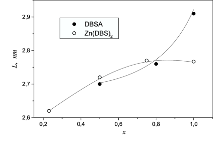
Figure 3: Long space period in the strongly bonded systems as a function of the oligomeric fraction $x$. Solid lines represents the results of fitting in accordance with Eq. (66). Experimental data for P4VP–(DBSA)_x ($\bullet$) and P4VP–(Zn(DBS)₂)_x ($\circ$) at room temperature are taken from Ref. 2 .

Figure 4: Order-disorder transition temperature $T_{c}$ for the weakly bonded system as a function of the oligomeric fraction $x$. The solid line represents the dependence obtained by fitting according to Eq. (62). Experimental data for P4VP–(PDP)_x ($\blacksquare$) are taken from Ref. 8 .

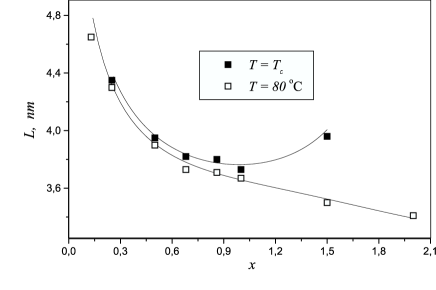
Figure 5: Long space period in the weakly bonded systems as a function of the oligomeric fraction $x$. Solid lines represents the results of fitting in accordance with Eq. (66). Experimental data for P4VP–(PDP)_x at temperature of order–disorder transition $T_{c}$ ($\blacksquare$) and at temperature $T=80^{o}{\rm C}$ ($\square$) are taken from Ref. 8 .

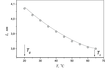
Figure 6: Temperature dependence of the long space period in the weakly bonded system. The solid line represents the dependence obtained by fitting according to Eq. (66). Experimental data for P4VP–(PDP)_x at $x=0.85$ ($\circ$) are taken from Ref. 8 .

To clarify this problem and find explicit form of the dependencies of the temperature of order-disorder transition $T_{c}$ and the period $L$ on the oligomeric fraction $x$, we assume for main theory parameters $\bar{m}$ and $\tau$ the three–parametric relations:

$$\bar{m}=m_{0}+Ax(x_{m}-x),\quad\tau=\tau_{0}+Bx(x_{\tau}-x)$$ (70)

with positive constants $m_{0}$, $\tau_{0}$, $A$, $B$, $x_{m}$, $x_{\tau}$ to be determined. Then, the fitting of the experimental results shown in the Figure 3 in accordance with Eq. (66) where $\tau$, $\bar{m}$ are given by Eq. (70) leads to the following results for the ionically bonded systems:

• the mixtures P4VP–(DBSA)${}_{x}~{}~{}\qquad\qquad\qquad\qquad$

  $$\begin{split}&m_{0}=18,\quad A=8,\quad x_{m}=1.5;\\ &\tau_{0}=0.6,\quad B=1.5,\quad x_{\tau}=1.0;\\ &\alpha=0.01;\quad b=1nm;\quad l=10nm;\end{split}$$ (71)

• the mixtures P4VP–(Zn(DBS)₂)${}_{x}~{}~{}\qquad\qquad\quad\quad$

  $$\begin{split}&m_{0}=5.3,\quad A=26,\quad x_{m}=1.6;\\ &\tau_{0}=0.8,\quad B=0.1,\quad x_{\tau}=1.0;\\ &\alpha=0.01;\quad b=1nm;\quad l=10nm.\end{split}$$ (72)

At $x=1$ one obtains ${\bar{m}}=22$, $\tau=0.6$ for P4VP–(DBSA)_x and ${\bar{m}}=20.9$, $\tau=0.8$ for P4VP–(Zn(DBS)₂)_x. Then, Eq. (68) gives values $\kappa=10^{3}$, $10^{2}$ at $\sigma=1.31$, $4.18$, respectively.

Much more complicated situation occurs in the weakly bonded system P4VP–(PDP)_x. Here, decrease of the parameter (68) results in the narrowing of the temperature domain $T_{0}\div T_{c}$ of the phase separation. All parameters for this class of systems can be determined by the combined fitting of a series of experimental data for the critical temperature $T_{c}$ and the long space period $L$ (see Figures 4 — 6). First constraints follow from the comparison of experimental points for the temperature $T_{c}$ of order–disorder transition (see Figure 4) with fitting results based on Eq. (62) at $\alpha=0.01$, $l=10$ nm:

$$\frac{\Theta m_{0}^{2}}{\sigma^{2}}=562,\quad\frac{A}{m_{0}}=0.155,\quad x_{m}=1.615.$$ (73)

The following of parameters gives application of Eq. (66) for the long space period at the temperature $T=T_{c}$ to the data shown in Figure 5 as the non-monotonous curve:

$$\frac{m_{0}}{\tau_{0}}=1499,\quad\frac{B}{\tau_{0}}=7.968,\quad x_{\tau}=1.926.$$ (74)

Finally, making use of the expression (66) and experimental data for the temperature dependence of the long space period given in Figure 6 yields the last constraint

$$\frac{\Theta}{\sqrt{m_{0}\tau_{0}}}=924.$$ (75)

As a result, taking $m_{0}=1$ at $x=1$ the magnitudes $A=0.155$, $\Theta=23.87$, $\sigma=0.206$ are obtained to provide extremely small value $\tau=5.6\cdot 10^{-3}$ of the hydrogen bonding strength and the temperature scale $T_{0}=160$. At $\alpha=0.01$ this arrives to the rest of parameters $\kappa=2.07$, $\lambda=6.22\cdot 10^{-6}$.

It is worthwhile to discuss separately the dependence of the long space period on the oligomer/monomer ratio at the temperature $T=80^{0}{\rm C}$ that relates to the monotonous decaying curve shown in Figure 5. Because the maximal temperature of the order–disorder transition is $T_{c}\approx 65^{0}{\rm C}$ to be corresponded to $x=0.85$ (see Figure 4), experimental data related to $T=80^{0}{\rm C}$ are obtained for the temperature being beyond of the region of the ordered structure ($T>T_{c}$). From the physical point of view, at the critical temperature $T=T_{c}$ the periodicity of the microphase separated structure formed is caused by long–range correlations, whereas at $T=80^{0}{\rm C}$ only short–range correlations hold to be determined by the homopolymer backbone together with the hydrogen bound surfactant molecules 8 . Fitting of the experimental points for the dependence $L(x)$ at the temperature $T=80^{0}{\rm C}$ can be done on the base of Eq. (66) where one puts $\mu(T)=\mu(T_{c})=1/2$. Then, the values of the parameters obtained differ from those obtained for $T=T_{c}$ by the following constraints:

$$\frac{B}{\tau_{0}}=4.2,\quad x_{\tau}=3.27,\quad\frac{\Theta}{\sqrt{m_{0}\tau_{0}}}=543.$$ (76)

Obviously, this difference is due to the temperature dependence of the hydrogen bonding parameter $\tau$ in the potential energy (4).

To conclude our estimations, we notice the model developed explains successfully a vast variety of peculiarities obtained experimentally for various classes of homopolymer–oligomer mixtures with the interactions of different strength. The resulted data for strong, intermediate and weak coupled systems P4VP–(DBSA)_x, P4VP-(Zn(DBS)₂)_x and P4VP–(PDP)_x, respectively, are given in Table III.

Table 3:

	P4VP–(DBSA)x	P4VP–(Zn(DBS)2)x	P4VP–(PDP)x
$m_{0}$	$18$	$5.3$	$1.000$
$A$	$8$	$26$	$0.155$
$x_{m}$	$1.5$	$1.6$	$1.615$
${\bar{m}}$	$22$	$20.9$	$1.095$
$\tau_{0}$	$0.6$	$0.8$	$6.67\cdot 10^{-4}$
$B$	$1.5$	$0.1$	$5.3\cdot 10^{-3}$
$x_{\tau}$	$1.0$	$1.0$	$1.926$
$\tau$	$0.6$	$0.8$	$5.6\cdot 10^{-3}$
$\sigma$	$1.31$	$4.18$	$0.206$
$\alpha$	$0.01$	$0.01$	$0.01$
$\lambda$	$3.33$	$6.66$	$6.22\cdot 10^{-6}$
$\Theta,{\rm K}$	$10^{3}$	$10^{3}$	$23.87$
$T_{c0},{\rm K}$	$1.41\cdot 10^{5}$	$1.25\cdot 10^{4}$	$337$
$T_{c},{\rm K}$	$1.38\cdot 10^{5}$	$1.22\cdot 10^{4}$	$331$
$T_{0},{\rm K}$	$138$	$122$	$160$
$\kappa$	$10^{3}$	$10^{2}$	$2.07$
$l,{\rm nm}$	$10$	$10$	$10$
$b,{\rm nm}$	$1$	$1$	$1$

It is seen that the coupling weakening arrives to a decrease of both inhomogeneity parameters $\bar{m}$ and $\sigma$, as well as to the crucial decrease of the hydrogen bonding parameter $\tau$ and the self–action parameter $\lambda$, on the one hand, and the characteristic temperatures $T_{c}$ and $\Theta$, on the other hand. According to the relations (68) this leads to extremely large suppression of the value of the parameter $\kappa$ that causes the crucial shrinking the temperature interval of the microphase separation. An analogous effect is caused by the self–action increase.

To get rid of a misunderstanding, we would like to stress a composite character of the approach used. As it is mentioned in Introduction, this circumstance is expressed by dividing the total free energy (1) into two terms, the first one $F_{ho}$ is relevant to the non–associated homopolymer–oligomer mixture, the second one $F_{hb}$ is caused by the hydrogen bonding. These terms are caused by the interactions of principally different physical nature: the behavior of the mixture of non–associated homopolymers and oligomers is determined by the Flory parameter $\chi$, characterizing unfavorable interactions between the the oligomers and the rest of the system; the temperature induced distribution of hydrogen bonds is determined by the parameter $\tau$, giving the strength of this bonding. From the formal point of view, both of the above contributions $F_{ho}(\chi,\phi)$ and $F_{hb}(\tau,x)$ should have a similar dependencies on the state parameters being (apart from the temperature) the volume fraction of the homopolymer $\phi$ for the first contribution, and the oligomer/monomer ratio $x$ for the second one. Because the term $F_{ho}\sim\chi\phi(1-\phi)$ involves the parabolic dependence on the parameter $\phi$ bounded by maximal value $\phi=1$, we took generalized parabolic approximation (70) for the dependence of the hydrogen bonding strength $\tau$ on the oligomer/monomer ratio $x$ which may take values $x>1$.

Apart from the above difference in nature of the interactions, one needs to emphasize at once the difference in the approaches used: the mixture of non–associated homopolymers and oligomers had been studied within the strong segregation limit 2 , whereas for the consideration of the hydrogen bonding we use opposite approach. This difference is kept if the Flory parameter takes large values $\chi\leq 10^{-1}$, whereas the hydrogen bonding strength is relatively small ($\tau\ll 1$). Indeed, the formula (55) for the long space period was obtained within approximation of the sharp interface, which thickness is $\Delta\sim\chi^{-1/2}b\geq 3b$ to be relevant to the strong segregation regime 2 . In the consideration presented, we have focused mainly on the study of the hydrogen bonding on the base of the action (9) that has the form of series in powers of the order parameter $c$ and its derivatives ${\dot{c}}$. Such an expansion supposes making use of the weak segregation limit corresponding to the small values of the parameters $\bar{m}$ and $\tau$.

Finally, it is worthwhile to discuss a difference with an usual picture of the phase transitions that is caused by the self–consistency condition (41). A critical value of the Flory parameter $\chi_{c}$ in usual copolymers is known to be caused by the self–action effects. The accounting of these effects arrives to replacement the bare parameter $\chi$ by the renormalized value $\chi-\chi_{c}$ 19 . However, in our case the value of Flory parameter is so large that the temperature of the separation of non–associated polymer–oligomer mixture is negligible small. As a result, the role of $\chi$ passes to the hydrogen bonding parameter $\tau$ which does not relate to the tendency of monomers of the different kinds to avoid each other. However, as it is shown by the considerations given in 26 , 27 , understanding of the whole picture of microphase separation, including the temperature dependence of the structure period, demands accounting the inhomogeneity in the distribution of oligomers along homopolymer chains. Within the approach developed, this is reached by means of the effective kinetic energy (6), with the mass fluctuating due to the temperature dependence of hydrogen bonding. This dependence leads to the reduction (42) of the effective mass $m_{ef}$ that causes a phase transition from stochastic to periodic distribution of the oligomers along the homopolymer chain. However, if the critical point is fixed usually by the condition $m_{ef}=0$ 10 , in our case the critical temperature $T_{c}$ relates to the finite magnitude $m_{ef}={\bar{m}}/2$ of the effective mass which has a singularity ${\rm d}m_{ef}/{\rm d}T=-\infty$ in the temperature derivative (see Figure 2).

Appendix A Derivation of a generic relation for microphase structure period

Following 2 we suppose the period of the microphase structure to be determined by the minimum of the specific free energy

$$f\equiv\frac{1}{V}\frac{F_{int}+F_{str}}{T};\quad V\equiv LS,\quad L\equiv 2l+D$$ (77)

related to the first term in Eq. (1). Being the free energy of the homopolymer–oligomer mixture, this term consists of the interfacial and stretching components $F_{int}$, $F_{str}$ measured in the temperature units $T$ per the domain volume $V$ (according to Figure 1 $L$, $l$ and $D$ are the long space period, the length of the oligomer tail and the thickness of the homopolymer layer, respectively; $S$ is the domain surface area).

The interfacial free energy is stipulated by the loss of conformational entropy caused by the localization of the homopolymer chains within the interface of thickness $\Delta$. Due to unfavorable interaction $\chi$ between the oligomer tails and the polymer layer the chains form up loops containing segments of number $\mathcal{N}_{s}\sim\chi^{-1}$ Helfand1971 . Then, within the model of the random walk, the interface thickness is estimated by the relations $\Delta^{2}\simeq\mathcal{N}_{s}b^{2}\sim b^{2}/\chi$ where $b$ is the segment length. Respectively, the interfacial free energy $F_{int}\simeq\mathcal{N}_{l}~{}T$ is determined by the number $\mathcal{N}_{l}\simeq S\Delta/\mathcal{N}_{s}b^{3}$ of the loops within the interface. As a result, we obtain the estimation

$$F_{int}\sim\frac{\chi^{1/2}}{b^{2}}T~{}S.$$ (78)

Another addition $F_{str}$ is caused by the stretching of the surfactant side chains, whereas the stretching of the homopolymer chains enlarges only the volume part of the free energy. This addition is expressed by the simple equality $F_{str}\simeq\mathcal{N}_{c}n_{s}F_{1}$ where the first factor $\mathcal{N}_{c}\simeq DS/Nb^{3}$ gives the number of chains per layer, the second multiplier $n_{s}\simeq(b/\lambda)N$ is the number of the oligomer molecules per chain of $N$ segments ($\lambda$ is period of the oligomers alternating along the chain) and the last factor $F_{1}\sim(l^{2}/nb^{2})T$ presents the free energy of stretching a side chain of $n$ segments to a length $l$. Combining the above multipliers, we find the estimation for the total free energy of stretching

$$F_{str}\sim\frac{l^{2}DS}{nb^{4}\lambda}~{}T.$$ (79)

To derive the explicit expression for the dependence of the free energy (77) on the layer thickness $D$ we need to use an obvious condition $2lS\equiv\mathcal{N}_{c}n_{s}v_{s}$ where $v_{s}=nb^{3}$ is the volume of surfactant molecule. As a result, we obtain the relation

$$\frac{2l}{D}\equiv\frac{b}{\lambda}~{}n,$$ (80)

according to which the period $\lambda$ defines the rest of geometrical characteristics of the microphase separated structure. Inserting Eqs. (78) — (80) into Eq. (77), we arrive to the final expression for the interfacial free energy:

$$f\sim\frac{\frac{\chi^{1/2}}{D}+\frac{n}{\lambda^{3}}D^{2}}{\left[1+(b/\lambda)n\right]b^{2}}$$ (81)

where numerical coefficients are dropped. The minimization condition ${\partial f}/{\partial D}=0$ arrives at the steady–state values of the homopolymer layer thickness and the oligomer length

$$D\sim\frac{\chi^{1/6}}{n^{1/3}}\lambda,\quad 2l\sim\left(\chi^{1/6}n^{2/3}\right)b.$$ (82)

It is convenient to express above results by means of the dimensionless frequency of the oligomer alternating along the homopolymer chain:

$$\omega\equiv\frac{2\pi}{\lambda/b}=\omega_{max}X;\quad\omega_{max}\equiv 2\pi,~{}~{}X\equiv\frac{b}{\lambda}$$ (83)

where $X$ is the averaged oligomeric fraction per homopolymer. So, the long space period of the microphase separated structure takes the form

$$L\equiv 2l+D\simeq\chi^{1/6}n^{-1/3}\left(n+\frac{2\pi}{\omega}\right)b.$$ (84)

Appendix B Calculations of convolution integrals

Self–energy functions

Calculations of the self–energy functions (47), (48) lead to a rather tedious procedure due to the convolution integrals. To demonstrate the line of these calculations we consider in details the simplest integral related to the first term in Eq. (48):

$$\Sigma_{-}^{\mu}(\nu)=\mu^{2}\int\frac{{\rm d}\nu_{1}}{2\pi}S(\nu_{1})G_{-}(\nu-\nu_{1}).$$ (85)

Making use of the expressions (34) for the structure factor $S$ and Green function $G_{-}$, where the frequency dispersed parameter $\tau(\nu)$ is replaced by its bare magnitude $\tau$, arrives at the convolution integral

$$\Sigma^{\mu}_{-}(\nu)=\frac{\mu^{2}}{2\pi n_{c}^{3}}\int\frac{{\rm d}\nu_{1}}{(\omega_{s}^{2}+\nu_{1}^{2})\left[\omega_{s}-{\rm i}(\nu-\nu_{1})\right]}$$ (86)

where a characteristic frequency $\omega_{s}\equiv\tau/n_{c}$ is introduced. This integral has the poles $\pm{\rm i}\omega_{s}$ and $\nu+{\rm i}\omega_{s}$ (see Figure 7a).

Figure 7: Poles of the convolution integral in Eqs. (86) (a) and (91) (b). $\delta\equiv\sqrt{\xi_{2}^{2}-\xi_{1}^{2}}$.

In accordance with the theory of residues book poles , the integral in Eq. (86) is reduced to sum over two of these residues that locate in upper half–plane of the complex frequency $\nu_{1}$:

$$2\pi{\rm i}\left[\frac{-\rm{i}}{2{\rm i}\omega_{s}\cdot(-\nu)}+\frac{-\rm{i}}{\nu\cdot(\nu+2{\rm i}\omega_{s})}\right]$$ (87)

where terms in the square brackets relate to the poles ${\rm i}\omega_{s}$ and $\nu+{\rm i}\omega_{s}$, respectively. After a simple algebra this expression yields

$$\Sigma_{-}^{\mu}=\frac{\mu^{2}}{\tau^{2}n_{c}}~{}\frac{1+\frac{\rm{i}}{2}\xi}{4+\xi^{2}},\quad\xi\equiv\frac{\nu}{\omega_{s}}.$$ (88)

Analogously, the rest of convolution integrals is calculated giving final form of Eqs.(47), (48):

$$\Sigma=\frac{\mu^{2}}{2\tau^{3}n_{c}}~{}\frac{1}{4+\xi^{2}}+\frac{\lambda^{2}}{8\tau^{4}n_{c}^{2}}~{}\frac{1}{9+\xi^{2}},$$ (89)

$$\Sigma_{\pm}=\frac{\mu^{2}}{\tau^{2}n_{c}}~{}\frac{1\mp{{\rm i}\over 2}\xi}{4+\xi^{2}}+\frac{\lambda^{2}}{8\tau^{3}n_{c}^{2}}~{}\frac{3\mp{\rm i}\xi}{9+\xi^{2}}.$$ (90)

Renormalization mass parameter

Explicit form of the renormalization mass parameter (41) is determined by the structure factor (52) and Green function (54) with the effective mass (42) and parameter $\tau(\nu)$ being replaced by bare $\tau$:

$$\Delta=\frac{\sigma^{2}}{\pi n_{c}m_{ef}}\int\frac{(\xi_{1}-\xi_{0}^{-1}\xi^{2})\xi^{2}{\rm d}\xi}{(\xi^{2}-2{\rm i}\xi_{1}\xi-\xi_{2}^{2})(\xi^{2}+2{\rm i}\xi_{1}\xi-\xi_{2}^{2})}$$ (91)

where one denotes

$$\begin{split}\xi_{0}\equiv&\frac{16m_{ef}\tau}{n_{c}}\left(\frac{\mu^{2}}{4}+\frac{\lambda^{2}}{3^{4}\tau n_{c}}\right)^{-1},\\ \xi_{1}\equiv&\frac{n_{c}^{2}}{2m_{ef}\tau}\left[1+\frac{1}{8\tau^{3}n_{c}}\left(\mu^{2}+\frac{\lambda^{2}}{9\tau n_{c}}\right)\right],\\ \xi_{2}^{2}\equiv&\frac{n_{c}^{2}}{m_{ef}\tau}\left[1-\frac{1}{4\tau^{3}n_{c}}\left(\mu^{2}+\frac{\lambda^{2}}{6\tau n_{c}}\right)\right].\end{split}$$ (92)

The integral in Eq. (91) has the pole structure that is shown in Figure 7b. As above, the sum over residues located in the upper half–plane of the complex frequency $\xi$ yields the integral value

$$\frac{\pi}{2}\left(1-\frac{\xi_{2}^{2}-4\xi_{1}^{2}}{\xi_{0}\xi_{1}}\right).$$ (93)

With accounting the notices (92) and keeping only the terms of the second order of smallness over parameters $\mu$ and $\lambda$, one obtains the final expression (56).

References

- (1) M. Antonietti, A. Wenzel, A. Thunemann, Langmuir 12, 2111 (1996)
- (2) O. Ikkala, J. Ruokolainen, G. Ten Brinke, M. Torkkeli and R. Serimaa, Macromolecules 28, 7088, 7779 (1995).
- (3) J. Ruokolainen, G. Ten Brinke, O. T. Ikkala, M. Torkkeli and R. Serimaa, Macromolecules 29, 3409 (1996).
- (4) J. Ruokolainen et al., Phys. Rev. E54, 6646 (1996).
- (5) G. Ten Brinke, J. Ruokolainen and O. Ikkala, Europhys. Lett., 35 (2), 91 (1996).
- (6) F. Tanaka, M. Ishida, Macromolecules 30, 1836 (1997)
- (7) E. Dormidontova, G. Ten Brinke, Macromolecules 31, 2649 (1998)
- (8) L. Leibler, Macromolecules 13, 1602 (1980)
- (9) G. N. Fredrickson, S. T. Milner, L. Leibler, Macromolecules 25, 6341 (1992)
- (10) C. D. Sfatos, E. I. Shakhnovich, Phys. Rep. 288, 77 (1997).
- (11) J. Zinn-Justin, Quantum Field Theory and Critical Phenomena (Clarendon Press, Oxford, 1993).
- (12) A. I. Olemskoi, Physica A270, 444 (1999).
- (13) A. I. Olemskoi, V.A.Brazhnyi, Physica A273, 368 (1999).
- (14) A. I. Olemskoi,Physics–Uspekhi 171 503 (2001).
- (15) T. A. Vilgis, J. Phys. A 24, 5321 (1991)
- (16) P. C. Martin, E. D. Siggia, H. A. Rose, Phys. Rev. A 8, 423 (1973).
- (17) J. Kurchan, J. Phys. (France) I, 2, 1333 (1992).
- (18) E. Helfand, Y. Tagani, J. Polymer Sci. B 9, 799 (1971)
- (19) K. R. Shull, Macromolecules 25, 2122 (1992).
- (20) R. Remmert, Theory of Complex Functions (Springer, New York, 1991)