Direct extraction of the Eliashberg function for electron-phonon coupling: A case study of Be(10$\mathbf{\bar{1}}$0)

Abstract

We propose a systematic procedure to directly extract the Eliashberg function for electron-phonon coupling from high-resolution angle-resolved photoemission measurement. The procedure is successfully applied to the Be(10$\bar{1}$0) surface, providing new insights to electron-phonon coupling at this surface. The method is shown to be robust against imperfections in experimental data and suitable for wider applications.

Electron-phonon coupling (EPC) is the basis for many interesting phenomena in condensed matter physics such as conventional superconductivity. Its possible role in the high-$T_{c}$ cuprates is also being actively discussed Darmascelli2003 ; Egami2002 ; Lanzara2001 . Experimentally, recent advances in high-resolution (both energy and momentum) angle-resolved photoemission spectroscopy (ARPES) have stimulated many studies on EPC in various systems Lanzara2001 ; Matzdorf1996 ; Balasubramanian1998 ; Hengsberger1999 ; Valla1999 ; Lashell2000 ; Rotenberg2000 ; Tang2002 ; Luh2002 ; Ast2002 . These ARPES measurements usually yield the mass enhancement factor $\lambda$ Grimvall , which characterizes the strength of EPC, along with some primitive information about its spectral structure such as the dominant phonon mode. It is highly desirable to take advantage of these high-resolution data and obtain full characteristics of EPC.

Theoretically, the full characteristics of EPC are described by the Eliashberg function $\alpha^{2}F(\omega;\epsilon,\mathbf{\hat{k}})$ Grimvall , the total transition probability of a quasi-particle from/to the state $(\epsilon,\mathbf{\hat{k}})$ by coupling to boson (phonon) modes of frequency $\omega$ Eiguren2002 . Essentially all physical quantities related to EPC can be deduced from the function. For instance, the mass enhancement factor $\lambda$ is related to the Eliashberg function by Grimvall ,

$$\lambda=2\int_{0}^{\infty}\frac{d\omega}{\omega}\alpha^{2}F(\omega;\epsilon_{F},\hat{\mathbf{k}})\,.$$ (1)

In this Letter, we present a systematic procedure to directly extract the Eliashberg function from the high-resolution ARPES data. The Maximum Entropy Method (MEM) Gubernatis1991 is employed to overcome the numerical instability inherent to such efforts Verga2003 . With Eq.1, our procedure also gives a reliable estimate of the mass enhancement factor $\lambda$, without making ad hoc assumptions on phonon model or requiring low temperature measurement Ast2002 ; Balasubramanian1998 ; Hengsberger1999 ; Lashell2000 ; Tang2002 ; Rotenberg2000 ; Valla1999 ; Luh2002 .

This procedure is illustrated using new high-resolution ARPES data at the Be(10$\bar{1}$0) surface. This system is ideal for testing the new procedure because Be has a broad phonon band ($\sim 80\,\mathrm{meV}$), thereby removing the need for super-high-energy resolution. Also, results of measurements Tang2002 ; Hofmann1997 and theoretical calculations Lazzeri2000 for this surface have been published, providing references for comparison.

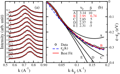
Figure 1: (Color online) (a) Momentum distribution curves (MDCs) of S1 surface state of Be(10$\bar{1}$0) along $\bar{\mathrm{A}}\bar{\Gamma}$. The numbers denote the initial state energies in meV. The solid lines show the Lorentzian fittings. (b) Quasi-particle dispersion determined from the MDCs (circles). The solid lines show fittings to the dispersion with the procedure detailed in the text using different bare quasi-particle dispersions $\epsilon_{0}(\mathbf{k})$. The parameters $\upsilon_{F}$ ($\mathrm{eV}\cdot\mathrm{\AA}/\hbar$) and $\beta$ ($\mathrm{eV}\cdot\mathrm{\AA}^{2})$ of $\epsilon_{0}(\mathbf{k})$ are shown in the inset. The dashed line indicates $\epsilon_{0}(\mathbf{k})$ that results in the best fit.

The photoemission experiments were performed at the Advanced Light Source (ALS) on Beamline 10.0.1 using a display high-resolution Scienta 2002 energy analyzer at 24  eV photon energy with total energy resolution $10\,\mathrm{meV}$ and angular resolution $\pm 0.15^{\circ}$ in $6\times 10^{-11}$ Torr vacuum and at $T=30\,\mathrm{K}$. The cleaning procedure for the Be(10$\bar{1}$0) sample was described earlier Balasubramanian1998 .

Figure 1(a) shows the momentum distribution curves (MDCs) of the Be(10$\bar{1}$0) S1 surface state. The quasi-particle dispersion $\epsilon(\mathbf{k})$ is determined from MDCs by Lorentzian fittings Lashell2000 , and is shown in Fig. 1(b). The real part of the self energy is calculated by $\mathrm{Re}\Sigma(\epsilon,\hat{\mathbf{k}})=\epsilon(\mathbf{k})-\epsilon_{0}(\mathbf{k})$, where $\epsilon_{0}(\mathbf{k})$ is the bare quasi-particle dispersion, i.e., without EPC. Within the small energy scale considered, it is sufficient to approximate $\epsilon_{0}(\mathbf{k})\approx-\hbar\upsilon_{F}(k-k_{F})+\beta(k-k_{F})^{2}$. Following the extrapolation procedure that will be detailed later, we find that $\hbar\upsilon_{F}=2.95\,\mathrm{eV}\cdot\mathrm{\AA}$ and $\beta=6.74\,\mathrm{eV}\cdot\mathrm{\AA}^{2}$ provide the best fit to the data, as shown in Fig. 1(b). The resulting real part of the self energy for the S1 state is shown in Fig. 2(a).

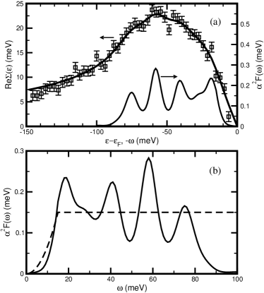
Figure 2: (a) Real part of the self energy. Solid line shows the MEM fitting. The error bars $\sigma_{i}=1\,\mathrm{meV}$ are determined from the noise level of the data. (b) Extracted Eliashberg function. The dashed line shows the constraint function $m(\omega)$ used: $\omega_{D}=15\,\mathrm{meV}$, $\omega_{m}=100\,\mathrm{meV}$, and $m_{0}=0.15$ (See Eq. 6). The extracted Eliashberg function is also shown in (a) to indicate the origin of its structures in the self-energy (note the x-axis is reversed).

The real part of the self energy is related to the Eliashberg function by Grimvall :

$$\mathrm{Re}\Sigma(\epsilon,\mathbf{\hat{k}};T)=\int_{0}^{\infty}d\omega\alpha^{2}F(\omega;\epsilon,\mathbf{\hat{k}})K\left(\frac{\epsilon}{kT},\frac{\omega}{kT}\right)\,,$$ (2)

where $K(y,y^{\prime})=\int_{-\infty}^{\infty}dxf(x-y)2y^{\prime}/(x^{2}-y^{\prime 2})$ with $f(x)$ being the Fermi distribution function. Eq. 2 is valid for a normal Fermi liquid coupled with boson field(s). For a normal metal that has no sharp electronic structure around the Fermi surface within the small energy scale of the order of the phonon bandwidth (80 meV), dependence on the initial state energy $\epsilon$ can be ignored because $d\alpha^{2}F(\omega;\epsilon,\hat{\mathbf{k}})/d\omega\gg d\alpha^{2}F(\omega;\epsilon,\hat{\mathbf{k}})/d\epsilon$ Grimvall . Thus, $\alpha^{2}F(\omega;\epsilon,\hat{\mathbf{k}})$ in Eq. 2 can be replaced by the Eliashberg function at the Fermi level $\alpha^{2}F(\omega)$, defined as $\alpha^{2}F(\omega)\equiv\alpha^{2}F(\omega;\epsilon_{F},\hat{\mathbf{k}})$.

With this simplification, Eq. 2 poses an integral inversion problem for extracting $\alpha^{2}F(\omega)$ from the real part of the self energy. The most straightforward way to do the inversion is the least-squares method that minimizes the functional:

$$\chi^{2}=\sum_{i=1}^{N_{D}}\frac{\left[D_{i}-\mathrm{Re}\Sigma(\epsilon_{i})\right]^{2}}{\sigma_{i}^{2}}\,,$$ (3)

against the Eliashberg function $\alpha^{2}F(\omega)$, where $D_{i}$ are the data for the real part of the self energy at energy $\epsilon_{i}$; $\mathrm{Re}\Sigma(\epsilon_{i})$ is defined by Eq. 2 and is a functional of $\alpha^{2}F(\omega)$; $\sigma_{i}$ are the error bars of the data; and $N_{D}$ is the total number of data points. Unfortunately, such a straightforward approach fails because the inversion problem defined by Eq. 2 is unstable mathematically and the direct inversion tends to exponentially amplify the high-frequency data noise, resulting in unphysical fluctuations and negative values in the extracted Eliashberg function.

To overcome the numerical instability in the direct inversion, one needs to incorporate the physical constraints into the fitting process. The most important constraint is that the Eliashberg function must be positive. To do this, we employ the Maximum Entropy Method (MEM) Gubernatis1991 , which minimizes the functional:

$$L=\frac{\chi^{2}}{2}-aS\,$$ (4)

where $\chi^{2}$ is defined in Eq. 3, and $S$ is the generalized Shannon-Jaynes entropy,

$$S=\int_{0}^{\infty}d\omega\left[\alpha^{2}F(\omega)-m(\omega)-\alpha^{2}F(\omega)\ln\frac{\alpha^{2}F(\omega)}{m(\omega)}\right]\,.$$ (5)

The entropy term imposes physical constraints to the fitting and is maximized when $\alpha^{2}F(\omega)=m(\omega)$, where $m(\omega)$ is the constraint function and should reflect our best a-priori knowledge for the Eliashberg function of the specific system. In this study, we use the following generic form:

$$m(\omega)=\left\{\begin{array}[]{ll}m_{0}\left(\omega/\omega_{D}\right)^{2}\,,&\omega\leq\omega_{D}\\ m_{0}\,,&\omega_{D}<\omega\leq\omega_{m}\\ 0\,,&\omega>\omega_{m}\end{array}\right.\,,$$ (6)

which encodes the basic physical constraints of the Eliashberg function: (a) it is positive; (b) it vanishes at the limit $\omega\rightarrow 0$; (c) it vanishes above the maximal phonon frequency.

The multiplier $a$ in Eq. 4 is a determinative parameter that controls how close the fitting should follow the data while not violating the physical constraints. When $a$ is small, the fitting will follow the data as closely as possible, and when $a$ is large, the extracted Eliashberg function will not deviate much from $m(\omega)$. There exist a number of schemes (eg. historic, classic, Bryan’s method, etc.) that choose the optimal value of $a$ based on the data and the constraint function $m(\omega)$ Gubernatis1991 . In this study, the classic method is used.

To minimize Eq. 4, Eqs. 2 and 5 are discretized using the iterated trapezoid rule for the integral over $\omega$, and $\alpha^{2}F(\omega)$ is optimized using a Newton algorithm developed by Skilling and collaborators that searches along three prescribed directions in each iterative step Gubernatis1991 . Detailed reviews of the algorithms can be found in Ref. Gubernatis1991, .

Figure 2(b) shows the extracted Eliashberg function of the Be(10$\bar{1}$0) S1 surface state and the constraint function $m(\omega)$. It resolves a number of peaks approximately at 40, 60, and 75 meV. Low energy modes with $\omega<30\,\mathrm{meV}$ are also evident. When compared with the first-principles calculations of the phonon dispersion of this system Lazzeri2000 , the resolved peaks correspond well to those surface phonon modes. The extracted Eliashberg function automatically cuts off at $\sim 80\,\mathrm{meV}$, which is also consistent with the calculation Lazzeri2000 . The mass enhancement factor $\lambda$ is calculated by Eq. 1, yielding a value $0.68\pm 0.08$, consistent with $\lambda=0.65$ obtained in previous measurements using temperature-dependent line shapes Tang2002 .

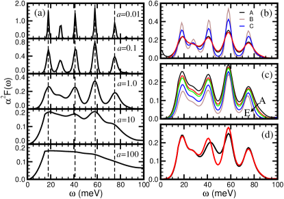
Figure 3: Various robustness tests to the fittings. The red line in each figure indicates the nominal result as presented in Fig. 2(b). (a) Extracted Eliashberg functions for different values of $a$. (b) Extracted Eliashberg functions for different constraint function parameters. For each curve, one of parameters used in Fig. 2(b) is changed: A. $\omega_{D}\Rightarrow 0$; B. $\omega_{m}\Rightarrow 200\,\mathrm{meV}$; C. $m_{0}\Rightarrow 0.3$. The corresponding values of $a$ determined by the classic method are: A. $a=1.13;$ B. $a=0.22$; C. $a=0.43$. The nominal result has $a=1.44$. (c) Extracted Eliashberg functions of the fittings A–E shown in Fig. 1(b) for different bare particle dispersions. (d) Extracted Eliashberg function (black line) after dropping the abnormal data point at $\sim 47\,\mathrm{meV}$ in Fig. 2(a).

We have carried out systematic tests to assess the effects of various parameters involved in the fitting and the robustness of the procedure against data imperfections. These tests are summarized in Fig. 3. Based on these tests, which will be detailed below, we conclude that the fitting procedure can be well controlled to provide reliable physical insights.

The most important fitting parameter is the multiplier $a$. Figure 3(a) shows the fitting results as a function of $a$. Changing the value of $a$ does not change qualitative features of the extracted Eliashberg function such as the number and the positions of the peaks, although the quantitative changes of the “contrast” are evident. Furthermore, the estimate of $\lambda$ is not sensitive to the value of $a$: for $a$ changing from $0.01$ to $100$, $\lambda$ varies only between $0.64$ and $0.69$.

The classic method determines the optimal value of $a$ based on the data and the constraint function. Inevitably, the parameters $m_{0}$, $\omega_{R}$, and $\omega_{m}$ in the constraint function influence the decision of classic method, as demonstrated in Fig. 3(b). A proper choice of these parameters is important to ensure that the algorithm makes the correct decision. In Fig. 2(b), $m_{0}$ is roughly the average height of the Eliashberg function, $\omega_{m}$ is slightly higher than the maximal phonon frequency, and a small but nonzero value of $\omega_{D}$ is chosen to suppress the artifact near the zero frequency as seen in in Fig. 3(b) for $\omega_{D}=0$. In this way, we have a constraint function that is close enough to the real Eliashberg function and is still sufficiently structureless for an unbiased fitting.

The parameters in the bare particle dispersion, $\upsilon_{F}$ and $\beta$, are determined from extrapolation to the higher initial state energy. $\upsilon_{F}$ and $\beta$ are inter-dependent because given a value of $\beta$, there is only one value of $\upsilon_{F}$ (within a small window) that can yield the real part of the self energy which has the correct asymptotic behavior and can be fitted by Eq. 2. To find the optimal bare quasi-particle dispersion, we tried a number pairs of ($\upsilon_{F}$, $\beta$) to generate the real part of the self energy, then ran the MEM fitting within $\epsilon<150\,\mathrm{meV}$. The optimal pair of ($\upsilon_{F}$, $\beta$) is the one that provides the best fit to the dispersion data in the larger energy window (300 meV). This procedure is demonstrated in Fig. 1(b). The corresponding extracted Eliashberg functions for different values of ($\upsilon_{F}$, $\beta$) are shown in Fig. 3(c). It can be seen that fittings with less optimal values of ($\upsilon_{F}$, $\beta$) yield result rather close to the nominal one. This removes the need for high accuracy in determining the bare quasi-particle dispersion.

The MEM fitting is rather robust against the data imperfections such as accidental data anomaly, as demonstrated in Fig. 3(d). The robustness has two origins: (a) physical constraints built in the fitting automatically filter out those unphysical data fluctuations; (b) although one data point may be anomalous, it is statistically less likely that a number of data points become anomalous simultaneously in a coherent way.

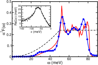
Figure 4: (Color online) A test to the data extraction procedure. Solid line shows the pre-defined Eliashberg function. The filled circle-line shows the extracted Eliashberg function. Dashed line shows $m(\omega)$ with parameters $\omega_{D}=50\,\mathrm{meV}$, $\omega_{m}=100\,\mathrm{meV}$, and $m_{0}=0.2$4. Inset shows the data presented to the program and the MEM fitting. Gaussian noise with $\sigma_{i}=1\,\mathrm{meV}$ has been added to the self-energy data. $T=30\,\mathrm{K}$.

Figure 4 provides a further test on the robustness of the MEM fitting. Here, we generate a set of data of the real part of the self energy from a pre-defined Eliashberg function. Gaussian noise is added to simulate the realistic experimental situation. Figure 4 shows a typical result of the test. It can be seen that the MEM successfully extracts the overall qualitative features of the predefined Eliashberg function although the data are rather noisy. The mass enhancement factor calculated from Eq. 1 is $0.35\pm 0.05$, which is very close to the exact value $0.35$.

Our MEM fitting scheme can be further improved by using a better constraint function $m(\omega)$. For instance, if the phonon density of states $F(\omega)$ is known from other reliable sources, one can use $m(\omega)=\alpha_{0}^{2}\times F(\omega)$ with $\alpha_{0}^{2}$ being determined by optimizing its posterior probability Gubernatis1991 . Such a scheme should allow a seamless integration of the existing knowledge of the fine spectral structure and the newly extracted coupling strengths.

Our systematic procedure to extract the Eliashberg function has a number of advantages. (a) ARPES has much wider applicability than the traditional method using the single-particle tunneling characteristics Grimvall . (b) ARPES allows measurements along different directions, so the Eliashberg function $\alpha^{2}F(\omega;\epsilon,\hat{\mathbf{k}})$ on the whole Fermi surface could be determined. (c) Equation 2, the theoretical basis of our method, makes only minimal assumption on the nature of the system, i.e., a normal Fermi liquid without strong electronic structure near the Fermi energy. (d) The procedure only utilizes the data for $\mathrm{Re}\Sigma(\epsilon)$, which is easier to determine and less prone to the imperfections than $\mathrm{Im}\Sigma(\epsilon)$.

Here, our case study also provides new insights to EPC at the Be(10$\bar{1}$0) surface. (a) The extracted Eliashberg function is significantly different from the simple fictitious models (e.g., Debye and Einstein models) previously used to interpret the data Lashell2000 ; Tang2002 ; (b) More than 75% (0.5 out of 0.68) of the enhanced $\lambda$ is contributed by the low frequency surface modes below $50\,\mathrm{meV}$ that are not present in the bulk phonon spectrum. Similar behavior is also observed in Be(0001) surface Eiguren2002 ; Tang2003 . This raises the question whether the low frequency surface phonon modes are responsible for the large mass enhancement factors observed in many metal surfaces Matzdorf1996 ; Balasubramanian1998 ; Hengsberger1999 ; Valla1999 ; Lashell2000 ; Rotenberg2000 ; Tang2002 ; Ast2002 ; (c) The average phonon frequency Kulic2000 , $\ln\omega_{\log}=(2/\lambda)\int_{0}^{\infty}d\omega[\alpha^{2}F(\omega)/\omega]\ln\omega,$ is calculated to be $29\,\mathrm{meV}$, which is substantially smaller than its bulk value ($\sim 60\,\mathrm{meV}$) Balasubramanian1998 . This reduces the estimated $T_{c}$ for possible superconductivity.

In summary, we have proposed a systematic way to extract the Eliashberg function from the high-resolution ARPES data. The MEM is employed to overcome the data imperfections and numerical instability. By using this new technique, we have provided new insights to EPC at the Be(10$\bar{1}0)$ surface. We expect the technique to be useful in many situations, for instance, in the study of the possible role of EPC in high-temperature superconductivity.

- (1) A. Damascelli, Z. Hussain, and Z.-X. Shen, Rev. Mod. Phys. 75, 473 (2003).
- (2) T. Egami, J. Supercond. 15, 373 (2002); T. Egami and P. Piekarz, Solid State Commun. (2003) (in press).
- (3) A. Lanzara, P.V. Bogdanov, X.J. Zhou, S.A. Kellar, D.L. Feng, E.D. Lu, T. Yoshida, H. Eisaki, A. Fujimori, K. Kishio, J.-I. Shimoyama, T. Noda, S. Uchida, Z. Hussain, Z.-X. Shen, Nature, 412, 510 (2001).
- (4) R. Matzdorf, G. Meister, A. Goldmann, Phys. Rev. B 54, 14807 (1996).
- (5) T. Balasubramanian, E. Jensen, X.L. Wu and S.L. Hulbert, Phys. Rev. B 57, R6866 (1998).
- (6) M. Hengsberger et al., Phys. Rev. Lett. 83, 592 (1999); M. Hengsberger, R. Fresard, D. Purdie, P. Segovia, and Y. Baer, Phys. Rev. B 60, 10796 (1999).
- (7) T. Valla, A.V. Fedorov, P.D. Johnson, S.L. Hulbert, Phys. Rev. Lett. 83, 2085 (1999).
- (8) S. LaShell, E. Jensen, and T. Balasubramanian, Phys. Rev. B 61, 2371(2000).
- (9) E. Rotenberg, J. Schaefer, S.D. Kevan, Phys. Rev. Lett. 84, 2925 (2000).
- (10) S.-J. Tang, Ismail, P. T. Sprunger, and E. W. Plummer, Phys. Rev. B 65, 235428 (2002).
- (11) C.R. Ast and H. Höchst, Phys. Rev. B 66, 125103 (2002).
- (12) D.-A. Luh, T. Miller, J. J. Paggel, T.-C. Chiang, Phys. Rev. Lett. 88, 256802 (2002).
- (13) G. Grimvall, The Electron-Phonon Interaction in Metals, edited by E. Wohlfarth (North-Holland, New York, 1981).
- (14) A. Eiguren, B. Hellsing, F. Reinert, G. Nicolay, E.V. Chulkov, V.M. Silkin, S. Hüfner, P.M. Echenique, Phys. Rev. Lett. 88, 066805 (2002); A. Eiguren, S. de Gironcoli, E.V. Chulkov, P.M. Echenique, E. Tosatti, Phys. Rev. Lett. 91, 166803 (2003).
- (15) See, for instance, J.E. Gubernatis, M. Jarrell, R.N. Silver, D.S. Sivia, Phys. Rev. B 44, 6011 (1991) and references therein; M. Jarrell, J.E. Gubernatis, Phys. Rep. 269, 133 (1996); M. Jarrell, preprint, http://www.physics.uc.edu/~jarrell/PAPERS/MEM_AdvPhys.pdf.
- (16) S. Verga, A. Knigavko, F. Marsiglio, Phys. Rev. B 67, 054503 (2003).
- (17) Ph. Hofmann, E.W. Plummer, Surf. Sci. 377, L330 (1997).
- (18) M. Lazzeri, S. de Gironcoli, Surf. Sci. 454-456, 442 (2000).
- (19) M.L. Kulić, Phys. Rep. 338, 1 (2000).
- (20) S.-J. Tang et al., Physica Status Solidi, to be published.