Full Counting Statistics of Multiple Andreev Reflections

Abstract

We derive the full distribution of transmitted particles through a superconducting point contact of arbitrary transparency under voltage bias. The charge transport is dominated by multiple Andreev reflections. The counting statistics is a multinomial distribution of processes, in which multiple charges $ne$ ($n=1,2,3,\ldots$) are transferred through the contact. For zero temperature we obtain analytical expressions for the probabilities of the multiple Andreev reflections. The current, shot noise and high current cumulants in a variety of situations can be obtained from our result.

The complete understanding of the electronic transport in mesoscopic systems requires information that goes beyond the analysis of the current. This explains the great attention devoted in the last years to current fluctuations in these systems Blanter2000 . An important goal is to obtain the full current distribution. This was realized by Levitov and coworkers Levitov1993 , who borrowed the concept of full counting statistics (FCS) for photons and adapted it to electrons in mesoscopic systems. FCS gives the probability $P(N)$ that $N$ charge carriers pass through a conductor in the measuring time. From the knowledge of these probabilities one can easily derived not only the conductance and noise, but all the cumulants of the current distribution. Since the introduction of FCS for electronic systems, the theory has been sophisticated and applied to many different contexts (see a recent review, nazarov:03 ). In particular one of the authors and Nazarov have shown that, based on a Keldysh-Green’s function method, one can calculate in a unified manner the FCS of all contacts involving superconducting elements Belzig2001 .

In the context of superconductivity the basic situation, in which the FCS has not been yet investigated, is a point contact between two superconductors out of equilibrium. In this system the transport properties for voltages $V$ below the superconducting gap $\Delta$ are dominated by coherent multiple Andreev reflections (MAR) Klapwijk1982 . In these processes a quasiparticle undergoes a cascade of Andreev reflections until it reaches an empty state in one of the leads. Recently, the microscopic theory of MAR Bratus1995 has provided a new insight into this problem and has allowed the calculation of properties beyond the current such as the shot noise Cuevas1999 . The predictions of this theory have been quantitatively tested in an impressive series of experiments in atomic-size contacts Scheer1997 ; Scheer1998 ; Cron2001 . In particular, the analysis of the shot noise Cuevas1999 ; Cron2001 has suggested, that the current at subgap energies proceeds in “giant” shots, with an effective charge $q\sim e(1+2\Delta/|eV|)$. However, strictly speaking, the question of whether the charge in these contacts is indeed transferred in big chunks can only be rigorously resolved by the analysis of the FCS. This leads us to the central question addressed in this paper: what is the FCS of MAR?

The answer, which we derive below, is that the statistics is a multinomial distribution of multiple charge transfers. Technically, we find that the cumulant generating function (CGF) for a voltage $V$ has the form

$$S(\chi)=\frac{t_{0}}{h}\int_{0}^{eV}dE\ln\left[1+\sum_{n=-\infty}^{\infty}P_{n}(E,V)\left(e^{in\chi}-1\right)\right]\,.$$ (1)

The CGF is related to the FCS by $P(N)=\int_{-\pi}^{\pi}(d\chi/2\pi)\exp\left[S(\chi)-iN\chi\right]$. The different terms in the sum in Eq. (1) correspond to transfers of multiple charge quanta $ne$ at energy $E$ with the probability $P_{n}(E,V)$, which can be seen by the $(2\pi/n)$-periodicity of the accompanying $\chi$-dependent counting factor. This is the main result of our work and it proves, that the charges are indeed transferred in large quanta.

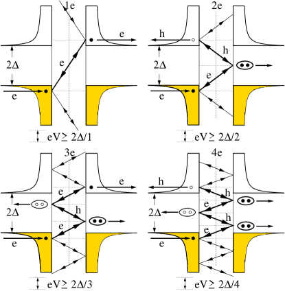
Figure 1: Schematic representation of the MARs for BCS superconductors with gap $\Delta$. We have sketched the density of states of both electrodes. In the upper left panel we describe the process in which a single electron tunnels through the system overcoming the gap due to a voltage $eV\geq 2\Delta$. The other panels show MARs of order $n=2,3,4$. In these processes an incoming electron at energy $E$ undergoes at least $n-1$ Andreev reflections to finally reach an empty state at energy $E+neV$. In these MARs a charge $ne$ is transferred with a probability, which for low transparencies goes as $T^{n}$. At zero temperature they have a threshold voltage $eV=2\Delta/n$. The arrows pointing to the left in the energy trajectories indicate that a quasiparticle can be normal reflected. The lines at energies below $E$ and above $E+neV$ indicate that after a detour a quasiparticle can be backscattered to finally contribute to the MAR of order $n$.

To arrive at these conclusions, we consider a voltage-biased superconducting point contact, i.e. two superconducting electrodes linked by a constriction, which is shorter than the coherence length and is described by a transmission probability $T$. To obtain the FCS in our system of interest we make use of the Keldysh-Green’s function approach to FCS introduced Nazarov and one of the authors Nazarov:99 ; Belzig2001 . The FCS of superconducting constrictions has the general form Belzig2001

$$S(\chi)=\frac{t_{0}}{h}{\textrm{Tr}}\ln\left[1+\frac{T}{4}\left(\{\check{G}_{1}(\chi),\check{G}_{2}\}_{\otimes}-2\right)\right]\;.$$ (2)

Here $\check{G}_{1(2)}$ denote matrix Green’s functions of the left and the right contact. The symbol $\otimes$ implies that the products of the Green’s functions are convolutions over the internal energy arguments, i.e. $(G_{1}\otimes G_{2})(E,E^{\prime})=\int dE_{1}\;G_{1}(E,E_{1})G_{2}(E_{1},E^{\prime})$. The trace runs not only over the Keldysh-Nambu space, but also includes integration energy. For a superconducting contact at finite bias voltage the CGF depends on time and Eq. (2) is integrated over a long measuring time $t_{0}$, much larger than the inverse of the Josepshon frequency.

Let us now describe the Green’s functions entering Eq. (2). The counting field $\chi$ is incorporated into the matrix Green’s function of the left electrode as follows

$$\check{G}_{1}(\chi,t,t^{\prime})=e^{-i\chi\check{\tau}_{K}/2}\check{G}_{1}(t,t^{\prime})e^{i\chi\check{\tau}_{K}/2}\,.$$ (3)

Here $\check{G}_{1}(t,t^{\prime})$ is the reservoir Green’s function in the absence of the counting field and $\check{\tau}_{\rm K}=\hat{\sigma}_{3}\bar{\tau}_{3}$ a matrix in Keldysh($\hat{\ }$)-Nambu($\bar{\ }$) space. We set the chemical potential of the right electrode to zero and represent the Green’s functions by $\check{G}_{1}(t,t^{\prime})=e^{ieVt\bar{\tau}_{3}}\check{G}_{S}(t-t^{\prime})e^{-ieVt^{\prime}\bar{\tau}_{3}}$ and $\check{G}_{2}(t,t^{\prime})=\check{G}_{S}(t-t^{\prime})$. Here, we have not included the dc part of the phase, since it can be shown that it drops from the expression of the dc FCS at finite bias. $\check{G}_{S}$ is the Green’s function of a superconducting reservoir (we consider the case of a symmetric junction), which reads

$$\check{G}_{S}(E)=\left(\begin{array}[c]{cc}(\bar{A}-\bar{R})f+\bar{R}&(\bar{A}-\bar{R})f\\ (\bar{A}-\bar{R})(1-f)&(\bar{R}-\bar{A})f+\bar{A}\end{array}\right).$$ (4)

Here $\bar{R}(\bar{A})(E)$ are retarded and advanced Green’s functions of the leads and $f(E)$ is the Fermi function. Advanced and retarded functions in (4) have the Nambu-structure $\bar{R}(\bar{A})=g^{\text{R,A}}\bar{\tau}_{3}+f^{\text{R,A}}\bar{\tau}_{1}$ fulfilling the normalization condition $f^{2}+g^{2}=1$. They depend on energy and the superconducting order parameter $\Delta$.

In Eq. (2) the matrix appearing inside the logarithm has an infinite dimension in energy space. In the case of N-N or N-S contacts such a matrix is diagonal in this space, which makes almost trivial the evaluation of the FCS. In the S-S case at finite bias this is no longer true, which introduces an enormous complication.

We now tackle the problem of how the functional convolution in Eq. (2) can be treated. The time-dependence of the Green’s functions leads to a representation of the form $\check{G}(E,E^{\prime})=\sum_{n}\check{G}_{0,n}(E)\delta(E-E^{\prime}+neV)$, where $n=0,\pm 2$. Restricting the fundamental energy interval to $E-E^{\prime}\in[0,eV]$ allows to represent the convolution as matrix product, i.e. $(G_{1}\otimes G_{2})(E,E^{\prime})\to(\check{G}_{1}\check{G}_{2})_{n,m}(E,E^{\prime})=\sum_{k}(G_{1})_{n,k}(E,E^{\prime})(G_{2})_{k,m}(E,E^{\prime})$. Writing the CGF as $S(\chi)=(t_{0}/h)\textrm{Tr}\ln\check{Q}$, where $\check{Q}=1+(\sqrt{T}/2)\left(\check{G}_{1}(\chi)-\check{G}_{2}\right)$ note . The trace in this new representation is written as $\int_{0}^{eV}dE\sum_{n}\textrm{Tr}\ln\left(\check{Q}\right)_{nn}$. In this way the functional convolution is reduced to matrix algebra for the infinite-dimensional matrix $\check{Q}$. Still, the task to compute ${\textrm{Tr}}\ln\check{Q}$ is nontrivial. However, noting that $\textrm{Tr}\ln\check{Q}=\ln\det\check{Q}$, it is obvious at this stage that $\det\check{Q}$ has the form of a Fourier series in $\chi$, which allows us to write the CGF as follows

$$S(\chi)=\frac{t_{0}}{h}\int^{eV}_{0}dE\;\ln\left[\sum^{n=\infty}_{n=-\infty}P^{\prime}_{n}(E,V)e^{in\chi}\right]\,.$$ (5)

Keeping in mind the normalization $S(0)=0$, it is clear that one can rewrite this expression in the form anticipated in Eq. (1), where the probabilities are given by $P_{n}(E,V)=P^{\prime}_{n}(E,V)/\sum^{n=\infty}_{n=-\infty}P^{\prime}_{n}(E,V)$. Of course, one has still to extract the expression of these probabilities from the determinant of $\check{Q}$, which is a non-trivial task. It turns out that $\check{Q}$ has a block-tridiagonal form, which allows to use a standard recursion technique. We define the following 4$\times$4 matrices

$$\check{F}_{\pm n} = \check{Q}_{\pm n,\pm n}-\check{Q}_{\pm n,\pm n\pm 2}\check{F}^{-1}_{\pm n\pm 2}\check{Q}_{\pm n\pm 2,\pm n}\;;\;n\geq 2$$

$$\check{F}_{0} = \check{Q}_{0,0}-\check{Q}_{0,-2}\check{F}^{-1}_{-2}\check{Q}_{-2,0}-\check{Q}_{0,2}\check{F}^{-1}_{2}\check{Q}_{2,0},$$ (6)

where $\check{Q}_{n,m}(E)=\check{Q}(E+neV,E+meV)$. With these definitions, $\det\check{Q}$ is simply given by $\det\check{Q}=\prod^{\infty}_{j=-\infty}\det\check{F}_{2j}$. In practice, $\det\check{F}_{n}=1$ if $|n|\gg\Delta/|eV|$. This reduces the problem to the calculation of the determinants of $4\times 4$ matrices.

In the zero-temperature limit one can work out this idea analytically to obtain the following expressions for the probabilities

$$P^{\prime}_{n}(E,V)=\sum^{n-1}_{l=0}K_{-n+l-2,l+2}\times J_{-n+l}(E)\times\left[\prod^{l-1}_{k=-n+l+1}(T/4)|f^{A}_{k}|^{2}\right]\times J_{l}(E)\;;\;\;n\geq 1$$

$$P^{\prime}_{0}(E,V)=K_{0,0}\times\left[Z_{0}^{R}\left(1+\frac{\sqrt{T}}{2}(g^{R}_{0}-g^{A}_{-1})-\frac{T}{4}(f^{A}_{-1})^{2}B^{A}_{-2}\right)-\frac{T}{4}(f^{R}_{0})^{2}\right]\times\Bigg{[}R\leftrightarrow A\Bigg{]}$$ (7)

Here, we have used the shorthand $g^{A,R}_{n}(E)\equiv g^{A,R}(E+neV)$, and defined

$$Z_{\pm n}^{\alpha}=1\pm\frac{\sqrt{T}}{2}(g^{\alpha}_{\pm(n+1)}-g^{\alpha}_{\pm n})-\frac{T}{4}(f^{\alpha}_{\pm(n+1)})^{2}B^{\alpha}_{\pm(n+2)}\;\;;\;\;n\geq 0\,,$$ (8)

where $\alpha=R,A$, $K_{n,m}=(\prod_{j=1}^{\infty}\det\check{F}_{n-2j})(\prod_{j=1}^{\infty}\det\check{F}_{m+2j})$ and the different functions can be expressed as follows

$$\left(B^{\alpha}_{\pm n}\right)^{-1} = 1\pm\frac{\sqrt{T}}{2}(g^{\alpha}_{\pm n}-g^{\alpha}_{\pm(n-1)})-\frac{T}{4}(f^{\alpha}_{\pm n})^{2}/Z^{\alpha}_{\pm n}\;;\;\det\check{F}_{\pm n}=\prod_{\alpha=A,R}\left[Z^{\alpha}_{\pm n}(1\pm\frac{\sqrt{T}}{2}(g^{\alpha}_{\pm n}-g^{\alpha}_{\pm(n-1)}))-\frac{T}{4}(f^{\alpha}_{\pm n})^{2}\right]$$

$$J_{\pm n} = \frac{\sqrt{T}}{2}(g^{A}_{\pm n}-g^{R}_{\pm n})\left[Z^{R}_{\pm n}Z^{A}_{\pm n}-\frac{T}{4}|f^{A}_{\pm n}|^{2}\right]\mp\frac{T}{4}(f^{A}_{\pm n}-f^{R}_{\pm n})\left[f^{R}_{\pm n}Z^{A}_{\pm n}+f^{A}_{\pm n}Z^{R}_{\pm n}\right]$$ (9)

Notice that, since at zero temperature the charge only flows in one direction, only the $P_{n}$ with $n\geq 0$ survive. It is worth stressing that the full information about the transport properties of superconducting point contacts is encoded in these probabilities. Let us remark that $P_{n}(E,V)$ are positive numbers bounded between 0 and 1. Although at a first glance they look complicated, they can be easily computed and provide the most efficient way to calculate the transport properties of these contacts. In practice, to determine the functions $B^{A,R}_{n}$ and $\det\check{F}_{n}$, one can use the boundary condition $B^{A,R}_{n}=\det\check{F}_{n}=1$ for $|n|\gg\Delta/|eV|$. For perfect transparency $(T=1)$ the previous expressions greatly simplify and the probabilities $P_{n}(E,V)$ can be written as

$$P_{n}=\sum^{n-1}_{l=0}(1-|a_{-n+l}|^{2})\left[\prod^{l-1}_{k=-n+l+1}|a_{k}|^{2}\right](1-|a_{l}|^{2}),$$ (10)

where $a(E)$ is the Andreev reflection coefficient defined as $a(E)=-if^{R}(E)/\left[1+g^{R}(E)\right]$, and $a_{n}=a(E+neV)$.

In view of Eqs. (Full Counting Statistics of Multiple Andreev Reflections-Full Counting Statistics of Multiple Andreev Reflections) the probabilities $P_{n}$ can be interpreted in the following way. $P_{n}$ is the probability of a MAR of order $n$, where a quasiparticle in an occupied state at energy $E$ is transmitted to an empty state at energy $E+neV$. The typical structure of the leading contribution to this probability consists of the product of three terms. First, $J_{0}$ gives the probability to inject the incoming quasiparticle at energy $E$. The term $\prod^{n-1}_{k=1}(T/4)|f^{A}_{k}|^{2}$ describes the cascade of $n-1$ Andreev reflections, in which an electron is reflected as a hole and vice versa, gaining an energy $eV$ in each reflection. Finally, $J_{n}$ gives the probability to inject a quasiparticle in an empty state at energy $E+neV$. In the tunnel regime $P_{n}(E,V)=(T^{n}/4^{n-1})\rho_{0}\rho_{n}\prod^{n-1}_{k=1}|f^{A}_{k}|^{2}$, $\rho(E)$ being the reservoir density of states. This interpretation is illustrated in Fig. 1, where we show the first four processes for BCS superconductors. The product of the determinants in the expression of $P^{\prime}_{n}$ (see Eq. (Full Counting Statistics of Multiple Andreev Reflections)) describes the possibility that a quasiparticle be reflected and make an excursion to energies below $E$ or above $E+neV$ Johansson1999 . In the tunnel regime this possibility is very unlikely and at perfect transparency is forbidden. As can be seen in Eq. (10), for $T=1$ the quasiparticle can only move upwards in energy due to the absence of normal reflection.

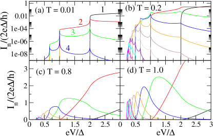
Figure 2: Current contribution of processes $n=1,...,10$, from right to left, as a function of voltage for BCS superconductors of gap $\Delta$. The different panels correspond to different transmissions. Notice the logarithmic scale in the upper panels.

From the knowledge of the FCS one can get a deep insight into the different transport properties by analyzing the role played by every process. For instance, in Fig. 2 we show the contribution to the dc current of the individual processes, i.e. $I_{n}=(2e/h)\int dE\;nP_{n}$, for the case of BCS superconductors of gap $\Delta$. In this case $f^{A,R}=i\Delta/\left[(E\mp i\delta)^{2}-\Delta^{2}\right]$, where $\delta=0^{+}$, and $g^{A,R}$ follows from normalization. As can be seen in Fig. 2, a MAR of order $n$ has a threshold voltage $eV=2\Delta/n$, below which it cannot occur. The opening of MARs at these threshold voltages is the origin of the pronounced subgap structure visible in the different transport properties (see Fig. 3). Notice also that at low transmission the MAR of order $n$ dominates the transport for voltages $[2\Delta/n,2\Delta/(n-1)]$, while at high transparencies several MARs give a significant contribution at a given voltage. This naturally explains why the effective charge is only quantized in the tunnel regime Cuevas1999 ; Cron2001 .

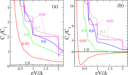
Figure 3: Second and third cumulant at zero temperature for a contact between BCS superconductors. Both are normalized to the first cumulant (the average current). The transmissions are indicated in the plots.

From the CGF one can easily calculate the cumulants of the distribution and in turn many transport properties. Of special interest are the first three cumulants $C_{1}=\overline{N}$, $C_{2}=\overline{(N-\overline{N})^{2}}$ and $C_{3}=\overline{(N-\overline{N})^{3}}$, which correspond to the average, width and skewness of the distribution, respectively. From the fact that the FCS is a multinomial distribution, it follows that at zero temperature these cumulants can be expressed in term of the probabilities $P_{n}(E,V)$ as $C_{n}(V)=\int^{eV}_{0}dE\;C_{n}(E,V)$, where

$$C_{1}(E,V)=\sum^{\infty}_{n=1}nP_{n}\;;\;C_{2}(E,V)=\sum^{\infty}_{n=1}n^{2}P_{n}-C^{2}_{1}(E,V)$$

$$C_{3}(E,V)=\sum^{\infty}_{n=1}n^{3}P_{n}-C_{1}(E,V)\left[C^{2}_{1}(E,V)+3C_{2}(E,V)\right].$$

The first two cumulants are simply related to the dc current, $I=(2e/h)C_{1}$, and to the zero-frequency noise $S_{I}=(4e^{2}/h)C_{2}$. In Fig. 3 we show $C_{2}$ normalized by $C_{1}$, which reproduces the results for the shot noise reported in the literature Cuevas1999 . In this figure we also show $C_{3}$. This cumulant determines the shape of the distribution, and it is attracting considerable attention Levitov2001 ; Reulet2003 because it contains information on nonequilibrium physics even at temperatures larger than the voltage. As seen in Fig. 3, at low transmissions $C_{3}=q^{2}C_{1}$, where $q(V)=1+\mbox{Int}(2\Delta/eV)$ is the charge transferred in the MAR which dominates the transport at a given voltage. This relation is a striking example of the general relation conjectured in Ref. Levitov2001 , and it is simply due to the fact that the multinomial distribution becomes Poissonian in this limit. For higher transmissions this cumulant is negative at high voltage as in the normal state, where $C_{3}=T(1-T)(1-2T)$, but it becomes positive at low bias. This sign change is due to the reduction of the MAR probabilities at low voltage. After the sign change there is a huge increase of the ratio $C_{3}/C_{1}$, which is a signature of the charge transfer in large quanta. Finally, at $T=1$ the cumulants ($C_{n}$ with $n>1$) do not completely vanish due to the fact that at a given voltage different MARs give a significant contribution, and therefore their probability is smaller than one (see Fig. 2(d)).

In summary, we have demonstrated that in superconducting contacts at finite voltage the charge transport is described by a multinomial distribution of multiple charge transfers. This proves that in the MAR processes the charge is indeed transmitted in large quanta. We have obtained analytically the MAR probabilities at zero temperature, from which all the transport properties are easily computed. Our result constitutes the culmination of the recent progress in the understanding of MARs, which are a key concept in mesoscopic superconductivity.

We acknowledge discussions with Yu.V. Nazarov. JCC was financially supported by the DFG within the CFN and WB by the Swiss NSF and the NCCR Nanoscience.

References

- (1) Ya.M. Blanter and M. Büttiker, Phys. Rep. 336, 1 (2000).
- (2) L.S. Levitov and G.B. Lesovik, Pis’ma Zh. Eksp. Teor. Fiz. 58, 225 (1993)]. L.S. Levitov, H.W. Lee, and G.B. Lesovik, J. Math. Phys. 37, 4845 (1996).
- (3) Quantum Noise in Mesoscopic Physics, edited by Yu.V. Nazarov (Kluwer, Dordrecht, 2003).
- (4) Yu.V. Nazarov, Ann. Phys. (Leipzig) 8, SI-193 (1999).
- (5) W. Belzig and Yu.V. Nazarov, Phys. Rev. Lett. 87, 197006 (2001); ibid 87, 067006 (2001).
- (6) T.M. Klapwijk, G.E. Blonder and M. Tinkham, Physica B 109&110, 1657 (1982).
- (7) E.N. Bratus et al., Phys. Rev. Lett. 74, 2110 (1995). D. Averin and A. Bardas, Phys. Rev. Lett. 75, 1831 (1995). J.C. Cuevas, A. Martín-Rodero and A. Levy Yeyati, Phys. Rev. B 54, 7366 (1996).
- (8) J.C. Cuevas, A. Martín-Rodero and A. Levy Yeyati, Phys. Rev. Lett. 82, 4086 (1999). Y. Naveh and D.V. Averin, Phys. Rev. Lett. 82, 4090 (1999).
- (9) E. Scheer et al., Phys. Rev. Lett. 78, 3535 (1997).
- (10) E. Scheer et al., Nature 394, 154 (1998).
- (11) R. Cron et al., Phys. Rev. Lett. 86, 4104 (2001).
- (12) We haved used to write the CGF as , where . Both terms give the same contribution and we concentrate in the analysis of the first one, and we drop the subindex .
- (13) G. Johansson et al., Superlatt. Microstruct. 25, 905 (1999).
- (14) L.S. Levitov and M. Reznikov, cond-mat/0111057.
- (15) B. Reulet, J. Senzier, D.E. Prober, cond-mat/0302084.