Five-loop $\epsilon$ expansion for $O(n)\times O(m)$ spin models

Abstract

We compute the Renormalization Group functions of a Landau-Ginzburg-Wilson Hamiltonian with O$(n)\times$O$(m)$ symmetry up to five-loop in Minimal Subtraction scheme. The line $n^{+}(m,d)$, which limits the region of second-order phase transition, is reconstructed in the framework of the $\epsilon=4-d$ expansion for generic values of $m$ up to $O(\epsilon^{5})$. For the physically interesting case of noncollinear but planar orderings $(m=2)$ we obtain $n^{+}(2,3)=6.1(6)$ by exploiting different resummation procedures. We substantiate this results re-analyzing six-loop fixed dimension series with pseudo-$\epsilon$ expansion, obtaining $n^{+}(2,3)=6.22(12)$. We also provide predictions for the critical exponents characterizing the second-order phase transition occurring for $n>n^{+}$.

I INTRODUCTION

In the last years much effort has been dedicated in the qualitative understanding and quantitative description of frustrated spin systems with noncollinear order. Despite the intensive theoretical and experimental investigation, strongly debated issues remain open. In three dimensions it is not clear if systems as stacked triangular antiferromagnets (STAs) and Helimagnets should undergo a continuous phase transitions (named chiral) belonging to an unusual universality class and hence characterized by new values of critical exponents, or if the transition is first order (see Refs. [1, 2, 3, 4] as review).

Field-theoretical studies of such systems are based on the O$(n)\times$O$(m)$ symmetric Landau-Ginzburg-Wilson (LGW) Hamiltonian [5, 1]

$${\cal H}=\int d^{d}x\left\{{1\over 2}\sum_{a}\left[(\partial_{\mu}\phi_{a})^{2}+r\phi_{a}^{2}\right]+{1\over 4!}u_{0}\left(\sum_{a}\phi_{a}^{2}\right)^{2}+{1\over 4!}v_{0}\sum_{a,b}\left[(\phi_{a}\cdot\phi_{b})^{2}-\phi_{a}^{2}\phi_{b}^{2}\right]\right\},$$ (1)

where $\phi_{a}$ ($1\leq a\leq m$) are $m$ sets of $n$-component vectors. Whether $m\leq n$ and $v_{0}>0$, Eq. (1) describes $m$-dimensional spin orderings in isotropic $n$-spin space with the O$(n)\rightarrow$O$(n-m)$ pattern of symmetry breaking. Negative values of $v_{0}$ correspond to simple ferromagnetic or antiferromagnetic ordering, and to magnets with sinusoidal spin structures [1]. The condition $0<v_{0}<m/(m-1)u_{0}$ is required to have noncollinearity and the boundedness of the free energy. For $m=2$ the Hamiltonian (1) describes magnets with noncollinear but planar orderings as frustrated $XY$ ($n=2$) and Heisenberg ($n=3$) antiferromagnets, while for $m\geq 3$ systems with noncoplanar ground states [6, 1].

The RG flow has always two fixed points (FP’s), the Gaussian one $(u_{0}=v_{0}=0)$ and the $O(nm)$ one $(v_{0}=0)$, while other two FP’s (called chiral and antichiral) appear for some values of $n$. At fixed $m$, for the physically relevant case $m\geq 1$, the $\epsilon$ expansion predicts four different regimes characterized as follows [7]:

• For $n>n^{+}(m,d)$, there are four FP’s, and the chiral one is stable.

• For $n^{-}(m,d)<n<n^{+}(m,d)$, only the Gaussian and the Heisenberg O($nm$)-symmetric FP’s are present, and none of them is stable. Thus the system is expected to undergo a first-order phase transition.

• For $n_{H}(m,d)<n<n^{-}(m,d)$, there are again four FP’s. However for $m<7$ the stable FP is in the region $v<0$ and the transition for those systems with $v_{0}>0$ is again first order.

• For $n<n_{H}(m,d)$, there are again four FP’s, and the Heisenberg O$(nm)$-symmetric one is stable.

For $m\geq 3$ all field theoretical (FT) methods ($\epsilon=4-d$ [6, 10], $1/n$ [10, 11], fixed dimensional $d=3$ [12], $\tilde{\epsilon}=d-2$[13] expansions, and the Effective Average Action Method (EAAM) [14]) agree indicating the existence of a marginal number of components of the order parameter $n^{+}(m,3)$ above which a second-order phase transition is driven by a stable chiral FP.

For $m=2$, again all the above mentioned FT methods indicate the existence of $n^{+}(2)\sim 6$ above which we expect a continuous phase transition [15, 10, 11, 13, 16, 17, 18, 19, 20, 25, 26, 27]. Instead, for $n<n^{+}$ the situation is controversial. Several magnetic materials that are supposed to be described by the Hamiltonian (1) with $n=2,3$ display scaling laws, but with experimental measured exponents that apparently depend on the material and sometimes also from the measure (see e.g. the recent experimental works [21] and also Refs. [3, 4] for an exhaustive list of experiments). The same scenario is found in MC simulations: systems like STA display scaling with almost well defined exponents [22] (see also [23] as the only simulation where apparently there is a first-order transition in STA), whereas systems with the same symmetry like rigid STA (STAR) and Stiefel $V_{n,2}$ (see e.g. Ref. [4] for the definition of these systems) clearly undergo first-order transition for $n=2,3$ [24]. Unfortunately a lot of theoretical efforts have not yet produced a unified picture. EAAM does not provide any stable FP favoring a weak first-order phase transition with nonuniversal pseudo-critical exponents [25, 26, 27, 4] that are in rough agreement with those coming from scaling relation found in experiments and Monte Carlo simulations. Whereas in six-loop fixed dimension approach another marginal number of components of the order parameter $N_{c2}<n^{+}$ exists [20], so that for $N_{c2}<n<n^{+}$ there is no stable FP, while for $n<N_{c2}$ a stable (focus-like) chiral FP appears [18, 19]. Since $N_{c2}=5.7(3)$ [20], according to this scenario, $XY$ and Heisenberg frustrated antiferromagnets undergo a second-order phase transition, if they are in the domain of attraction of the stable FP. The found critical exponents [18, 28] are in rough agreement with Monte Carlo and experimental results. Anyway, the continuous phase transition at this FP is very peculiar: scaling properties are governed over several decades of temperatures, by preasymptotic effective exponents, which can differ significantly from the asymptotic ones, explaining in this manner the apparently scattering experimental and numerical results [19]. Note that the existence of a stable FP does not exclude the possibility that some systems may undergo a first-order transition. Indeed, they may lie outside the attraction domain of the stable FP. According to mean-field arguments the systems undergoing second-order phase transition are those characterized by $v_{0}/u_{0}<m/(m-1)$. Since RG iterations may only narrow this region, systems that are outside this region surely undergo a first-order phase transition.

The stable FP found in fixed dimension for $n<N_{c2}$ is unrelated to the small-$\epsilon$ and large-$n$ chiral one. This fact does not imply an inconsistency of all perturbative results, since $\epsilon$ and $1/n$ expansions describe adiabatic moving from 4 dimensions and $n=\infty$ respectively and they are probably inadequate to describe the essentially three-dimensional features of the chiral FP for physical systems.

TABLE I.: Values of $n^{+}(m,3)$ for $m=2,3,4,5$ obtained with different FT methods.

	Method	m=2	m=3	m=4	m=5
Ref. [32]1994	Local Potential Approximation	$\sim 4.7$
Ref. [16]1994	$d=3$ expansion: $O(g^{4})$	3.91(1)
Ref. [15]1995	$\epsilon$ expansion: $O(\epsilon^{3})$	3.39
Ref. [25]2000	EAAM	$\sim 4$
Ref. [27]2001	EAAM	$\sim 5$
Ref. [10]2001	$1/n$ expansion: $O(1/n^{3})$	5.3	7.3	9.2	11.1
Ref. [10]2001	$\epsilon$ expansion: $O(\epsilon^{3})$	5.3(2)	9.1(9)	12(1)
Ref. [11]2002	$1/n$ expansion: $O(1/n^{2})$	$\sim 3.24$
Ref. [20]2003	$d=3$ expansion: $O(g^{7})$	6.4(4)	11.1(6)	14.7(8)	18(1)
This work	$\epsilon$ expansion: $O(\epsilon^{5})$	6.1(6)	9.5(5)	12.7(7)	15.7(1.0)
This work	pseudo-$\epsilon$ expansion: $O(\tau^{6})$	6.22(12)	9.9(3)	13.2(6)	16.3(1.3)

In recent years many efforts have been made to obtain a precise determination of $n^{+}(3,m)$. A complete list of results may be found in Table I. These scattered results clearly indicate that the extrapolation of low order $1/n$ and $\epsilon$ expansion predictions up to physical values of $n$ and $\epsilon$ is a quite delicate matter. For this reason we extend the knowledge of the RG function up to five-loop in $\epsilon$ expansion. Furthermore, to improve the goodness of fixed-dimensional $d=3$ estimates we re-analyze the six-loop perturbative series [18, 12] with the pseudo-$\epsilon$ expansion trick [29], since in many cases this method provided the most accurate results in the determination of the marginal number of order parameter components (see Ref. [30] for the cubic model and Ref. [31] for the weakly diluted $m$-vector model). We anticipate that also in this case the final estimate is very precise, as clear from Table I.

The paper is organized as follows. In Section II we determine $n^{\pm}(m,3)$ for several $n$ by means of five-loop $\epsilon$ expansion. Pseudo-$\epsilon$ expansion is considered in Section III. Section IV summarizes our results. In the Appendix A we report the estimates of the exponents for $m=2$ and $n\geq n^{+}(2,3)$, whereas in the Appendix B details of series computation are presented, and the Appendix C reports analytic forms of some quantities given in the text.

II Five-loop $\epsilon$-expansion

We extend the three-loop $\epsilon$ expansion of Refs. [15, 10] for the RG functions of the O($n$)$\times$O($m$) symmetric theory to five-loop. The obtained series and some details of calculations are reported in the Appendix B. Within these series, the $\epsilon$ expansion of $n^{\pm}(m,4-\epsilon)$ may be calculated to $O(\epsilon^{5})$. They are expanded as

$$n^{\pm}(m)=n_{0}^{\pm}(m)+n_{1}^{\pm}(m)\,\epsilon+n_{2}^{\pm}(m)\,\epsilon^{2}+n_{3}^{\pm}(m)\,\epsilon^{3}+n_{4}^{\pm}(m)\,\epsilon^{4}+O(\epsilon^{5}),$$ (2)

and the coefficients $n_{i}^{\pm}(m)$ may be obtained by requiring

$$\beta_{u}(u^{*},v^{*};n^{\pm})=0,\qquad\qquad\beta_{v}(u^{*},v^{*};n^{\pm})=0,$$ (3)

and

$${\rm det}\,\left|{\partial(\beta_{u},\beta_{v})\over\partial(u,v)}\right|(u^{*},v^{*};n^{\pm})=0.$$ (4)

Note that the previous equation is not the only possible choice to find $n^{\pm}$, one can e.g. impose the coincidence of the coordinates of the chiral and antichiral FP etc. However this was the most advantageous from the computational point of view. For generic values of $m$, the results obtained for the location of the FP’s and for $n^{\pm}(m)$ are too cumbersome in order to be reported here, thus we report them only at fixed $m=2,\,3$.

A Noncollinear but planar ordering: m=2

Let us first consider the physically relevant case $m=2$. The numerical expression for $n^{\pm}(2,4-\epsilon)$ simplifies to (their analytical expressions are in App. C)

$$n^{+}(2,4-\epsilon) = 21.7980-23.4310\,\epsilon+7.0882\,\epsilon^{2}-0.0321\,\epsilon^{3}+4.2650\,\epsilon^{4}+O(\epsilon^{5})\,,$$ (5)

$$n^{-}(2,4-\epsilon) = 2.2020-0.5690\,\epsilon+0.9892\,\epsilon^{2}-2.2786\,\epsilon^{3}+6.5406\,\epsilon^{4}+O(\epsilon^{5})\,.$$ (6)

The first three terms of the expansions are in agreement with previous works [15, 10]. In order to give a numerical estimate of $n^{\pm}(2,3)$ such series should be evaluated at $\epsilon=1$. A direct sum is obviously not effective since the series are clearly divergent. The series $n^{-}(2,4-\epsilon)$ has a quite regular behavior in $\epsilon$, with the last terms approximately factorial growing and with alternating sign coefficients. Thus a Padé-Borel-Leroy (PBL) resummation (see App. B) should be effective, and in fact it provides $n^{-}(2,3)=1.968(1)$. Despite to the stability of the result, this estimate cannot be right. Indeed we known, from the mapping onto the tetragonal model [16], that for $n=m=2$ a couple of FP’s exists in the $\epsilon$ expansion, thus $n^{-}(2,3)\geq 2$ holds. A direct analysis of three-dimensional six-loop series shows that $n^{-}(2,3)$ is a bit larger than 2 [33]. This was firstly noted in Ref. [16]. Anyway the precise value of $n^{-}(2,3)$ is not of interest for frustrated models and this disagreement will be not more commented below. We only quote it to show that PBL method apparently underestimates the final error bar.

TABLE II.: Non-defective PBL results for $n^{+}(m=2,3)$. The estimate from these data is $5.47(7)$.

Loop	3	4		5
Padé	[1/1]	[1/2]	[2/1]	[1/3]	[3/1]
b=0	3.385	4.477	5.423	5.402	5.455
b=1	3.514	4.593	5.423	5.586	5.455
b=2	3.583	4.654	5.423	5.688	5.455
b=3	3.626	4.693	5.423	5.753	5.455

The evaluation of $n^{+}(2,3)$ is much more difficult because of its irregular behavior. The results of PBL resummations are shown in Table II for several approximants. The fifth order ones indicate $n^{+}(2,3)=5.47(7)$ (it is the average and the variance of the approximants [1/3] and [3/1] with $b=0,1$). Anyway the previous analysis of $n^{-}(2,3)$ suggests that PBL method underestimates error bars, thus to have a more reliable result, we apply other summation methods to evaluate $n^{+}(2,3)$, that in practice allow one to extract better behaved series from Eq. (5). In what follows we present three different functions of $n^{+}(2,3)$ that behave better than Eq. (5). The choice of the functions is motivated or by physical reasons (as Eq. (9)) or by the experience in resumming divergent series (as Eq. (7)). Obviously we do not exclude the possibility of better choices.

The first function (as usually done for critical exponents) is

$${1\over n^{+}(2,4-\epsilon)}=0.0459+0.0493\epsilon+0.0381\epsilon^{2}+0.0250\epsilon^{3}+0.0056\epsilon^{4}+O(\epsilon^{5})\,,$$ (7)

whose coefficients decrease rapidly. Setting $\epsilon=1$, without resummation, one obtains $n^{+}(2,3)=7.50$ (at 3-loop), $n^{+}(2,3)=6.31$ (at 4-loop), and $n^{+}(2,3)=6.10$ (at 5-loop).

Another method, firstly employed in Ref. [10], use the knowledge of $n^{+}(2,2)$ to constrain the analysis at $\epsilon=2$, under the assumption that ${n^{+}}(m,d)$ is sufficiently smooth in $d$ at fixed $m$. In Ref. [10] it is assumed that the two-dimensional LGW stable FP is equivalent to that of the NL$\sigma$ model for all $n\geq 2$, $m\geq 2$, except $n=2$, $m=2$. Since the NL$\sigma$ model is asymptotically free, the authors of Ref. [10] conclude that $n^{+}(2,2)=2$. The knowledge of ${n}^{+}(2,2)$ may be exploited in order to obtain some informations on $n^{+}(2,3)$, rewriting $n^{+}(2,4-\epsilon)$ as

$$n^{+}(2,4-\epsilon) = 2+(2-\epsilon)(9.8990-6.7660\epsilon+0.1611\epsilon^{2}+0.0645\epsilon^{3}+2.1648\epsilon^{4})+O(\epsilon^{5})$$ (8)

$$= 2+(2-\epsilon)\,a(m=2,\epsilon).$$ (9)

Since the coefficients of $a(2,\epsilon)$ do not decrease, we consider $1/a(2,\epsilon)$ obtaining the more “convergent” expression

$${1\over a(2,\epsilon)}=0.1010+0.0690\epsilon+0.0456\epsilon^{2}+0.0294\epsilon^{3}-0.0032\epsilon^{4}+O(\epsilon^{5}),$$ (10)

which, setting $\epsilon=1$, gives $n^{+}(2,3)=6.64$ at three loop, $n^{+}(2,3)=6.08$ at four loop, and $n^{+}(2,3)=6.136$ at five loop.

Actually the exact value of $n^{+}(2,2)$ is a controversial matter, in fact it was pointed out that $Z_{2}$-type topological defects may lead to a finite-temperature phase transition in the two-dimensional $O(3)\times O(2)$ model (see e.g. Refs. [34, 35] and references therein, for different scenarios about the critical behavior of this model). Independently from the fact that the perturbative LGW approach is able to describe such topological excitations (that is still a very controversial point), one should expect as naive upper bound $n^{+}(2,2)=4$, since for $n\geq 4$ the NL$\sigma$ surely works. Using as constraint first $n^{+}(2,2)=2$ and then $n^{+}(2,2)=4$ one should kept in between the right value. Taking $n^{+}(2,2)=4$ and considering again the series of the inverse of the resulting $a(2,\epsilon)$, we have $n^{+}(2,3)=7.57$ at three loop, $n^{+}(2,3)=6.91$ at four loop, and $n^{+}(2,3)=6.70$ at five loop. The five-loop results with imposing $n^{+}(2,2)=2$ and $n^{+}(2,2)=4$ are quite close, signaling a weak dependence from the exact value of $n^{+}(2,2)$ and making the constrained analysis quite safe.

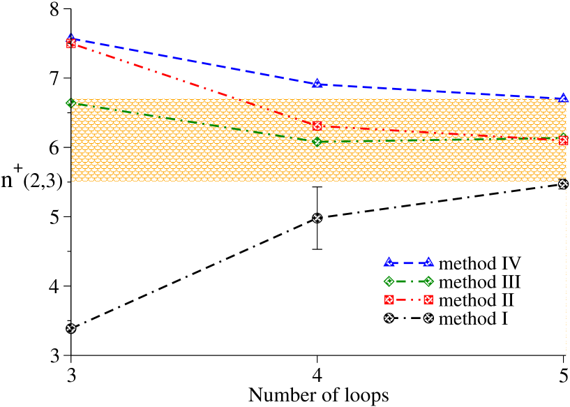
FIG. 1.: Different estimates of $n^{+}(2,3)$ with varying the number of loops. Method I is PBL, method II is Eq. 7, method III is Eq. 10, and method IV is the same of III, but with $n^{+}(2,2)=4$. The shadow region is our final estimate $n^{+}(2,3)=6.1(6)$.

In order to give a final estimate with a proper error bar, we report in Fig. 1 all our results. It appears that all the employed summation methods are slowly converging to the same asymptotic value, in particular PBL converges from below, while the other three from above and quickly. Note in particular that Eq. (10) (method II in figure) is quite flat up to the considered order, suggesting a good convergence. We take as final estimate the very conservative one $n^{+}(2,3)=6.1(6)$, which includes all five-loop data. The PBL result is only marginally compatible with the final estimate, but this is not surprising since PBL is the method that converges slowly and it is expected to underestimate error bars from the analysis of $n^{-}(2,3)$ (note also that the three-loop PBL 3.39 is the almost half of the common accepted value). The final value is only marginally compatible with the three-loop estimate $5.3(2)$ of Ref. [10]. Furthermore our quoted error is three times bigger than the three-loop one. We believe that our estimate is safe, contrarily to Ref. [10] were probably the valuation of the error bar was too optimistic.

The problem of the value of $n^{+}(2,2)$ may be also exploited resumming the series for $n^{+}$ at $\epsilon=2$, assuming a smooth dependence on $d$ up to $\epsilon=2$. The behavior of the series is worst than that for $\epsilon=1$, in fact Eqs. (7) and (9) are not effective anymore. However we can obtain useful informations from PBL method. The approximants [1/1], [1/2], and [1/3] give negative values and must be discarded. Only two working approximants remain, namely the [2/1] which leads to $n^{+}(2,2)=3.0$ and the [3/1] providing $n^{+}(2,2)=3.3$, independently from $b$. As a consequence we have a weak indication for $n^{+}(2,2)$ greater than the conjectured value $2$.

B Nonplanar ordering: m=3

Let us now consider the case $m=3$ which is relevant for spin systems which possess nonplanar orderings of the ground state. One possible example of such noncoplanar criticality was supposed to be the pyrochlore antiferromagnets FeF₃ [36] and [1] (page 4733). The coefficients $n_{i}^{\pm}(3)$ are (the analytic expressions are in the Appendix C)

$$n^{+}(3,4-\epsilon) = 32.4919-33.7184\epsilon+11.1002\epsilon^{2}-2.1440\epsilon^{3}+5.2756\epsilon^{4}+O(\epsilon^{5}),$$ (11)

$$n^{-}(3,4-\epsilon) = 1.5081-0.2816\epsilon+0.5827\epsilon^{2}-1.4192\epsilon^{3}+4.0193\epsilon^{4}+O(\epsilon^{5}).$$ (12)

Again for $\epsilon=1$, PBL technique for $n^{-}(3,3)$ seems very stable, leading to $n^{-}(3,3)=1.409(1)$. For $n^{+}(3,3)$ we can repeat the same analyses used for $m=2$. The PBL results are reported in Tab. III. In this case they are much more sensitive to the used approximant and a reliable estimate is difficult. Anyway this analysis suggests $n^{+}\sim 9$.

TABLE III.: Non-defective PBL results for $n^{+}(m=3,3)$.

Loop	3	4		5
Padé	[1/1]	[1/2]	[2/1]	[1/3]	[3/1]
b=0	6.448	7.591	8.152	8.621	9.176
b=1	6.654	7.705	8.134	8.834	9.191
b=2	6.763	7.760	8.123	8.954	9.202
b=3	6.831	7.792	8.116	9.031	9.209

As for $m=2$, the situation is better with considering

$${1\over n^{+}(3,4-\epsilon)}=0.0308+0.0319\,\epsilon+0.0226\,\epsilon^{2}+0.01460\,\epsilon^{3}+0.0045\,\epsilon^{4}+O(\epsilon^{5}),$$ (13)

which gives rise to $n^{+}(3,3)=11.7$ at three-loop, $n^{+}(3,3)=10.0$ at four-loop and $n^{+}(3,3)=9.57$ at five-loop.

Following Ref. [10] we impose in the constrained analysis only $n^{+}(3,2)=2$, since (at least for what we known) this value was never criticized in literature. We obtain

$$n^{+}(3,4-\epsilon) = 2+(2-\epsilon)\,(15.2460-9.2362\,\epsilon+0.9320\,\epsilon^{2}-0.6060\,\epsilon^{3}+2.3348\,\epsilon^{4})+O(\epsilon^{5})$$ (14)

$$= 2+(2-\epsilon)\,a(m=3,\epsilon)\,,$$ (15)

and again

$${1\over a(3,\epsilon)}=0.0656+0.0397\epsilon+0.0201\epsilon^{2}+0.0123\epsilon^{3}-0.0022\epsilon^{4}+O(\epsilon^{5}),$$ (16)

has a better behavior, giving at $\epsilon=1$, $n^{+}(3,3)=9.975$, $n^{+}(3,3)=9.26$, $n^{+}(3,3)=9.38$ at three-, four-, and five-loop respectively.

The data are much more scattered than those for $m=2$. A possible estimate, which includes the majority of the previously obtained results, is $n^{+}(3,3)\sim 9.5(5)$, that is lower than the six-loop fixed-dimension prediction $n^{+}(3,3)=11.1(6)$ [12].

In order to give a complete picture of the critical behavior for all values of $n$ and $m$, we calculate the expansion of $n^{+}(m,4-\epsilon)$ $m=4,5$, obtaining (applying the same summation methods of before) $n^{+}(4,3)=12.7(7)$ and $n^{+}(5,3)=15.7(1.0)$, that are the values reported in Table I. These results and their comparison with fixed dimension ones will be commented in the Conclusions.

III Pseudo $\epsilon$ expansion for ${n^{+}(m,3)}$

In this section we re-analyze the six-loop three-dimensional series of Refs. [18, 12] with the pseudo-$\epsilon$ expansion trick, since, as we have mentioned in the Introduction, it provided very good results for the marginal spin dimensionality in other models.

The idea behind this trick is very simple: one has only to multiply the linear terms of the two $\beta$ functions by a parameter $\tau$, find the FP’s (i.e. the common zeros of the $\beta$’s) as series in $\tau$ and analyze the results as in the $\epsilon$ expansion. If one is interested in the critical exponents, they are obtained as series in $\tau$ inserting the FP expansion in the appropriate RG functions. With this trick the cumulation of the errors coming from the non-exact knowledge of the FP and from the uncertainty in the resummation of the exponents is avoided, obtaining very precise results. Note that now, differently from $\epsilon$ expansion, only the value at $\tau=1$ makes sense. The only drawback of this trick is that it is unable to capture physical features of the systems that appear at higher perturbative orders. In fact at one-loop the series are equal (apart a normalization) to those of the $\epsilon$ expansion. Thus the FP’s structure may not be different from that of $\epsilon$ expansion. All the remarks and the limits of $\epsilon$-expansions apply also to pseudo-$\epsilon$ one. Explicitly the pseudo-$\epsilon$ expansion is able only to evaluate $n^{\pm}(m,3)$ and $n_{H}(m,3)$ but not $N_{c2}$. For this reason the pseudo-$\epsilon$ expansion is unable to recover the critical behavior for $m=2$ and $n=2,3$ coming from fixed dimensional field theory, even if it is a re-analysis of the same series.

For $m=2$ we obtain

$$n^{+}(2,3)=21.7980-15.6206\,\tau+0.2621\,\tau^{2}-0.1509\,\tau^{3}-0.0392\,\tau^{4}-0.0299\,\tau^{5}+O(\tau^{6})\,.$$ (17)

At least up to the presented number of loops the series does not behave as asymptotic ones with factorial growth of coefficients and alternating signs. So one may apply a simple Padé resummation of the series. The results are displayed in Tab. IV. Several approximants have poles on the positive real axis (these Padé are the underlined numbers) close to $\tau=1$ and thus the estimates of $n^{+}$ on their basis should be considered unreliable. Anyway some of these defective approximants have poles “far” from $\tau=1$, where the series must be evaluated. Thus one may expect the presence of a pole not to influence the approximant at $\tau=1$. Indeed all such Padé results are very close since lower order. We choose as final estimate the average of those six-loop order Padé without poles at $\tau<2$ (excluding those with $N=0$, giving unreliable results), and as error bar we take the maximum deviation from the average of four- and five-loop Padé. Within this procedure we have $n^{+}(2,3)=6.22(12)$. In order to corroborate this value we resum the series even with the PBL. In this case only the three-loop [1,1] and the four-loop [2,1] approximants are nondefective, giving $n^{+}(2,3)=6.43$ and $n^{+}(2,3)=6.35$ respectively, in agreement with the Padé estimate at the same perturbative order. Anyway a six-loop estimate is not possible within PBL.

TABLE IV.: Padé table for the series $n^{+}(2,3)$. The underlined values come out from Padé which possess poles on the positive real axis. The location of the poles nearest to $\tau=1$ is reported in brackets. The final estimate is $n^{+}(2,3)=6.22(12)$.

	$N=0$	$N=1$	$N=2$	$N=3$	$N=4$	$N=5$
$M=0$	21.798	6.177	6.439	6.289	6.249	6.219
$M=1$	12.698	6.435	6.344	6.236{3.85}	6.123{1.31}
$M=2$	9.827	6.290{10.38}	6.230{3.04}	6.182{1.74}
$M=3$	8.463	6.247{5.81}	6.154{1.45}
$M=4$	7.695	6.217{3.87}
$M=5$	7.221

To find $n^{+}(m,3)$ for systems with nonplanar spin orderings, we apply the same procedure exploited for $m=2$ obtaining the following perturbative expressions up to $O(\tau^{6})$

$$n^{+}(3,3) = 32.4919-22.4789\,\tau+0.4633\tau^{2}-0.2628\tau^{3}-0.1429\,\tau^{4}-0.1123\tau^{5},$$ (18)

Again, to extract quantitative information from them, we apply the procedure of before and check the results with PBL method. The final estimates are displayed in Tab. I together with those coming from five-loop $\epsilon$ expansion and other field theoretical methods, also for $m=4,5$.

IV conclusions

We compute the Renormalization Group functions of a Landau-Ginzburg-Wilson Hamiltonian with O$(n)\times$O$(m)$ symmetry up to five-loop in Minimal Subtraction scheme. Such higher order computation allowed us to reconstruct with good precision the line $n^{+}(m,d)$ in $\epsilon$ expansion up to $O(\epsilon^{5})$. We have also re-analyzed six-loop fixed dimension series with pseudo-$\epsilon$ expansion. All the results for $n^{+}(m,3)$ with $m=2,3,4,5$ are reported in Table I. The results coming from the $1/n$ expansion are not so near in magnitude to the $\epsilon$ and pseudo-$\epsilon$ ones. Anyway, in this case $n^{+}$ is determined by perturbative series which are known only to $O(1/n^{2})$, the correction to the leading term is not small, and since $n^{+}$ is not expected to be large in magnitude, one is extrapolating the results to value of $n$ which could be dangerous. Also the agreement with previous three-loop $\epsilon$-expansion is not good. Anyway, as already stated in the text, we believe that the error quoted in previous three loop works Refs. [15, 10] was underestimated. Differently the agreement is good between all the higher order perturbative methods, i.e. direct six-loop fixed dimension, $\epsilon$, and pseudo-$\epsilon$ expansion. Note that the pseudo-$\epsilon$ results are between the five-loop $\epsilon$ expansion and direct six-loop fixed dimension ones and are the more credible since they are the more stable with changing the perturbative order.

For the physically interesting case of noncollinear but planar orderings $(m=2)$, we obtain $n^{+}(2,3)=6.1(6)$ from five-loop $\epsilon$ expansion and $n^{+}(2,3)=6.22(12)$ from six-loop pseudo-$\epsilon$ expansion. Note that the last value seems to exclude $n=6$ from the second-order phase transition region, in contradiction with Monte Carlo results  [17] and EAAM [27] . Anyway two remarks on this point are necessary. First, being $n^{+}(2,3)-6=0.22(12)$ small, the concept of pseudo-scaling discussed in Ref. [26, 4] applies and the transition is expected to be extremely weak first order, i.e. all RG trajectories are attracted toward a small domain where the flow is very slow. In such domain the system spends the majority of its RG time (making the correlation length very large) and scaling is partially recovered. Second, the estimate of $N_{c2}=5.7(3)$ is marginally compatible with 6, leaving the possibility of a second-order phase transition at $n=6$ in the scenario of Refs. [18, 19, 20]. Anyhow we should expect measured critical exponents for $n=6$ close to those at $n^{+}(2,3)$. Monte Carlo [17] and EAAM [27] provide $\nu=0.700(11)$, $\gamma=1.383(36)$, and $\nu\simeq 0.707$, $\gamma\simeq 1.377$ respectively, that are quite close, but definitely different from the FT perturbative results for $n=n^{+}$ $\nu_{n=n^{+}}=0.635(4)$ (see Appendix A). We believe that this apparent disagreement deserves further investigations.

A Critical exponents

TABLE V.: Critical exponents for $n>n^{+}(2,3)$. Values obtained with other FT methods are reported for comparison. The EAAM and MC results for $n=6$ are also reported

. $\nu$ $n=6$ $n=n^{+}$ $n=7$ $n=8$ $n=16$ $n=32$ This work 0.635(4) 0.71(4) 0.75(4) 0.89(4) 0.94(2) 6L FD[20] 0.68(2) 0.71(1) 0.863(4) 0.936(1) O$(1/n^{2})$ [10] 0.697 0.743 0.885 0.946 EAAM 0.707 MC 0.700(11) $\gamma$ $n=6$ $n=n^{+}$ $n=7$ $n=8$ $n=16$ $n=32$ This work 1.25(2) 1.39(6) 1.45(6) 1.75(4) 1.87(4) 6L FD[20] 1.31(5) 1.40(2) 1.70(1) 1.860(5) $O(1/n^{2})$ [10] 1.36 1.45 1.75 1.88 EAAM 1.377 MC 1.383(36) [$\omega_{1}$, $\omega_{2}$] $n=6$ $n=n^{+}$ $n=7$ $n=8$ $n=16$ $n=32$ This work [0,0.86(3)] [0.84(3),0.33(10)] [0.84(3),0.45(8)] [0.86(1),0.77(2)] [0.91(2),0.90(1)] 6L FD[20] [0.83(2),0.23(5)] [0.83(2),0.36(4)] [0.876(4),0.714(9)] [0.933(2),0.868(2)] O$(1/n)$ [11] [0.768, 0.537] [0.797,0.594] [0.899,0.797] [0.949,0.899]

The critical exponents are computed by expanding in power of $\epsilon$ the exponent series at the FP. Such a computation gives the exponents only for

$$n>n^{+}_{0}(m)=5m+2+2\sqrt{6(m+2)(m-1)},$$ (A1)

or

$$n<n^{-}_{0}(m)=5m+2-2\sqrt{6(m+2)(m-1)}.$$ (A2)

Indeed, if these bounds are not satisfied the FP’s are complex and therefore also the exponent series. This is actually only an artifact of the $\epsilon$ expansion and the exponents are real and well defined for $n>n^{+}(m,d)$ (see for details Refs. [7, 10]). In order to obtain series for the exponents in all the relevant domain we can perform the following trick [10]. For $n^{+}<n<n_{0}^{+}$ we set $n=n^{+}(m,4-\epsilon)+\Delta n$ and re-expand all series in powers of $\epsilon$ keeping $\Delta n$ fixed. In particular, for $\Delta n=0$ we obtain the critical exponents for $n=n^{+}$. In the most interesting case of $m=2$ the exponents along the line $n=n^{+}$ are (their analytic forms are in the App. C)

$$\eta_{n=n^{+}}=0.0208\,\epsilon^{2}+0.0174\,\epsilon^{3}+0.0061\,\epsilon^{4}+0.0032\,\epsilon^{5}+O(\epsilon^{6})\,,$$ (A3)

and

$$(\nu_{n=n^{+}})^{-1}=2-0.5\,\epsilon+0.0290\,\epsilon^{2}+0.0767\,\epsilon^{3}-0.0478\,\epsilon^{4}+0.0762\,\epsilon^{5}+O(\epsilon^{6})\,.$$ (A4)

After a PBL resummation we have $\nu_{n=n^{+}}=0.635(4)$ and $\eta_{n=n^{+}}=0.049(1)$. In the same way we have also estimated the subleading exponents governing the corrections to the scaling (i.e. the eigenvalues of the matrix (B4)). The smallest one is obviously $\omega_{1}^{n=n^{+}}=0$, instead the biggest one is $\omega_{2}^{n=n^{+}}=0.86(3)$, after PBL resummation. Now we may calculate critical exponents for all $n>n^{+}(2,3)$, even if $n<n_{0}^{+}(2)\simeq 21.8$. The resulting critical exponents have a double source of error: one coming from uncertainty in the resummation and one from the not precise knowledge of $n^{+}(2,3)$. Note that the latter dominates the given error for $n=7,8,16$, since the resummation of the exponents is very precise, contrarily to that of $n^{+}(2,3)$. To give an example, at $n=7$ we have $\Delta n=0.9(6)$, that leads to $\nu(\Delta n=0.3)\simeq 0.67$ and $\nu(\Delta n=1.5)\simeq 0.75$, and thus the resulting estimate $\nu(n=7)=0.71(4)$. All other exponents are calculated in the same way. For $n>n_{0}^{+}(2)$ a direct resummation of the critical exponents is possible. In Table V we report the results for $n=7,\,8,\,16,\,32$ and the corresponding six-loop fixed-dimension and $1/n$ ones for comparison. There is a quite good agreement between all FT methods, a part from the estimates of $\omega$ at $n=16,32$, that seems to differ significantly from fixed dimension results. The source of such disagreement is not completely clear to us. It may be due to an underestimating of the error (especially in fixed dimension), or to the bad behavior of the resummation. Anyway it is not so surprising, since already for the $O(n)$ model the estimates of $\omega$ are not very good (see e.g. Ref. [3]).

B Perturbative Series

We calculate the perturbative RG function in the minimal subtraction ($\overline{\rm MS}$) renormalization scheme for the massless theory. We compute the divergent part of the irreducible two-point functions of the field $\phi$, of the two-point correlation functions with insertions of the quadratic operators $\phi^{2}$, and of the two independent four-point correlation functions. The diagrams contributing to this calculation are 162 for the four-point functions and 26 for the two-point one. We handle them with a symbolic manipulation program, which generate the diagrams and compute the symmetry and group factors of each of them. We use the results of Ref. [37], where the primitive divergent parts of all integrals appearing in our computation are reported. We determine the renormalization constant $Z_{\phi}$ associated with the fields $\phi$, the renormalization constant $Z_{t}$ of the quadratic operator $\phi^{2}$, and the renormalized quartic couplings $u,v$. The functions $\beta_{u}$, $\beta_{v}$, $\eta_{\phi}$ and $\eta_{t}$ are determined using the relations

$$\beta_{u}(u,v)=\mu\left.{\partial u\over\partial\mu}\right|_{u_{0},v_{0}},\qquad\qquad\beta_{v}(u,v)=\mu\left.{\partial v\over\partial\mu}\right|_{u_{0},v_{0}},$$ (B1)

$$\eta_{\phi}(u,v)=\left.{\partial\log Z_{\phi}\over\partial\log\mu}\right|_{u_{0},v_{0}},\qquad\eta_{t}(u,v)=\left.{\partial\log Z_{t}\over\partial\log\mu}\right|_{u_{0},v_{0}}.$$ (B2)

The zeroes $(u^{*},v^{*})$ of the $\beta$ functions provide the FP’s of the theory. In the framework of the $\epsilon$ expansion, they are obtained as perturbative expansions in $\epsilon$ and then are inserted in the RG functions to determine the $\epsilon$ expansion of the critical exponents:

$$\eta=\eta_{\phi}(u^{*},v^{*}),\quad\nu=(2-\eta_{\phi}(u^{*},v^{*})+\eta_{t}(u^{*},v^{*}))^{-1}.$$ (B3)

The stability of each FP is controlled by the $2\times 2$ matrix

$$\Omega=\left(\matrix{\displaystyle\frac{\partial\beta_{u}(u,v)}{\partial\,u}&\displaystyle\frac{\partial\beta_{u}(u,v)}{\partial\,v}\cr\cr\displaystyle\frac{\partial\beta_{v}(u,v)}{\partial\,u}&\displaystyle\frac{\partial\beta_{v}(u,v)}{\partial\,v}}\right)\;.$$ (B4)

A stable FP must have two eigenvalues with positive real parts, while a FP possessing eigenvalues with nonvanishing imaginary parts is called focus.

In reporting the series we make explicit use of the symmetry under the exchange $(m,n)$ and write the RG functions as

$$\beta_{u}=\beta_{1}^{u}+\beta_{2}^{u}+\beta_{3}^{u}+\beta_{4}^{u}+\beta_{5}^{u}+\beta_{6}^{u}, \beta_{k}^{u}=\sum_{i=0}^{k}u^{i}v^{k-i}(U_{k-i,i}(m,n)+U_{k-i,i}(n,m)),$$ (B5)

$$\beta_{v}=\beta_{1}^{v}+\beta_{2}^{v}+\beta_{3}^{v}+\beta_{4}^{v}+\beta_{5}^{v}+\beta_{6}^{v}, \beta_{k}^{v}=\sum_{i=0}^{k}u^{i}v^{k-i}(V_{k-i,i}(m,n)+V_{k-i,i}(n,m)),$$ (B6)

$$\eta_{\phi}=\eta_{1}+\eta_{2}+\eta_{3}+\eta_{4}+\eta_{5}, \eta_{k}=\sum_{i=0}^{k}u^{i}v^{k-i}(E_{k-i,i}(m,n)+E_{k-i,i}(n,m)),$$ (B7)

$${1\over\nu}=\nu_{1}+\nu_{2}+\nu_{3}+\nu_{4}+\nu_{5}, \nu_{k}=\sum_{i=0}^{k}u^{i}v^{k-i}(B_{k-i,i}(m,n)+B_{k-i,i}(n,m)),$$ (B8)

where the first three orders coincide with those of Refs. [7, 6, 15, 10], and the four and five-loop coefficients are reported in Tabs. VI, VII, VIII, IX, X.

In order to verify the exactness of our perturbative series we perform several checks on them. They reduce to the existing $O(\epsilon^{5})$ ones for the O($N$)-symmetric theory [38] in the proper limit. For the particular case $n=m=2$ they agree, according to the exact mapping of Ref. [16], with the four-loop $\epsilon$ expansion of the so called tetragonal model Ref. [39]. The value of $n_{H}(m,4-\epsilon)$ coincides with $N_{c}/m$, where $N_{c}$ is the marginal spin dimensionality of the cubic model obtained in [40], according to the symmetry argument of Refs. [8, 9]. Finally, the $1/n$ expansion of the series coincides with the expansion close to four dimensions of the $1/n$ exponents of Refs. [10, 11].

Since the $\epsilon$ expansion is asymptotic, the series must be properly resummed to provide results for three-dimensional systems. The first method that is applied to those series that do not yet behave as asymptotic is Padé summation, which consists in extending the series analytically by the ratio of two polynomials. The approximant $[N/M](\tau)=\sum_{i=0}^{N}a_{i}\tau^{i}/\sum_{j=0}^{M}b_{j}\tau^{j}$ is determined by imposing the equivalence between its Taylor coefficients with the ones of the original series. We also use Padé-Borel-Leroy (PBL) resummation that works as follows. Let $S(\epsilon)=\sum\,s_{k}\epsilon^{k}$ be the quantity we want to resum. The Borel-Leroy transform of $S(\epsilon)$, is defined by $B_{b}(t)=\sum_{k}s_{k}t^{k}/\Gamma(k+b+1)$. In order to evaluate $S(\epsilon=1)$ it is necessary to perform an analytic continuation of $B_{b}(t)$, that may be achieved using Padé approximants $[N/M]$. Named $P_{S}(b,N,M)(t)$ such analytic continuation, estimates of $S(\epsilon)$ are given by

$$\int_{0}^{\infty}dt\,t^{b}e^{-t}P_{S}(b,N,M)(\epsilon\,t)\,,$$ (B9)

depending on the considered Padé $[N/M]$ and on the value of the free parameter $b$. Since the integral (B9) should be defined, the approximant must not have poles on the real positive axis. The Padé with real positive poles are called defective and must be discarded in the average procedure.

C Analytic expression

In this appendix we report some useful analytic expressions of the quantities reported in the text. We believe that analytical results are very useful for those who want to check our results or to compare with other methods where analytic limits are known.

The analytic expressions of Eqs. (5) are

$$n_{0}^{\pm}(2) = 12\pm 4\,{\sqrt{6}},$$ (C1)

$$n_{1}^{\pm}(2) = -12\mp{14\over 3}\,{\sqrt{6}},$$ (C2)

$$n_{2}^{\pm}(2) = \frac{274\pm 91\,{\sqrt{6}}}{300}+\frac{(156\pm 47\,{\sqrt{6}})}{60}\,\zeta(3)$$ (C3)

$$n_{3}^{\pm}(2) = \frac{72771\pm 23369\,{\sqrt{6}}}{67500}+\frac{(156\pm 47\,{\sqrt{6}})}{7200}\,{\pi}^{4}+\frac{(15004\pm 10621\,{\sqrt{6}})}{18000}\,\zeta(3)$$ (C5)

$$-\frac{(464\pm 107\,{\sqrt{6}})}{90}\,\zeta(5),$$

$$n_{4}^{\pm}(2) = \frac{61636782\pm 14010773\,{\sqrt{6}}}{162000000}+\frac{(15004\pm 10621\,{\sqrt{6}})}{2160000}\,{\pi}^{4}-\frac{(464\pm 107\,{\sqrt{6}})}{68040}\,{\pi}^{6}$$ (C8)

$$-\frac{86358388\pm 29909737\,{\sqrt{6}}}{21600000}\,\zeta(3)-\frac{7\,\left(84368\pm 38339\,{\sqrt{6}}\right)}{720000}\,\zeta(3)^{2}$$

$$+\frac{(2753732\pm 735873\,{\sqrt{6}})}{432000}\,\zeta(5)+\frac{49\,(1332\pm 119\,{\sqrt{6}})}{6400}\,\zeta(7),$$

and for Eqs. (11)

$$n_{0}^{\pm}(3) = 17\pm 4\,{\sqrt{15}},$$ (C9)

$$n_{1}^{\pm}(3) = -17\mp\frac{259\,{\sqrt{15}}}{60},$$ (C10)

$$n_{2}^{\pm}(3) = \frac{2267955\pm 461534\,{\sqrt{15}}}{2323200}+\frac{42741\pm 10183\,{\sqrt{15}}}{10560}\,\zeta(3),$$ (C11)

$$n_{3}^{\pm}(3) = \frac{141926963025\pm 31936343543\,{\sqrt{15}}}{101198592000}+\frac{42741\pm 10183\,{\sqrt{15}}}{1267200}\,\pi^{4}$$ (C13)

$$+\frac{184976182\pm 103127153\,{\sqrt{15}}}{306662400}\,\zeta(3)-\frac{4835795\pm 1072837\,{\sqrt{15}}}{696960}\,\zeta(5),$$

$$n_{4}^{\pm}(3) = \frac{17531276380245840\pm 3847065393512279\,{\sqrt{15}}}{47020913786880000}-\frac{4835795\pm 1072837\,{\sqrt{15}}}{526901760}\,\pi^{6}$$ (C17)

$$+\frac{184976182\pm 103127153\,{\sqrt{15}}}{36799488000}\,\pi^{4}-\frac{41214520769938\pm 9458643900547\,{\sqrt{15}}}{7124380876800}\,\zeta(3)$$

$$+\frac{1871364718325\pm 375167813937\,{\sqrt{15}}}{161917747200}\,\zeta(5)+\frac{49(210903545\pm 35255789\,{\sqrt{15}})}{1090355200}\,\zeta(7)$$

$$+\frac{739213610260\pm 238830577907\,{\sqrt{15}}}{539725824000}\,\zeta(3)^{2}\,.$$

Similarly for (A3), i.e. the exponents for $m=2$ and $n=n^{+}(2,4-\epsilon)$,

$$\eta_{n=n^{+}} = \frac{1}{48}\,\epsilon^{2}+\frac{5}{288}\,\epsilon^{3}+\left(\frac{-119+24\,{\sqrt{6}}}{14400}\zeta(3)+\frac{3691+124\,{\sqrt{6}}}{360000}\right)\,\epsilon^{4}$$ (C20)

$$+\left(\frac{6408547+408608\,{\sqrt{6}}}{1296000000}+\frac{-119+24\,{\sqrt{6}}}{1728000}\,\pi^{4}\right.$$

$$\left.+\frac{-324561+51976\,{\sqrt{6}}}{32400000}\zeta(3)+\frac{5739-1508\,{\sqrt{6}}}{259200}\zeta(5)\right)\epsilon^{5}+O(\epsilon^{6})\,,$$

and for (A4)

$${1\over\nu_{n=n^{+}}} = 2-{\epsilon\over 2}+\frac{-1+{\sqrt{6}}}{50}\epsilon^{2}+\left(\frac{37+4\,{\sqrt{6}}}{1000}\zeta(3)+\frac{397-37\,{\sqrt{6}}}{15000}\right)\epsilon^{3}+\left(\frac{1104341-315351\,{\sqrt{6}}}{18000000}\right.$$ (C25)

$$\left.+\frac{37+4\,{\sqrt{6}}}{120000}\pi^{4}+\frac{-112429+46574\,{\sqrt{6}}}{1800000}\zeta(3)-\frac{2473+484\,{\sqrt{6}}}{36000}\zeta(5)\right)\epsilon^{4}$$

$$+\left(\frac{19528133-6267483\,{\sqrt{6}}}{270000000}+\frac{-112429+46574\,{\sqrt{6}}}{216000000}\pi^{4}-\frac{2473+484\,{\sqrt{6}}}{27216000}\pi^{6}\right.$$

$$\left.-\frac{31404323-14177332\,{\sqrt{6}}}{216000000}\zeta(3)+\frac{76622-74335\,{\sqrt{6}}}{4500000}\zeta(3)^{2}\right.$$

$$\left.+\frac{4966979-1949164\,{\sqrt{6}}}{21600000}\zeta(5)+\frac{49\,\left(135+74\,{\sqrt{6}}\right)}{80000}\zeta(7)\right)\epsilon^{5}+O(\epsilon^{6})\,.$$

REFERENCES

- [1] H. Kawamura, J. Phys.: Condens. Matter 10 (1998) 4707 .
- [2] M. F. Collins and O. A. Petrenko, Can. J. Phys. 75 (1997) 605.
- [3] A. Pelissetto and E. Vicari, Phys. Rep. 368 (2002) 549.
- [4] B. Delamotte, D. Mouhanna, and M. Tissier, cond-mat/0309101.
- [5] D. R. T. Jones et al., J. Phys. C: Solid St. Phys. 9 (1976) 743; D. Bailin et al., J. Phys. C: Solid St. Phys. 10 (1977) 1159.
- [6] H. Kawamura, J. Phys. Soc. Japan 59 (1990) 2305.
- [7] H. Kawamura, Phys. Rev. B 38 (1988) 4916; erratum B 42 (1990) 2610.
- [8] P. Calabrese, A. Pelissetto, and E. Vicari, Phys. Rev. B 67 (2003) 054505.
- [9] P. Calabrese, A. Pelissetto, and E. Vicari, cond-mat/0306273; P. Calabrese, A. Pelissetto, P. Rossi, and E. Vicari, hep-th/0212161.
- [10] A. Pelissetto, P. Rossi and E. Vicari, Nucl. Phys. B 607 (2001) 605.
- [11] J. A. Gracey, Nucl. Phys. B 644 (2002) 433.
- [12] P. Parruccini, Phys. Rev. B 68 (2003) 104415.
- [13] P. Azaria, B. Delamotte and T. Jolicoeur, Phys. Rev. Lett. 64 (1990) 3175; P. Azaria, B. Delamotte, F. Delduc and T. Jolicoeur, Nucl. Phys. B 408 (1993) 485.
- [14] M. Tissier, D. Mouhanna, and B. Delamotte, Phys. Rev. B 61 (2000) 15327.
- [15] S. A. Antonenko, A. I. Sokolov, and K. B. Varnashev, Phys. Lett. A 208 (1995) 161.
- [16] S. A. Antonenko and A. I. Sokolov, Phys. Rev. B 49 15901 (1994).
- [17] D. Loison, A. I. Sokolov, B. Delamotte, S. A. Antonenko, K. D. Schotte, and H. T. Diep, Pis’ma Zh. Eksp. Teor. Fiz. 72 (2000) 487 [JETP Letters 72 (2000) 337].
- [18] A. Pelissetto, P. Rossi and E. Vicari, Phys. Rev. B 63 (2001) 140414.
- [19] P. Calabrese, P. Parruccini, and A. I. Sokolov, Phys. Rev. B 66 (2002) 180403.
- [20] P. Calabrese, P. Parruccini, and A. I. Sokolov, Phys. Rev. B 68 (2003) 094415.
- [21] A. Lascialfari et al., Phys. Rev. B 67 (2003) 224408; M. Fiebig, et al., Phys. Rev. Lett. 88 (2002) 027203; V. P. Plakhty et al., Phys. Rev. B 64 (2001) 100402(R); V. P. Plakhty et al., Phys. Rev. Lett. 85 (2000) 3942; G. C. DeFotis et al., Phys. Rev. B 65 (2002) 94403; R. Bügel et al., Phys. Rev. B 64 (2001) 94406; T. Ono et al., J. Phys. Cond. Matt. 11 (1999) 4427; T. Ono et al., J. Magn. Magn. Mat. 177-181 (1998) 735.
- [22] A. Peles and B. W. Southern, Phys. Rev. B 67 (2003) 184407; E. H. Boubcheur, D. Loison, and H.T. Diep, Rev. B 54 (1996) 4165; A. Mailhot, M. L. Plumer, and A. Caillé, Rev. B 50 (1994) 6854; D. Loison and H.T. Diep, Rev. B 50 (1994) 16453.
- [23] M. Itakura, J. Phys. Soc. Jap. 72 (2003) 74.
- [24] D. Loison and K. D. Schotte, Eur. Phys. J. B 5 (1998) 735; Eur. Phys. J. B 14 (2000) 125.
- [25] M. Tissier, B. Delamotte, and D. Mouhanna, Phys. Rev. Lett. 84 (2000) 5208.
- [26] M. Tissier, B. Delamotte and D. Mouhanna, Phys. Rev. B 67 (2003) 134422.
- [27] M. Tissier, B. Delamotte and D. Mouhanna, Int. J. Mod. Phys. A 16 (2001) 2131.
- [28] A. Pelissetto, P. Rossi and E. Vicari, Phys. Rev. B 65 (2002) 020403.
- [29] The pseudo- expansion was introduced by B. G. Nickel, see citation 19 in J. C. Le Guillou and J. Zinn-Justin, Phys. Rev. B 21 (1980) 3976.
- [30] R. Folk, Yu. Holovatch, and T. Yavors’kii, Phys. Rev. B 62 (2000) 12195.
- [31] Yu. Holovatch, M. Dudka, and T. Yavors’kii, J. Phys. Studies 5 (2001) 233.
- [32] G. Zumbach, Nucl. Phys. B 413 (1994) 771.
- [33] Unpublished.
- [34] P. Calabrese and P. Parruccini, Phys. Rev. B 64 (2001) 184408; P. Calabrese, E. V. Orlov, P. Parruccini, and A. I. Sokolov, Phys. Rev. B 67 (2003) 024413.
- [35] M. Caffarel et al., Phys Rev. B 64 (2001) 014412.
- [36] J. N. Reimers, J. Greedan, and M. Björgvinsson, Phys. Rev. B 45 (1992) 7295; A. Mailhot and M. L. Plumer Phys. Rev. B 48 (1993) 9881.
- [37] H. Kleinert and V. Schulte-Frohlinde, Critical Properties of -Theories (World Scientific, Singapore, 2001).
- [38] K. G. Chetyrkin, S. G. Gorishny, S. A. Larin, and F. V. Tkachov, Phys. Lett. B 132 (1983) 351; H. Kleinert, J. Neu, V. Schulte-Frohlinde, K. G. Chetyrkin, and S. A. Larin, Phys. Lett. B 272 (1991) 39; (E) B 319 (1993) 545.
- [39] A. I. Mudrov and K. B. Varnashev, Phys. Rev. B 64, (2001) 214423; JETP Letters 74, (2001) 279; J. Phys. A 34, (2001) L347.
- [40] H. Kleinert and V. Schulte-Frohlinde, Phys. Lett. B 342, 284 (1995).