Edge modes, edge currents, and gauge invariance in $p_{x}+ip_{y}$ superfluids and superconductors.

Abstract

The excitation spectrum of a two-dimensional $p_{x}+ip_{y}$ fermionic superfluid, such as a thin film of ³He-A, includes a gapless Majorana-Weyl fermion which is confined to the boundary by Andreev reflection. There is also a persistent ground-state boundary current which provides a droplet containing $N$ particles with angular momentum $\hbar N/2$. Both of these boundary effects are associated with bulk Chern-Simons effective actions. We show that the gapless edge-mode is required for the gauge invariance of the total effective action, but the same is not true of the boundary current.

I Introduction

Read and Green [1] have pointed out close parallels between two-dimensional $p_{x}+ip_{y}$ chiral fermionic superfluids (a thin film of ³He-A for example) and the $\nu=1/2$ Pfaffian quantum Hall state. The many-body ground-state wavefunction of both systems contains a Pfaffian factor, and both support gapless Majorana-Weyl edge modes [2]. In addition, both systems can host vortex defects with non-Abelian statistics [3, 4]. The $p_{x}+ip_{y}$ superfluid also possesses an equilibrium edge current that is consistent with an $\hbar$-per-Cooper-pair intrinsic angular momentum [5, 6, 7]. This current is similar to that induced by a confining potential at the boundary of a Hall droplet, and occurs because chiral fermionic superfluids manifest an analogue of the quantum Hall effect, even in the absence of an external magnetic field [8].

The principal differences between the Pfaffian Hall state and the chiral superfluid are that, in addition to the Pfaffian, the Hall-state wavefunction includes a symmetric $\nu=1/2$ Laughlin factor; also the Hall system is spin polarized, while the superfluid retains two active spin components. A less significant difference is that the Hall fluid is incompressible while a neutral superfluid like ³He-A has a gapless acoustic mode. This acoustic mode will, however, be gapped in a charged superfluid state, such as that believed to exist in the layered Sr₂RuO₄ superconductors [9, 10].

In the quantum Hall effect, the lack of low energy bulk degrees of freedom leads to the dynamics of the boundary and the bulk being intimately connected. Currents flowing in the the bulk serve to soak up the anomalies of the edge-mode conservation laws [11], and, more profoundly, the bulk many-body wavefunction can be constructed from the conformal blocks of the edge conformal field theory [3]. The existence of the conformally invariant Majorana edge mode suggests that something similar is true for the superfluid.

Because of the interest of quantum systems with non-Abelian statistics, both for their intrinsic appeal as exotic physics and for their potential application to quantum computing [12, 13], there is reason to search for the simplest possible description of their dynamics. Thus we seek an effective action which captures all the essential low-energy degrees of freedom of the system. The construction of such an effective action for the fermionic Pfaffian Hall state is, however, rather complicated [14]. It is therefore worth examining other systems with similar properties.

One such system is the bosonic Pfaffian quantum Hall state, which can perhaps be realized in rotating Bose condensates. The bosonic Pfaffian state has a ground-state wavefunction consisting of the product of the antisymmetric Pfaffian and an antisymmetric $\nu=1$ Laughlin factor, making it even under particle interchange. In this case [14, 15] the effective action is an $SU(2)$ Chern-Simons term at level $k=2$. This means that the edge states form representations of an ${SU(2)}_{2}$ current algebra. Indeed, the space of low energy states is spanned by wavefunctions consisting of polynomials in the complex coordinates $z_{i}$ that vanish when any three of the $z_{i}$ coincide. The generating function for the number of such polynomials is a character of the ${SU(2)}_{2}$ algebra [16].

The $p_{x}+ip_{y}$ superfluid is also relatively easy to analyze because its effective action has been computed by standard gradient expansion methods [8, 17]. It is the purpose of this paper to explore some of the mathematical and physical aspects of the resulting expression. We will see that the response of the fluid to a non-Abelian gauge field which couples to the spin degree of freedom is governed by a Chern-Simons term of conventional form, but with a coefficient corresponding to level $k={\textstyle{1\over 2}}$. Since invariance under “large” gauge transformations demands that the level $k$ be an integer, this means that the spin action cannot be gauge invariant on its own. Gauge invariance is restored only when we take into account the role of the spin-triplet order parameter in spontaneously breaking of the $SU(2)$ symmetry down to $U(1)$, and then by the subsequent absorption of the residual $U(1)$ gauge dependence by the $U(1)$ axial anomaly of the chiral edge-states. The topological origin of the edge modes is therefore illuminated. The response to an Abelian particle-number gauge field is governed by an action which looks superficially Chern-Simons like, but is deficient in that it lacks the terms with time derivatives. In this case, gauge invariance is immediately manifest once we include the $U(1)$ Goldstone mode in the effective action [8]. In particular, no boundary degree of freedom is required. Although this means that there is no explicit coupling of the Abelian gauge field to the edge modes, the Abelian part of the effective action does describe the Hall-like edge current, which therefore has a different origin from the edge modes. It also reveals an essential difference between the real Hall effect and its field-free analogue. In the Hall effect the current is proportional to the applied electric field. In the superfluid, the absence of the $\dot{\bf A}$ in the action means that the induced current is proportional not to the electric field, but to the gradient of the fluid density. The “Hall current” should therefore be thought of as a two-dimensional analogue of the Mermin-Muzikar current [6], which is due to the intrinsic angular momentum of the fluid.

There have been several recent papers discussing the effective actions for chiral superfluids and superconductors [18, 19], but our point of view differs from these in its interpretation of the “Hall effect”, the magnitude and origin of the edge-current, and in its emphasis on the role of gauge invariance in establishing the bulk/edge connexion.

In the next section we will discuss the Bogoliubov action for the planar $p_{x}+ip_{y}$ spin-triplet superfluid. In section III we will find the eigenfunctions of the corresponding Bogoliubov-de Gennes Hamiltonian in rigid walled containers, and use them to compute the edge-mode spectrum and the magnitude of the persistent edge-currents. In section four we will describe the effective actions governing the response of the fluid to external gauge fields that couple to particle number and to spin. We then show how the existence of the persistent boundary current and gapless edge-modes can be deduced from the bulk effective action.

II Bogoliubov-de Gennes operator

The fermionic part of the action describing a BCS superconductor can be written in Nambu two-component formalism as

$$S=\int d^{2}xdt\left({1\over 2}\Psi^{\dagger}(i\partial_{t}-{\hat{H}})\Psi\right).$$ (1)

Here,

$$\Psi=\left[\matrix{\psi_{\alpha}\cr\psi^{\dagger}_{\alpha}}\right],\quad\Psi^{\dagger}=\left[\matrix{\psi^{\dagger}_{\alpha},&\psi_{\alpha}}\right],$$ (2)

are Grassmann fields with a spinor index $\alpha=\uparrow,\downarrow$, and ${\hat{H}}$ is the Bogoliubov-de Gennes Hamiltonian

$${\hat{H}}=\left[\matrix{\hat{h}&\hat{\Delta}\cr\hat{\Delta}^{\dagger}&-\hat{h}^{T}}\right].$$ (3)

The entries in ${\hat{H}}$ are single-particle operators acting on the tensor product of the position and spinor spaces. The hermiticity of ${\hat{H}}$ requires that the single-particle Hamiltonian $\hat{h}$ be Hermitian, and Fermi statistics requires that the gap function $\hat{\Delta}$ be skew-symmetric, in this combined space.

For a Galilean invariant fluid of particles of mass $m$, the Hamiltonian is

$$\hat{h}=\left(-{1\over 2m}\nabla^{2}-\epsilon_{f}\right)I,$$ (4)

where $I$ is the identity operator in spin space and $\epsilon_{f}$ the Fermi energy. For a superconductor $\hat{h}$ can be a more general function, $\epsilon(\hat{\bf p})I$, of $\hat{\bf p}=-i\nabla$.

The gap function will usually be a dynamical field, and the total action will contain additional terms that serve to determine its value via a gap equation. We are, however, interested only in the response of the fermions to prescribed changes in the gap function $\hat{\Delta}$, so we will not need to make these terms explicit. Further, we are primarily interested in topological effects, so the precise form of $\hat{\Delta}$ is not significant as long as it produces the required symmetry breaking. For a $p_{x}+ip_{y}$, spin-triplet superfluid, such as ³He-A, we may take

$$\hat{\Delta}={1\over 2}\left({\Delta\over k_{f}}\right)e^{i\Phi/2}\left\{\hat{\Sigma},\hat{P}\right\}e^{i\Phi/2}.$$ (5)

Here, $\{\phantom{\sigma},\phantom{\tau}\}$ denotes an anticommutator, $\Delta$ is the magnitude of the induced gap in the quasiparticle spectrum, and $\Phi$ is the overall phase of the order parameter. The spin part $\hat{\Sigma}$ is a symmetric $2\times 2$ matrix with entries

$$\Sigma_{\alpha\beta}=(i(\sigma\cdot{\bf d})\sigma_{2})_{\alpha\beta},$$ (6)

where ${\bf d}$ is a unit vector. The orbital part of the gap function is contained in the operator $\hat{P}$, which we will take to be

$$\hat{P}=-i(\hat{p}_{x}+i\hat{p}_{y})\equiv-(\partial_{x}+i\partial_{y}),$$ (7)

corresponding to Cooper pairs with their $l=1$ angular momentum vector $\bf l$ directed in the $+\hat{\bf z}$ direction, i.e. perpendicular to the plane of the fluid. This orientation for ${\bf l}$ ensures that the entire Fermi-surface is gapped. We will fix ${\bf l}=\hat{\bf z}$ throughout this paper. We will also take the magnitude of the gap $\Delta$ to be a constant. Although this parameter should be determined self-consistently through a gap equation, its magnitude serves only to provide an upper limit for what we mean by “low-energy” degrees of freedom, and so any variation has no role in the following discussion.

When $\hat{\Sigma}$ and $\Phi$ are constants, the operator ordering of the spin, phase, and orbital parts of $\hat{\Delta}$ is unimportant. When these quantities vary in space, however, we need the anticommutator of $\hat{\Sigma}$ and $\hat{P}$, and the symmetric distribution of the overall phase $e^{i\Phi}$ about it, to ensure the antisymmetry of $\hat{\Delta}$.

In the sequel, our calculations will be strictly 2+1 dimensional. They therefore apply to a single stratum of a layered superconductor, or, for a thin film of ³He-A, to the case when only a single transverse momentum mode lies below the Fermi surface. When $n$ transverse modes are occupied but the order-parameter remains independent of $z$, our effective actions should be multiplied by $n$.

III Edge modes and boundary currents

We now suppose the superfluid to be confined by rigid walls at which the wavefunction is required to vanish. We also assume, for the duration of this section, that the spin vector ${\bf d}$ lies in the $\hat{\bf y}$ direction, so that $\hat{\Sigma}=iI$ and the two spin components decouple.

III.1 Rectangular Geometry

If we substitute

$$\Psi=\left[\matrix{a\cr b}\right]e^{ik_{x}x+ik_{y}y},$$ (8)

with constant $a$, $b$, into the Bogoliubov equation, ${\hat{H}}\Psi=E\Psi$, the eigenvalue condition reduces to

$$\left[\matrix{\epsilon(k)&\left({k\over k_{f}}\right)e^{i\theta}\Delta\cr\left({k\over k_{f}}\right)e^{-i\theta}\Delta&-\epsilon(k)}\right]\left[\matrix{a\cr b}\right]=E\left[\matrix{a\cr b}\right].$$ (9)

Here $\theta$ is the polar angle such that $k_{x}=k\cos\theta$, $k_{y}=k\sin\theta$. The plane-wave eigenstates are therefore

$$\Psi_{E,{\bf k}}=e^{i\sigma_{3}\theta/2}{1\over 2\sqrt{E(E+\Delta)}}\left[\matrix{E+\epsilon(k)+\Delta\cr E-\epsilon(k)+\Delta}\right]e^{ik_{x}x+ik_{y}y}$$ (10)

with $E=+\sqrt{\epsilon^{2}(k)+\Delta^{2}(k^{2}/k_{f}^{2})}$, and

$$\Psi_{-|E|,{\bf k}}=e^{i\sigma_{3}\theta/2}{1\over 2\sqrt{|E|(|E|-\Delta)}}\left[\matrix{|E|-\Delta-\epsilon(k)\cr|E|-\Delta+\epsilon(k)}\right]e^{ik_{x}x+ik_{y}y}$$ (11)

with $E=-\sqrt{\epsilon^{2}(k)+\Delta^{2}(k^{2}/k_{f}^{2})}$. We will usually be interested in states close to the Fermi surface where we can approximate the energy as

$$E=\pm\sqrt{v_{f}^{2}(k-k_{f})^{2}+\Delta^{2}},$$ (12)

where $v_{f}$ is the Fermi-velocity. We have considered only one spin component. There are really two sets of such solutions, one for spin up and one for spin down.

If we expand the quantized field operator $\hat{\Psi}$ in terms of the plane wave states

$$\hat{\Psi}=\left[\matrix{\hat{\psi}\cr\hat{\psi}^{\dagger}}\right]=\sum_{E,{\bf k}}\hat{a}_{E,{\bf k}}\Psi_{E,{\bf k}}$$ (13)

then, in order for the upper and lower components to reconstruct $\hat{\psi}$ and $\hat{\psi}^{\dagger}$ respectively, the operators $\hat{a}_{E,{\bf k}}$ must obey the reality condition $\hat{a}_{E,{\bf k}}=\hat{a}_{-E,-{\bf k}}^{\dagger}$.

III.1.1 Edge states

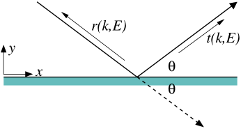
Figure 1: Geometry of specular and Andreev reflection from the boundary.

We now investigate the effect of a boundary. Suppose, as shown in figure 1, that there is a wall at $y=0$, with the fluid lying above it. We seek solutions to the Bogoliubov equation in the form

$$\Psi=C_{+}\left[\matrix{a_{+}(y)\cr b_{+}(y)}\right]e^{ik_{f}x\cos\theta+ik_{f}y\sin\theta}-C_{-}\left[\matrix{a_{-}(y)\cr b_{-}(y)}\right]e^{ik_{f}x\cos\theta-ik_{f}y\sin\theta},$$ (14)

where now $a_{\pm}$ and $b_{\pm}$ are allowed to vary with $y$ — but slowly on the scale of $k_{f}$. We impose the boundary condition that $\Psi=0$ at $y=0$. The resultant equations for $a_{\pm}$ and $b_{\pm}$ coincide with those derived in the appendix for the solutions of a one-dimensional Dirac hamiltonian. The vanishing of the wavefunction at the wall becomes (because of the minus sign before $C_{-}$) the continuity of the Dirac wavefunction at $x=0$. The incoming particle therefore sees the reflecting boundary only as an abrupt change in the phase of the orbital part of the order parameter, which jumps from $-\theta$ to $+\theta$. The transmitted Dirac wave with amplitude $t(k,E)$ corresponds to those particles that have been specularly reflected at boundary, and the backscattered Dirac wave with amplitude $r(k,E)$ corresponds to those particles that have been Andreev reflected, and so retrace their path. The only significant differences between the two dimensional geometry and the one-dimensional problem solved in the appendix are that the co-ordinate “$x$” in the appendix is the distance along the classical trajectory, and that there we have set the Fermi velocity $v_{f}$ to unity. Thus, expressions appearing in the appendix, such as $e^{-\kappa|x|}$ must here be replaced by $e^{-\kappa|y|/(v_{f}\sin(\theta))}$.

On making the appropriate translations from the results in the appendix, we find that we have a bound state

$$\chi_{0}(k_{x})=\sqrt{{\Delta\over 2v_{f}}}e^{ik_{f}x\cos\theta}\sin(k_{f}y\sin\theta)e^{-\Delta y/v_{f}}\left[\matrix{1\cr 1}\right]$$ (15)

with energy

$$E_{0}(k_{x})=-\Delta\cos\theta=-\Delta(k_{x}/k_{f}).$$ (16)

The associated edge excitations are therefore chiral, or Weyl, fermions, having group velocity $\partial E/\partial k_{x}$ only in the $-\hat{\bf x}$ direction. This motion is in the opposite sense to the anticlockwise orbital angular momentum of the Cooper pairs.

These edge modes have a topological character. All that is required for them to exist is that the fluid density fall to zero at the boundary [2]. Indeed the edge-mode spectrum (16) for our rigid wall boundary coincides with that obtained by Read and Green [1] in the opposite extreme of a very soft wall.

The contribution of the edge-modes to the field operator $\hat{\Psi}$ is

$$\sum_{k_{x}}\hat{a}_{0,k_{x}}\chi_{0,k_{x}}(x),$$ (17)

and, in order for the upper and lower components to reconstruct $\hat{\psi}$ and $\hat{\psi}^{\dagger}$ respectively, we must have $\hat{a}_{0,k_{x}}=\hat{a}_{0,-k_{x}}^{\dagger}$. The edge-mode field

$$\hat{\Psi}_{0}(x)=\int_{-k_{f}}^{k_{f}}{dk\over 2\pi}\hat{a}_{0,k_{x}}\chi_{0,k_{x}}(x)$$ (18)

is therefore real, $\hat{\Psi}_{0}(x)=\hat{\Psi}_{0}^{\dagger}(x)$, or Majorana.

It is difficult for anything interact with a Majorana-Weyl particle. A Weyl particle can interact only via currents, and no current operator can be constructed from a single Majorana field. In our superfluid there are, however, two Majorana-Weyl fields: one for spin up and one for spin down. Out of these two real fields we can construct one complex Weyl field

$$\hat{\Psi}_{c} = {1\over\sqrt{2}}(\hat{\Psi}_{\uparrow 0}+i\hat{\Psi}_{\downarrow 0}),$$

$$\hat{\Psi}^{\dagger}_{c} = {1\over\sqrt{2}}(\hat{\Psi}_{\uparrow 0}-i\hat{\Psi}_{\downarrow 0}),$$ (19)

and from this we can construct a unique $U(1)$ current operator

$$\hat{\Psi}^{\dagger}_{c}\hat{\Psi}_{c}={i\over 2}\left(\hat{\Psi}_{\uparrow 0}\hat{\Psi}_{\downarrow 0}-\hat{\Psi}_{\downarrow 0}\hat{\Psi}_{\uparrow 0}\right)={1\over 2}\hat{\Psi}_{0}\sigma_{2}\hat{\Psi}_{0}.$$ (20)

The edge modes may therefore interact with the $\sigma_{2}$ component of a spin-coupled gauge field.

III.1.2 Boundary current

The doubling of the number of degrees of freedom in the Bogoliubov formalism requires us, when computing ground-state expectation values of an operator, to sum the contributions of all occupied (negative energy) states, but then divide by two to prevent over-counting — this division by two being equivalent to imposing the reality condition on the $\hat{a}_{E,{\bf k}}$. The mass current carried by the state

$$\Psi=\left[\matrix{a\cr b}\right]e^{ik_{f}x\cos\theta+ik_{f}y\sin\theta},$$ (21)

where $a$, $b$ are slowly varying compared to $k_{f}$ is therefore

$${\bf j}={1\over 2}(|a|^{2}+|b|^{2})(k_{f}\cos\theta,k_{f}\sin\theta).$$ (22)

The edge modes with $k_{x}>0$ have negative energy, and so are occupied in the ground state where they make a positive contribution to the boundary momentum density. For a Galilean invariant system, the momentum density is also the mass current. The edge modes therefore tend to produce a boundary current that flows in the same sense as the Cooper-pair rotation. The bound states, however, are not the only contribution to this boundary current. The balance is provided by the phase-shifted scattering states, which (as they do the theory of fractional charge [23, 24]) partially cancel the contribution of a bound state when it has negative energy and is occupied, and partially make up for the absence of its contribution when it has positive energy and is unoccupied.

The current in the direction perpendicular to the wall will cancel between the incoming and outgoing waves, but the $\hat{\bf x}$ components will add. Using the results from the appendix, we find that the net mass-current running near the boundary is (for a single spin component)

$$\int_{0}^{\infty}j_{x}dy = \int_{0}^{1}{d(k_{f}\cos\theta)\over 2\pi}\left({\theta\over 2\pi}\right)k_{f}\cos\theta+\int_{-1}^{0}{d(k_{f}\cos\theta)\over 2\pi}\left({\theta\over 2\pi}-{1\over 2}\right)k_{f}\cos\theta$$ (23)

$$= 2\int_{0}^{1}{d(k_{f}\cos\theta)\over 2\pi}{\theta\over 2\pi}k_{f}\cos\theta$$

$$= {k_{f}^{2}\over 16\pi}={1\over 4}\rho,$$

where $\rho=k_{f}^{2}/4\pi$ is the number density per spin component. If this current flows at the edge of a disc-shaped region of radius $R$, it provides angular momentum

$${\bf L}=2\pi R^{2}\left({\rho\over 4}\right)\hat{\bf z}={N\over 2}\hat{\bf z}.$$ (24)

This result agrees with that of Kita [7], and Volovik [20] and is exactly the angular momentum we would expect of a fluid of tightly bound Cooper pairs, each pair having orbital angular momentum of $\hbar\hat{\bf z}$. That the same result holds in the weak coupling limit, where only the particles near the Fermi-surface are affected by the pairing, is more surprising, and it is often referred to as the “angular momentum paradox” (see Kita [7] for a recent review of this).

Our result for the boundary current differs from that of Furusaki et al. [19], because they consider only the the bound state contributions. The boundary current arising from the bound states alone is (again for a single spin component)

$${1\over 2}\int_{0}^{1}{d(k_{f}\cos\theta)\over 2\pi}k_{f}\cos\theta={k_{f}^{2}\over 8\pi}={\epsilon_{f}m\over 4\pi}.$$ (25)

After multiplying by two to take into account the two spin components, this coincides with equation (2.8) in Furusaki et al. [19], and differs from the actual persistent boundary current by a factor of two.

We have computed the boundary current only in the weak coupling limit, but the result that it precisely accounts for the $\hbar$-per-pair angular momentum should remain valid even as the coupling is increased. This is because, provided the ground state evolves adiabatically, its total angular momentum cannot change as we alter parameters in the Hamiltonian. Adiabatic evolution may fail if there is spectral flow, and such flow does occur and change the angular momentum when we compute the angular momentum of some vortex configurations in bulk ³He-A [21], and also when we consider the dynamical intrinsic angular momentum density [22], but in the present case spectral flow can only occur through the gapless edge states and the $E_{0}(k_{x})=-E_{0}(-k_{x})$ Majorana symmetry prevents the spectrum moving en-masse with respect to the chemical potential. For the same reason, the total boundary current should also not be affected by local deviations of the order parameter away from its bulk form. The “fractional charge” interpretation [23, 24, 25] of the current ensures this, because the total fractional charge depends only on the asymptotics of the order parameter, and is unaffected by local variations.

III.2 Disc geometry

When the fluid has disc geometry it is convenient to use polar coordinates $r$, $\theta$, and to work with angular momentum eigenstates $\propto e^{il\theta}$. For example, we have

$$-\nabla^{2}J_{l}(kr)e^{il\theta}=k^{2}J_{l}(kr)e^{il\theta},$$ (26)

where $J_{l}(kr)$ is a Bessel function. In polar coordinates, the orbital part of the gap operator $\hat{P}=-(\partial_{x}+i\partial_{y})$ becomes

$$\hat{P}=-e^{i\theta}\left({\partial\over\partial r}+{i\over r}{\partial\over\partial\theta}\right),$$ (27)

and has a particularly simple action on the Laplace eigenfunctions:

$$\hat{P}e^{il\theta}J_{l}(kr)=ke^{i(l+1)\theta}J_{l+1}(kr).$$ (28)

The adjoint operator

$$\hat{P}^{\dagger}=-\left(-{1\over r}{\partial\over\partial r}r+{i\over r}{\partial\over\partial\theta}\right)e^{-i\theta}=-e^{i\theta}\left(-{\partial\over\partial r}+{i\over r}{\partial\over\partial\theta}\right),$$ (29)

similarly acts to reduce the angular momentum eigenvalue

$$\hat{P}^{\dagger}e^{il\theta}J_{l}(kr)=ke^{i(l-1)\theta}J_{l-1}(kr).$$ (30)

We look for eigenstates in the form

$$\psi=\left[\matrix{aJ_{l+1}(kr)e^{i(l+1)\theta}\cr bJ_{l}(kr)e^{il\theta}}\right].$$ (31)

The Bogoliubov equation, ${\hat{H}}\Psi=E\Psi$, then reduces to

$$\left[\matrix{\epsilon(k)&(k/k_{f})\Delta\cr(k/k_{f})\Delta&-\epsilon(k)}\right]\left[\matrix{a\cr b}\right]=E\left[\matrix{a\cr b}\right].$$ (32)

The eigenstates are therefore

$$\Psi_{E,l}(r,\theta)={1\over 2\sqrt{E(E+\Delta)}}\left[\matrix{(E+\epsilon+\Delta)e^{i(l+1)\theta}J_{l+1}(kr)\cr(E-\epsilon+\Delta)e^{il\theta}J_{l}(kr)}\right],$$ (33)

where the energy eigenvalue is

$$E=+\sqrt{\epsilon^{2}(k)+(k/k_{f})^{2}\Delta^{2}},$$ (34)

and

$$\Psi_{-|E|,l}(r,\theta)={1\over 2\sqrt{|E|(|E|-\Delta)}}\left[\matrix{(|E|-\Delta-\epsilon)e^{i(l+1)\theta}J_{l+1}(kr)\cr(|E|-\Delta+\epsilon|E|)e^{il\theta}J_{l}(kr)}\right],$$ (35)

with energy

$$E=-\sqrt{\epsilon^{2}(k)+(k/k_{f})^{2}\Delta^{2}}.$$ (36)

As before, we are interested in momenta near the Fermi-surface where the energy can be approximated by

$$E=\pm\sqrt{v_{f}^{2}(k-k_{f})^{2}+\Delta^{2}}.$$ (37)

When we confine the fluid by imposing rigid wall boundary conditions at $r=R$, the eigenstates will be a linear combination

$$\Psi_{l}=C_{+}\left[\matrix{a_{+}J_{l+1}(k_{+}r)e^{i(l+1)\theta}\cr b_{+}J_{l}(k_{+}r)e^{il\theta}}\right]-C_{-}\left[\matrix{a_{-}J_{l+1}(k_{-}r)e^{i(l+1)\theta}\cr b_{-}J_{l}(k_{-}r)e^{il\theta}}\right],$$ (38)

of unconfined states with slightly different momentum $k_{\pm}=k_{f}\pm k$, but a common energy

$$E=\pm\sqrt{v_{f}^{2}k^{2}+\Delta^{2}}.$$ (39)

The coefficients $a_{\pm}$ and $b_{\pm}$ are given by

$$\left[\matrix{a_{\pm}\cr b_{+}}\right]=\left[\matrix{E\pm v_{f}k+\Delta\cr E\mp v_{f}k+\Delta}\right].$$ (40)

To examine the consequences of the condition that $\Psi=0$ at $r=R$ we use the WKB approximation for the Bessel function

$$J_{l}(kr)\approx\sqrt{{2\over\pi kx(r)}}\sin(kx(r)-l\theta(r)-\pi/4),\qquad r\gg b.$$ (41)

Here $x(r)$ and $\theta(r)$ are functions of $r$, defined in terms of the semi-classical impact parameter, $b=l/k$, by $x=r\sin\theta$ and $b=r\cos\theta$. As illustrated in figure 2, the parameter $x$ has the physical interpretation of being the distance along the straight-line semi-classical trajectory. This approximation is quite accurate once $r$ exceeds $b$ by more than a few percent, and is therefore reliable except for a few large values of $l$ which correspond to classical trajectories grazing the boundary. Using the WKB approximation and the explicit form of the coefficients $a_{\pm}$ and $b_{\pm}$ we we end up with exactly the same equations for the bound state and $S$ matrix that we found in the planar boundary case.

Figure 2: The geometry of the WKB approximation to the Bessel function.

There is some advantage to working with a circular container, however. With a finite length boundary, the set of edge modes becomes discrete — being labeled by the integer $l$. The angle $\theta$ between the semi-classical trajectory and the boundary is $\theta(R)$, and $l=k_{f}R\cos\theta(R)$. In terms of $l$, therefore, the bound state has energy

$$E_{0}(l)\approx-\left({l\over l_{{max}}}\right)\Delta,$$ (42)

where $l_{{max}}=k_{f}R$. The WKB approximation is not quite good quite good enough to distinguish between $l$ and $l+{1\over 2}$ in this expression, but on general grounds we know that if $(u,v)^{T}$ is an eigenstate of the Bogoliubov Hamiltonian with energy $E$, then $(v^{*},u^{*})^{T}$ is also an eigenstate with energy $-E$. Under this transformation $\Psi_{l}\to\Psi_{-(l+1)}$, and so the correct equation must be

$$E_{0}(l)=-\left({l+1/2\over l_{{max}}}\right)\Delta.$$ (43)

There is therefore no exact zero-mode. If, however, the bulk fluid were to contain an odd number of vortices, and thus the phase of the order parameter wind an odd number of times as we encircle the boundary, then the $l$’s appearing in the upper and lower components of $\Psi$ would differ by an even number. In this case there will be a zero energy edge state. Since each vortex has a zero-mode in its core [4], there will be an unpaired zero-energy core mode which can pair with the zero-energy edge state and so preserve the even dimension of the total Bogoliubov-particle Hilbert space.

This dependence of the edge-mode spectrum on the number of the bulk vortex excitations is reminiscent of what happens in the quantum Hall effect. There the Hilbert space sector of the edge conformal field theory also depends on the number and type of vortex quasi-particles that are present in the bulk.

IV Effective actions

We now discuss the effective action governing the low-energy dynamics of the superfluid. We will obtain the action by examining the response of the fluid to external gauge fields that couple to the particle number and spin of the fluid.

IV.1 Particle-number symmetry

We begin by gauging the $U(1)$ symmetry corresponding to particle-number conservation. We will again hold the ${\bf d}$ vector fixed in the $\hat{\bf y}$ direction so we can treat each spin component separately. We minimally couple the particle-number current to an Abelian gauge field $(A_{0},{\bf A})$, where $A_{0}$ is the time component and ${\bf A}\equiv(A_{1},A_{2})$ are the in-plane components of the externally imposed field. This requires the replacement

$$i\partial_{t}-{\hat{H}}\to i\partial_{t}-{\hat{H}}(A,\Phi)$$ (44)

where

$${\hat{H}}(A,\Phi)=\left[\matrix{-{1\over 2m}(\nabla-i{\bf A})^{2}-A_{0},&i\left({\Delta\over k_{f}}\right)e^{i\Phi/2}\hat{P}e^{i\Phi/2}\cr-i\left({\Delta\over k_{f}}\right)e^{-i\Phi/2}\hat{P}^{\dagger}e^{-i\Phi/2},&{1\over 2m}(\nabla+i{\bf A})^{2}+A_{0}}\right].$$ (45)

The resulting action

$$S(A,\Phi,\Psi,\Psi^{\dagger})=\int d^{2}x\,dt\,\Psi^{\dagger}\left(i\partial_{t}-{\hat{H}}(A,\Phi)\right)\Psi$$ (46)

is then invariant under the local gauge transformation

$$\left[\matrix{\psi\cr\psi^{\dagger}}\right]\to\left[\matrix{e^{i\phi}\psi,\cr e^{-i\phi}\psi^{\dagger}}\right],$$ (47)

provided we simultaneously transform

$$\Phi \to \Phi+2\phi,$$

$${\bf A} \to {\bf A}+\nabla\phi,$$

$$A_{0} \to A_{0}+\partial_{t}\phi.$$ (48)

Because the Grassmann measure in the path integral is left invariant by the transformation (47), the effective action

$$iS_{\rm eff}^{\rm num}(A,\Phi) = \ln\left\{\int d[\Psi]d[\Psi^{\dagger}]\exp[iS(A,\Phi,\Psi,\Psi^{\dagger})]\right\}$$ (49)

$$= {1\over 2}\ln{\rm Det\,}(i\partial_{t}-{\hat{H}}(A,\Phi))$$

will be invariant under the transformation (48). If we compute (49) to second order in the gauge field and its gradients, we find [8, 18], for a single spin component,

$$S_{\rm eff}^{\rm num}(A,\Phi) = \int d^{2}xdt\left\{{\rho_{0}\over 2m}\left[{1\over c_{s}^{2}}\left({\partial\Phi/2\over\partial t}-A_{0}\right)^{2}-\left(\nabla\Phi/2-{\bf A}\right)^{2}\right]\right.$$

$$\quad\left.-\sigma_{xy}\left({\partial\Phi/2\over\partial t}-A_{0}\right)\left(\nabla\times{\bf A}\right)_{z}-\rho_{0}\left({\partial\Phi/2\over\partial t}-A_{0}\right)\right\}.$$

Here, $\sigma_{xy}={1\over 8\pi}$, the parameter $c_{s}$ is the speed of sound, and $\rho_{0}$ the equilibrium number density. The coefficient $\sigma_{xy}$ is topologically stable, but the other quantities depend on the details of the fluid [8]. For a 2+1 dimensional Galilean invariant system of particles with mass $m$ we have $\rho_{0}={m\over 2\pi}\epsilon_{f}$ and $c_{s}=v_{f}/2$. The action (LABEL:EQ:Abelian_action) is manifestly invariant under the transformation (48).

The term with coefficient $\sigma_{xy}$ contains a Chern-Simons-like part

$$\sigma_{xy}\int d^{2}x\,dt\epsilon_{0ij}A_{0}\,\partial_{i}A_{j}.$$ (51)

This is not a complete Chern-Simons action, however, because there is no $\epsilon_{i0j}A_{i}\,\partial_{t}A_{j}$ term. It does, nonetheless, imply the existence of a Hall-like response to the external field. We find for the particle-number current

$${\bf j}_{\,\rm num} \equiv {\delta S_{\rm eff}^{\rm num}\over\delta\bf A}={\rho_{0}\over m}\left(\nabla\Phi/2-e{\bf A})\right)+\sigma_{xy}({\hat{\bf z}}\times\nabla)\left({\partial\Phi/2\over\partial t}-A_{0}\right)$$ (52)

$$= \rho_{0}{\bf v}_{s}+\sigma_{xy}({\hat{\bf z}}\times\nabla)\left({\partial\Phi/2\over\partial t}-A_{0}\right).$$

Although the term with $\sigma_{xy}$ contains a gradient of $A_{0}$, it is not equal to $\sigma_{xy}({{\bf E}\times\hat{\bf z}})$, where ${\bf E}=\nabla A_{0}-\dot{\bf A}$, as it would be in the Hall effect. (Observe that $\nabla\dot{\Phi}/2$ cannot be $\dot{\bf A}$ in disguise, because the former is necessarily curl-free.) We note, however, that the combination $(\partial_{t}\Phi/2-A_{0})$ occurs in the the expression for the density

$$\rho\equiv{\delta S_{\rm eff}^{\rm num}\over\delta A_{0}}=\rho_{0}-{\rho_{0}\over mc_{s}^{2}}\left({\partial\Phi/2\over\partial t}-A_{0}\right)+\sigma_{xy}\nabla\times{\bf A}.$$ (53)

Consequently, it seems preferable to write

$${\bf j}_{\,\rm num}=\rho_{0}{\bf v}_{s}-{1\over 4m}({\hat{\bf z}}\times\nabla)(\rho-\sigma_{xy}B_{z}),$$ (54)

where $B_{z}=(\nabla\times{\bf A})_{z}$, and so recognize that the “Hall” current depends on the external field primarily through its effect in modifying the density. The natural analogy is then with the bound current ${\bf j}_{\,\rm bound}=\nabla\times{\bf M}$ in a magnet with varying magnetization ${\bf M}$. In the superfluid, the magnetic-moment density ${\bf M}$ is replaced by the intrinsic angular momentum density ${1\over 2}\hbar(\rho-\sigma_{xy}B_{z})\hat{\bf z}$. The $\sigma_{xy}B_{z}$ correction is presumably present because a diamagnetic response to the external field will reduce the kinetic angular momentum of a Cooper pair even while leaving its canonical angular momentum fixed at $\hbar$. In the absence of an external $B_{z}$ field, we therefore have a mass flux

$${\bf j}=m\,{\bf j}_{\,\rm num}={1\over 4}\nabla\times{\rho\hat{\bf z}},$$ (55)

and this is a planar analogue of the Mermin-Muzikar current [6]. When $\rho$ goes to zero slowly at a boundary we can use this Mermin-Muzikar expression to compute the equilibrium boundary-current. The resulting boundary momentum density coincides with that we computed for a rigid wall in section III, and again provides an $\hbar$-per-Cooper pair angular momentum. This agreement between the rigid-boundary calculation and the gradient expansion when expressed in terms of the density, coupled with the physical explanation in terms of the intrinsic angular momentum of the fluid, leads us to conjecture that the total mass-current is always proportional to the change in density, rather than to the external force that causes the change.

IV.2 Spin-rotation symmetry

The fields in

$$S=\int d^{2}xdt\left(\Psi^{\dagger}(i\partial_{t}-{\hat{H}})\Psi\right)$$ (56)

can also be coupled to an $SU(2)$ gauge field which acts on the spin indices. To do this we replace the derivatives in $S$ by covariant derivatives

$$\partial_{\mu}\to\partial_{\mu}+{\mathcal{A}}_{\mu},$$ (57)

where

$${\mathcal{A}}_{\mu}=i\sigma_{a}{\mathcal{A}}^{a}_{\mu}$$ (58)

is an externally imposed gauge field. Under a local gauge transformation the Fermi fields transform as

$$\Psi=\left[\matrix{\psi\cr\psi^{\dagger}}\right]\to\left[\matrix{U\psi\cr U^{*}\psi^{\dagger}}\right],\quad\Psi^{\dagger}=\left[\matrix{\psi^{\dagger},&\psi}\right]\to\left[\matrix{\psi^{\dagger}U^{-1},&\psi U^{T}}\right],$$ (59)

where $U\in SU(2)$. The covariant derivatives transform as

$$\partial_{\mu}+{\mathcal{A}}_{\mu}\to U^{-1}(\partial_{\mu}+{\mathcal{A}}_{\mu})U=\partial_{\mu}+(U^{-1}{\mathcal{A}}_{\mu}U+U^{-1}\partial_{\mu}U).$$ (60)

When considering how the transformation act in the $-\hat{h}^{T}$ entry in ${\hat{H}}$, we need to recognize that derivative operators appearing there are the transpose $\partial_{\mu}^{T}=-\partial_{\mu}$ of those in $\hat{h}$, and so the covariant derivatives will be also be the transpose $\partial_{\mu}^{T}+{\mathcal{A}}_{\mu}^{T}=-\partial_{\mu}+{\mathcal{A}}_{\mu}^{T}$. Using $U^{*}=(U^{-1})^{T}=(U^{T})^{-1}$, we have

$$U^{T}(\partial_{\mu}^{T}+{\mathcal{A}}_{\mu}^{T})(U^{T})^{-1} = -\partial_{\mu}+U^{T}{\mathcal{A}}_{\mu}^{T}(U^{T})^{-1}-U^{T}(U^{T})^{-1}\partial_{\mu}U^{T}(U^{T})^{-1}$$ (61)

$$= -\partial_{\mu}+(U^{-1}{\mathcal{A}}_{\mu}U+U^{-1}\partial_{\mu}U)^{T}$$

$$= [\partial_{\mu}+(U^{-1}{\mathcal{A}}_{\mu}U+U^{-1}\partial_{\mu}U)]^{T},$$

and the the effect of the transformation is consistent for both entries:

$${\mathcal{A}}_{\mu}\to A_{\mu}^{U}\equiv U^{-1}{\mathcal{A}}_{\mu}U+U^{-1}\partial_{\mu}U.$$ (62)

Note that $({\mathcal{A}}^{U})^{V}={\mathcal{A}}^{UV}$. For the off diagonal terms we have

$$U^{-1}\hat{\Sigma}U^{*}=U^{-1}\left(i(\sigma\cdot{\bf d})\sigma_{2}\right)U^{*}=\left(iU^{-1}(\sigma\cdot{\bf d})U\sigma_{2}\right).$$ (63)

The net result is that the gauged action is invariant under the transformation (59), provided we simultaneously transform

$$({\bf d}\cdot\sigma) \to U(\sigma\cdot{\bf d})U^{-1}$$

$${\mathcal{A}}_{\mu} \to {\mathcal{A}}_{\mu}^{U^{-1}}=U{\mathcal{A}}_{\mu}U^{-1}+U\partial_{\mu}U^{-1}.$$ (64)

Following Volovik and Yakovenko [17], we now compute the effective action with the $\bf d$ vector fixed to lie in the $\hat{\bf y}$ direction, and find a Chern-Simons term

$$S_{\rm eff}^{\rm spin}({\bf d}=\hat{\bf y},{\mathcal{A}})={1\over 8\pi}\int{\rm tr\,}\left({\mathcal{A}}d{\mathcal{A}}+{2\over 3}{\mathcal{A}}^{3}\right).$$ (65)

Here we use differential-form notation in which ${\mathcal{A}}\equiv i\sigma_{a}{\mathcal{A}}^{a}_{\mu}dx^{\mu}$ is a matrix valued 1-form. For any compact simple gauge-group $G$, the Chern-Simons action is defined to be

$$C({\mathcal{A}})={1\over 4\pi}\int_{\Omega}{\rm tr\,}\left({\mathcal{A}}d{\mathcal{A}}+{2\over 3}{\mathcal{A}}^{3}\right),$$ (66)

where ${\mathcal{A}}\equiv i\lambda_{a}{\mathcal{A}}^{a}_{\mu}dx^{\mu}$ is a ${\rm Lie\,}(G)$-algebra-valued 1-form, and, as is customary, we normalize the trace and the Hermitian generators $\lambda_{a}$ by ${\rm tr\,}(\lambda_{a}\lambda_{b})=2\delta_{ab}$. When such a term is to appear in a functional integral,

$$Z=\int d[{\mathcal{A}}]e^{ikC({\mathcal{A}})},$$ (67)

then coefficient $k$ must be quantized. This is because under a gauge transformation

$${\mathcal{A}}\to{\mathcal{A}}^{g}\equiv g^{-1}{\mathcal{A}}g+g^{-1}dg$$ (68)

we have

$$C({\mathcal{A}})\to C({\mathcal{A}}^{g})=C({\mathcal{A}})-{1\over 12\pi}\int_{\Omega}{\rm tr\,}\left[(g^{-1}dg)^{3}\right]-{1\over 4\pi}\int_{\partial\Omega}{\rm tr\,}(dgg^{-1}{\mathcal{A}}).$$ (69)

Here, $\Omega$ is the region occupied by the fluid and $\partial\Omega$ its boundary. The last term is zero when $\Omega$ is closed manifold, or if we restrict the gauge transformation to those constant on the boundary. The second term,

$${\mathcal{W}}(g)={1\over 12\pi}\int_{\Omega}{\rm tr\,}\left[(g^{-1}dg)^{3}\right],$$ (70)

has no reason to vanish, however. It is the pull-back to $\Omega$ of an element of, $H^{3}_{DR}(G,{\bf Z})$, the third de-Rham cohomology group of $G$. It can be non-zero whenever the gauge transformation $g(x)$ maps $\Omega$ into a homologically non-trivial $3$-manifold in $G$. In particular, when $\Omega$ is $S^{3}$ and the group $G$ is $SU(2)$, then

$${1\over 12\pi}\int_{\Omega}{\rm tr\,}\left[(g^{-1}dg)^{3}\right]=2\pi n,$$ (71)

where $n$ is the degree of the map from $S^{3}\to SU(2)\simeq S^{3}$. In this case $k$ has to be an integer so that the gauge ambiguity in $C({\mathcal{A}})$ is $2\pi kn$ and $\exp(ikC({\mathcal{A}}))$ is well-defined.

The Chern-Simons action found by Volovik and Yakovenko has a coefficient corresponding to $k=1/2$, and so violates the quantization condition on $k$. It cannot be gauge invariant on its own. The complete effective action will be gauge invariant, of course, but we must include additional degrees of freedom to make this manifest. One of these is the direction of the vector $\bf d$, which we must therefore allow to vary. We parameterize $\bf d$ in terms of a group element $V\in SU(2)$ by setting

$$({\bf d}\cdot\sigma)=V\sigma_{2}V^{-1}.$$ (72)

Then,

$$S_{\rm eff}^{\rm spin}({\bf d},{\mathcal{A}})=S_{\rm eff}^{\rm spin}(\hat{\bf y},{\mathcal{A}}^{V})={1\over 2}C({\mathcal{A}}^{V}).$$ (73)

This expression is clearly invariant under the simultaneous replacement ${\mathcal{A}}\to{\mathcal{A}}^{U}$ and $V\to U^{-1}V$. This is good, but not perfect. The problem is that $V$ is not unique. The vector ${\bf d}$ is more correctly paramaterized by elements of the coset $SU(2)/U(1)$, since we can replace $V$ by $Ve^{i\sigma_{2}\phi}$ without changing $\bf d$. This substitution does affect $C({\mathcal{A}}^{V})$, however. Compensating for the effects of $e^{i\sigma_{2}\phi}$ requires yet another degree of freedom. We will write this as $W=e^{i\sigma_{2}\chi}$. A completely gauge invariant action is then

$$S_{\rm eff}^{\rm spin}({\bf d},{\mathcal{A}},\chi)={1\over 2}C({\mathcal{A}}^{VW}).$$ (74)

This is manifestly invariant under the simultaneous replacement

$${\mathcal{A}}\to{\mathcal{A}}^{U},$$

$$V\to U^{-1}Ve^{i\sigma_{2}\phi},$$

$$\chi\to\chi-\phi.$$ (75)

What is the physical interpretation of this extra field $\chi$? This question is easiest to answer if we set $V=I$ on the boundary, so that ${\bf d}=\hat{\bf y}$ there. Then, using the Polyakov-Wiegmann identity (69) we can write

$$S_{\rm eff}^{\rm spin}({\bf d},{\mathcal{A}},\chi) = {1\over 2}C({\mathcal{A}}^{VW})={1\over 2}C(A)-{1\over 24\pi}\int_{\Omega}{\rm tr\,}\left[(V^{-1}dV)^{3}\right]$$ (76)

$$\qquad-{1\over 8\pi}\int_{\partial\Omega}{\rm tr\,}\left\{dWW^{-1}{\mathcal{A}}\right\}.$$

The second term

$${1\over 2}{\mathcal{W}}(V)={1\over 24\pi}\int_{\Omega}{\rm tr\,}\left[(V^{-1}dV)^{3}\right],$$ (77)

is precisely the Hopf index found by Volovik and Yakovenko. On a closed manifold, or when ${\bf d}$ is fixed at the boundary, it is equal to $n\pi$ where $n$ labels the homotopy class of the map ${\bf d}:S^{3}\to S^{2}$. The Berry phase provided by this term makes a skyrmion soliton in the ${\bf d}$ field into a fermion. The third term,

$$-{1\over 8\pi}\int_{\partial\Omega}{\rm tr\,}\left\{dWW^{-1}{\mathcal{A}}\right\},$$ (78)

is equal to

$$-{i\over 8\pi}\int_{\partial\Omega}{\rm tr\,}\left\{d\chi\sigma_{2}{\mathcal{A}}\right\}={1\over 4\pi}\int dxdt\left\{{\mathcal{A}}_{0}^{2}\partial_{x}\chi-{\mathcal{A}}_{x}^{2}\partial_{t}\chi\right\},$$ (79)

and represents the coupling of the $\chi$ field current to the $\sigma_{2}$ component of ${\mathcal{A}}$. This interaction takes place only on the boundary, which we have taken to be the $x$ axis as in section III.1. This suggests that the $\chi$ field is the bosonized form of the complex Weyl fermion $\Psi_{c}$ that we constructed out of the two Majorana-Weyl edge modes in section III.1. As we noted there, $\Psi_{c}$ naturally couples to the $\sigma_{2}$ component of ${\mathcal{A}}$.

Gauge invariance tells us that the edge-modes must exist, but it does not determine their dynamics. We can, however, add a manifestly gauge invariant boundary term that ensures that the $\chi$ field propagates unidirectionallly at speed $c=-\Delta/k_{f}$. This term is [11]

$$-{c\over 8\pi}\int dxdt\,{\rm tr\,}\left\{[W^{-1}(\partial_{x}+{\mathcal{A}}_{x})W][W^{-1}(\partial_{x}+c^{-1}\partial_{t}+{\mathcal{A}}_{x}+c^{-1}{\mathcal{A}}_{t})W]\right\}.$$ (80)

Including it, and writing $W=e^{i\sigma_{2}\chi}$, the effective action becomes

$$S_{\rm eff}^{\rm spin}({\bf d},{\mathcal{A}},\chi) = {1\over 2}C({\mathcal{A}})-{1\over 2}{\mathcal{W}}(V)+{c\over 4\pi}\int dxdt\,\left\{\partial_{x}\chi[(c^{-1}\partial_{t}+\partial_{x})\chi]\right\}$$

$$+{1\over 2\pi}\int dxdt\left\{(c{\mathcal{A}}^{2}_{x}+{\mathcal{A}}^{2}_{t})\partial_{x}\chi\right\}-{1\over 8\pi}\int dxdt\,{\rm tr\,}\left\{(c{\mathcal{A}}_{x}+{\mathcal{A}}_{t}){\mathcal{A}}_{x}\right\}.$$

The terms containing $\chi$ now constitute the action for a chiral boson interacting with the appropriate chiral component of the gauge field. The entire expression is invariant under gauge transformations $U$ which reduce to the form $e^{i\sigma_{2}\phi}$ on the boundary, and so maintain ${\bf d}=\hat{\bf y}$ there. We note that the factor of $1/2$ in the “level” $k$ is compensated for by a factor $2$ coming from ${\rm tr\,}(\sigma_{2}^{2})=2$, so as to give the correct scale for a chiral boson representing a Weyl fermion.

Since the action of the $U(1)$ and $SU(2)$ gauge groups commute with one another, the complete gauge invariant effective action containing all the low-energy degrees of freedom is the sum

$$S^{\rm tot}_{\rm eff}(A,\Phi,{\bf d},{\mathcal{A}},\chi)=2S^{\rm num}_{\rm eff}(A,\Phi)+S^{\rm spin}_{\rm eff}({\bf d},{\mathcal{A}},\chi).$$ (82)

Here the “2” in front of $S^{\rm num}_{\rm eff}$ comes from the two spin components.

V Conclusions

We have investigated the gauge invariance of the low-energy effective action for a $2+1$ dimensional chiral superfluid coupled to external gauge fields. When the order parameter completely breaks the gauge group, as in the case of Abelian particle-number symmetry, the effective action becomes manifestly gauge invariant as soon as we include the bulk Goldstone modes among the dynamical fields. When the gauge symmetry is not completely broken, as in the case of spin-rotation symmetry, we found that additional, non-Goldstone, degrees of freedom were required for manifest gauge invariance. These were identified as being the spin-up and spin-down Majorona-Weyl edge fermions, which could be combined to produce a current that soaks up the remaining gauge dependence.

The consequences of the effective actions for spin and particle-number currents also differ. The former has a true spin-Hall effect, with a dissipationless spin current proportional the spin “electric” field. The latter, we have argued, has only a “mock” Hall effect, the induced current being proportional to the change in density, and not to the external field causing the change.

VI Acknowledgments

This work was supported by the National Science Foundation under grant NSF-DMR-01-32990. MS would like to thank Eduardo Fradkin, Rinat Kedem and Eddy Ardonne for useful conversations, and Grisha Volovik for a valuable e-mail exchange.

Appendix A Dirac equation

The twisted-mass Dirac equation that results from our two-dimensional problem is a standard illustration of the theory of fractional charge [23]. We review it here so as to make clear the contribution of the extended scattering states to the boundary current.

We consider the one-dimensional Dirac Hamiltonian

$${\hat{H}}=-i\tau_{3}\partial_{x}+\Delta\tau_{1}e^{-i\tau_{3}\phi(x)}=\left[\matrix{-i\partial_{x}&\Delta e^{i\phi(x)}\cr\Delta e^{-i\phi(x)}&i\partial_{x}}\right],$$ (83)

where $\Delta$ is a constant.

We will compute the extra particle number that is accumulated in the vicinity of $x=0$ when $\phi$ is discontinuous, jumping abruptly from $\phi=\phi_{L}$ when $x<0$ to $\phi=\phi_{R}$ when $x>0$. Suppose the eigenstates of ${\hat{H}}$ are $\chi_{n}$ with energy $E_{n}$. The ground-state number density is

$${\langle\psi^{\dagger}\psi(x)\rangle}=\sum|\chi_{n}(x)|^{2},$$ (84)

where the sum is over occupied states, i.e. those with $E_{n}<0$. Because the sum of $|\chi_{n}|^{2}$ over all states is independent of $\phi$ by completeness, we can equally well write

$${\langle\psi^{\dagger}\psi(x)\rangle}=\hbox{const.}-\sum_{E_{n}>0}|\chi_{n}(x)|^{2},$$ (85)

and this form is slightly more convenient. We will show that

$$Q=\int{\langle\psi^{\dagger}\psi(x)\rangle}dx = {1\over 2\pi}(\phi_{R}-\phi_{L}),\quad 0<(\phi_{R}-\phi_{L})<\pi,$$ (86)

$$= {1\over 2\pi}(\phi_{R}-\phi_{L})-1,\quad\pi<(\phi_{R}-\phi_{L})<2\pi.$$

When $\phi$ is constant we have a continuum of positive and negative energy eigenfunctions

$$\psi^{\phi}_{k,E}=e^{i\sigma_{3}\phi/2}{1\over 2\sqrt{E(E+\Delta)}}\left[\matrix{E+k+\Delta\cr E-k+\Delta}\right]e^{ikx},$$ (87)

where $E(k)=\pm\sqrt{k^{2}+\Delta^{2}}$. With the discontinuity present, we will have scattering solutions

$$\psi = a_{L}^{(in)}\psi^{\phi_{L}}_{k,E}+a_{L}^{(out)}\psi^{\phi_{L}}_{-k,E},\quad x<0,$$

$$= a_{R}^{(in)}\psi^{\phi_{R}}_{-k,E}+a_{R}^{(out)}\psi^{\phi_{R}}_{k,E},\quad x>0.$$

The function $\psi$ must be continuous at $x=0$, and from this condition we obtain the $S$-matrix relation

$$\left[\matrix{a_{L}^{(out)}\cr a_{R}^{(out)}}\right]=\left[\matrix{t&r\cr r&t}\right]\left[\matrix{a_{R}^{(in)}\cr a_{L}^{(in)}}\right],$$ (88)

where

$$t(k,E) = {1\over\cos(\Phi/2)-(iE/k)\sin(\Phi/2)},$$

$$r(k,E) = {i(\Delta/k)\sin(\Phi/2)\over\cos(\Phi/2)-(iE/k)\sin(\Phi/2)}.$$ (89)

Here $\Phi$ is shorthand for $\phi_{L}-\phi_{R}$.

In addition to the continuum states there is also a single bound state

$$\psi_{0} \propto e^{i\sigma_{3}\phi_{R}/2}\left[\matrix{E_{0}+i\kappa+\Delta\cr E_{0}-i\kappa+\Delta}\right]e^{-\kappa x},\quad x>0,$$

$$\propto e^{i\sigma_{3}\phi_{L}/2}\left[\matrix{E_{0}-i\kappa+\Delta\cr E_{0}+i\kappa+\Delta}\right]e^{\kappa x}.\quad x<0.$$

The bound-state energy $E_{0}$ is also determined by continuity at $x=0$, which requires

$$E_{0} = \Delta\cos(\Phi/2),$$

$$\kappa = \Delta\sin(\Phi/2).$$

These formula are valid for $0<\Phi<2\pi$, where $\kappa$ is positive, and extend outside that interval with period $2\pi$. At $\Phi=0$ there is no bound state. As $\Phi$ increases, a bound state peels off the upper continuum. It passes through $E=0$ at $\Phi=\pi$, and merges with the lower continuum as $\Phi$ reaches $2\pi$. If $\Phi$ increases beyond $2\pi$, the process repeats with another state peeling off the upper continuum. Thus each $2\pi$ twist in $\Phi$ results in the net transfer of one state from the upper continuum to the lower.

Using the relation between $E_{0}$ and $\kappa$, we can write the normalized bound state as

$$\chi_{0}=\sqrt{{\kappa\over 2}}\left[\matrix{e^{i(\phi_{L}+\phi_{R})/4}\cr e^{-i(\phi_{L}+\phi_{R})/4}}\right]e^{-\kappa|x|}.$$ (90)

A complete set of states comprises $\chi_{0}$ together with

$$\chi_{k,E}=\left\{\matrix{\psi^{\phi_{L}}_{k,E}+r(k,E)\psi^{\phi_{L}}_{-k,E},&\quad x<0,\cr t(k,E)\psi^{\phi_{R}}_{k,E},&\quad x>0;}\right.\quad k>0.$$ (91)

$$\chi_{k,E}=\left\{\matrix{t(k,E)\psi^{\phi_{L}}_{k,E},&\quad x<0,\cr\psi^{\phi_{R}}_{k,E}+r(k,E)\psi^{\phi_{R}}_{-k,E},&\quad x>0}\right.\quad k<0$$ (92)

These basis states therefore switch from a wave incident from the left to one incident from the right as $k$ changes sign.

After using $|r|^{2}+|t|^{2}=1$, and the explicit form of the free eigenfunctions, we find

$$\sum_{E>\Delta}|\chi_{E}(x)|^{2}=\int_{-\infty}^{\infty}{dk\over 2\pi}|\chi_{E,k}(x)|^{2}=\hbox{const.}+\int_{-\infty}^{\infty}{dk\over 2\pi}r(k,E)\left({\Delta\over k}\right)e^{2ik|x|}.$$ (93)

Here the “const.” refers to terms that are independent of $\phi_{R,L}$. We can improve the numerical convergence of the integral by using Jordan’s lemma to push the contour of integration $\Gamma$ into the upper half plane, as shown in figure 3.

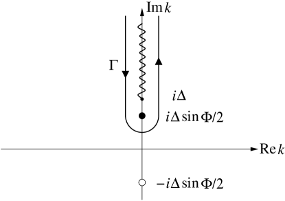
Figure 3: The contour $\Gamma$, showing the cut starting at $ik=\Delta$. When $0<\Phi<\pi$ there is pole at $k=i\Delta\sin\Phi/2$, and a pole on the second sheet at $k=-i\Delta\sin\Phi/2$.

We observe that the reflection coefficient has a cut running from $k=i\Delta$ to $i\infty$, and that for $0<\Phi<\pi$ there is a pole in the upper half plane at $k=i\Delta\sin\Phi/2$. At $\Phi=\pi$ the pole merges with the cut. For $\pi<\Phi<2\pi$ the pole is apparently returning towards the real axis again, but a more careful investigation shows that it is now on the second sheet, and no longer contributes. (At the same time a pole at $-i\Delta\sin\Phi/2$ has emerged onto the first sheet in the lower half plane. This is below the real axis, however, and also does not contribute.)

The integral in (93) then becomes

$$-\Delta\sin\Phi/2e^{-2\Delta|\sin\Phi/2||x|}+\int_{\Delta}^{\infty}{dk\over 2\pi}{\Delta^{2}\sin\Phi\over\kappa^{2}-\Delta^{2}\sin^{2}(\Phi/2)}{1\over\sqrt{\kappa^{2}-\Delta^{2}}}\kappa e^{-2\kappa|x|}.$$ (94)

The first term, the pole contribution, is only present if $0<\Phi<\pi$.

There does not seem to be a closed-form expression for the integral in (94), but if we first integrate over $x$ to get the total charge, we end up with an elementary integral

$$\int_{\Delta}^{\infty}{dk\over 2\pi}{\Delta^{2}\sin\Phi\over\kappa^{2}-\Delta^{2}\sin^{2}(\Phi/2)}{1\over\sqrt{\kappa^{2}-\Delta^{2}}}={\Phi\over 2\pi},\quad-\pi<\Phi<\pi.$$ (95)

This expression extends to a $2\pi$ periodic function of $\Phi$, and the integral is therefore discontinuous at odd multiples of $\pi$. After we include the pole contribution, which is discontinuous at all multiples of $\pi$, we find that the total continuum contribution is discontinuous only at $\Phi=0$ (mod $2\pi$). Thus

$$\int_{-\infty}^{\infty}{dk\over 2\pi}|\chi_{E,k}(x)|^{2}=\hbox{const.}+{\Phi\over 2\pi},\quad 0<\Phi<2\pi.$$ (96)

The discontinuity at $\Phi=0$ (mod $2\pi$) is due to the sudden loss of the bound state from the upper continuum. As the bound state makes its way to the lower continuum, the spectral weight in the upper continuum is gradually recovered.

We can now apply these results to compute

$$Q=\int\sum_{E_{n}<0}|\psi_{n}(x)|^{2}dx$$ (97)

We observe that our sum over the positive continuum is equal to minus the sum over the negative continuum together with the bound state. The bound state has negative energy, however, if $\pi<\Phi<2\pi$ (mod $2\pi$). If we are computing the ground state charge, and if $0<\Phi<\pi$ (mod $2\pi$), we should reduce the sum by unity. We also note that the constant in (96) is fixed by the requirement that the the accumulated charge be zero when $\phi_{L}=\phi_{R}$. Thus

$$Q = {1\over 2\pi}(\phi_{R}-\phi_{L}),\quad 0<(\phi_{R}-\phi_{L})<\pi,$$ (98)

$$= {1\over 2\pi}(\phi_{R}-\phi_{L})-1,\quad\pi<(\phi_{R}-\phi_{L})<2\pi.$$

This result repeats with $2\pi$ periodicity.

This expression for $Q$ is consistent with the basic result of Goldstone and Wilczek [23], that a total charge of

$$\int{1\over 2\pi}\partial_{x}\phi\,dx={1\over 2\pi}(\phi_{R}-\phi_{L})$$ (99)

is drawn into a region as the phase $\phi$ is slowly twisted. The difference between (98) and (99) arises because the latter does not keep track of individual particles that are lost to the reservoir when their energy exceeds the chemical potential.

In a superfluid the role of charge and current is interchanged. The fractional charge, multiplied by $k_{f}$ and divided by two, gives the momentum density, or equivalently, the mass current [25].

References

- [1] N. Read, D. Green, Phys. Rev. B 61, 10267 (2000).
- [2] G. E.Volovik, Pis’Ma V Zh. Eksp. Teor. Fiz. 66, 492-6 (1997) (English translation: JETP Letters (USA), 66, 522-7 (1997)).
- [3] G. Moore, N. Read, Nucl. Phys. B360, 362 (1991).
- [4] D. A. Ivanov, Phys. Rev. Lett, 86, 268-7 (2001).
- [5] K. Ishikawa, Prog. Theor. Phys. 57, 1836 (1977).
- [6] N. D. Mermin, P. Muzikar, Phys. Rev. B 21 980, (1980).
- [7] T. Kita, J. Phys. Soc. Japan, 67, 216-24 (1998).
- [8] G. E. Volovik, Phys. Scr. 38 321 (1988); Zh. Eksp. Teor. Fiz. 94, 123 (1988) (English translation: Soviet Physics (JETP) 67 1804-11 (1988)).
- [9] T. M. Rice, M. Sigrist, J. Phys, Condens. Matter 7, l643 (1995).
- [10] G. Baskaran, Physica B 223-224, 490 (1996).
- [11] M. Stone, Annals of Physics (NY), 207, 38-53 (1991).
- [12] A. Yu Kitaev, quant-ph/0003137.
- [13] L. B. Ioffe, M. V. Felgel’man, A. Ioselevich, D. Ivanov, M. Troyer, G. Blatter, Nature, 415, 503-6 (2002).
- [14] E. Fradkin, C. Nayak, A. M. Tsvelik, F. Wilczek, Nucl. Phys. B. B516, 704-18 (1998).
- [15] E. Fradkin, C. Nayak, K. Schoutens, Nucl. Phys. B. B546, 711-30 (1999).
- [16] A. V. Stoyanovskii, B. L. Feigin, Funct. Anal. Appl. 28, 55-72 (1994).
- [17] G. E. Volovik, V. M. Yakovenko J. Phys. Condens. Matter 1, 526-5274 (1989).
- [18] J. Goryo, K.-Ishikawa, Phys. Lett. A246 549-559 (1998) Phys. Lett. A260, 294-299 (1999).
- [19] A. Furusaki, M. Matsumoto, M. Sigrist, Phys. Rev. B 64, 054514 (2001).
- [20] G. E. Volovik, Pis’Ma Zh. Eksp. Teor. Fiz. 55 363-7 ((1992) (English translation: JETP Letters (USA) 55, 368-373 (1992)).
- [21] G. E. Volovik, Pis’Ma Zh. Eksp. Teor. Fiz. 61 935-41 (1995). (English translation: JETP Letters (USA) 61, 958-964 (1995)).
- [22] G. E. Volovik, V. P. Mineev, Zh. Eksp. Teor. Fiz. 81 989-1000 (1981) (English Translation: Soviet Physics (JETP) 54, 524-530 (1981)).
- [23] J. Goldstone, F. Wilczek Phys. Rev. Lett. 47, 986-989 (1981).
- [24] M. Stone. Phys. Rev. B 31, 6112-6115 (1985).
- [25] M. Stone, F. Gaitan, Annals of Phys. (NY) 178, 89 (1987).