Multi-level quantum description of decoherence in superconducting qubits

Abstract

We present a multi-level quantum theory of decoherence for a general circuit realization of a superconducting qubit. Using electrical network graph theory, we derive a Hamiltonian for the circuit. The dissipative circuit elements (external impedances, shunt resistors) are described using the Caldeira-Leggett model. The master equation for the superconducting phases in the Born-Markov approximation is derived and brought into the Bloch-Redfield form in order to describe multi-level dissipative quantum dynamics of the circuit. The model takes into account leakage effects, i.e. transitions from the allowed qubit states to higher excited states of the system. As a special case, we truncate the Hilbert space and derive a two-level (Bloch) theory with characteristic relaxation ($T_{1}$) and decoherence ($T_{2}$) times. We apply our theory to the class of superconducting flux qubits; however, the formalism can be applied for both superconducting flux and charge qubits.

I Introduction

Since the famous cat paradox was formulated by Schrödinger Schroedinger , the question whether the range of validity of quantum mechanics in principle extends to macroscopic objects has been a long-standing open problem. While macroscopic quantum tunneling was observed in several experiments VossWebb ; Martinis87 ; Clarke88 ; Rouse95 , there is less experimental evidence for macroscopic quantum coherence. The experimental study of macroscopic superconducting circuits comprising low-capacitance Josephson junctions as a physical implementation of a quantum computer (see Ref. MSS, for a review) represents a new test for macroscopic quantum coherence. On the theory side, the effect of dissipation on macroscopic quantum tunneling and macroscopic quantum coherence was put into a quantitative phenomenological model by Caldeira and Leggett CaldeiraLeggett .

The fundamental building block of a quantum computer NC is the quantum bit (qubit)–a quantum mechanical two-state system that can be initialized, controlled, coupled to other qubits, and read out at the end of a quantum computation. Presently, three prototypes of superconducting qubits are studied experimentally. The charge ($E_{C}\gg E_{J}$) and the flux ($E_{J}\gg E_{C}$) qubits are distinguished by their Josephson junctions’ relative magnitude of charging energy $E_{C}$ and Josephson energy $E_{J}$. A third type, the phase qubit Martinis02 , operates in the same regime as the flux qubit, but it consists of a single Josephson junction. In all of these systems, the quantum state of the superconducting phase differences across the Josephson junctions in the circuit contain the quantum information, i.e., the state of the qubit. Since the superconducting phase is a continuous variable as, e.g., the position of a particle, superconducting qubits (two-level systems) have to be obtained by truncation of an infinite-dimensional Hilbert space. This truncation is only approximate for various reasons; (i) because it may not be possible to prepare the initial state with perfect fidelity in the lowest two states, (ii) because of erroneous transitions to higher levels (leakage effects) due to imperfect gate operations on the system, and (iii) because of erroneous transitions to higher levels due to the unavoidable interaction of the system with the environment. One result of the present work is a quantitative estimate of the effect of errors of type (iii) by studying the multi-level dynamics of a superconducting circuit containing dissipative elements. The multilevel dynamics and leakage in superconducting qubits may be related to the observed limited visibility of coherent oscillations. Previous theoretical works on the decoherence of superconducting qubits Tian99 ; Tian02 ; WWHM ; Wilhelm have typically relied on the widely used spin-boson model that postulates a purely two-level dynamics, therefore neglecting leakage effects. Ref. Tian02, includes the dynamics of an attached measurement device, thus going beyond the standard spin-boson model while still making the a priori two-level assumption.

In this paper, we present a general multi-level quantum theory of decoherence in macroscopic superconducting circuits and apply it to circuits designed to represent flux qubits, i.e. in the regime $E_{J}\gg E_{C}$. However, the same formalism can be applied to charge qubits. Flux qubits have been proposed and studied experimentally by several groups Mooij ; Orlando ; vanderWal ; Chiorescu ; Friedman ; IBM . The first step in our analysis is the derivation of a Lagrangian and Hamiltonian from the classical dynamics of a superconducting circuit; the Hamiltonian is then used as the basis of our quantum theory of the superconducting circuit. While deriving the Lagrangian and Hamiltonian of a dissipation-free electrical circuit is–at least in principle–rather straightforward, different possible representations of dissipative elements (such as resistors) can be found in the literature. One possibility is the representation of resistors as transmission lines YurkeDenker ; Yurke ; WernerDrummond , i.e. an infinite set of dissipation-free elements (capacitors and inductors). Here, we use a related but different approach following Caldeira and Leggett by modeling each resistive element by a bath of harmonic oscillators that are coupled to the degrees of freedom of the circuit CaldeiraLeggett ; Esteve ; Devoret (see also Refs. LeggettRMP, ; Weiss, for extensive reviews).

We develop a general method for deriving a Hamiltonian for an electrical circuit containing Josephson junctions using network graph theory Peikari . A similar approach, combining network graph theory with the Caldeira-Leggett model for dissipative elements, was proposed by Devoret Devoret . On a more microscopic level, circuit theory was also used in combination with Keldysh Green functions in order to obtain the full counting statistics of electron transport in mesoscopic systems Nazarov . Here, we give explicit general expressions for the Hamiltonian in terms of the network graph parameters of the circuit. We apply our theory to Josephson junction networks that are currently under study as possible candidates for superconducting realizations of quantum bits. By tracing out the degrees of freedom of the dissipative elements (e.g., resistors), we derive a generalized master equation for the superconducting phases. In the Born-Markov approximation, the master equation is cast into the particularly useful form of the Bloch-Redfield equations Redfield . Since we do not start from a spin-boson model, we can describe multi-level dynamics and thus leakage, i.e. transitions from the allowed qubit states to higher excited states of the superconducting system. As a special case, we truncate the Hilbert space and derive a two-level (Bloch) theory with characteristic relaxation ($T_{1}$) and decoherence ($T_{2}$) times.

II Overview and Results

Before presenting a formal derivation, we explain the main results and show how they can be applied to calculate the relaxation, decoherence, and leakage times $T_{1}$, $T_{2}$, and $T_{L}$ of a superconducting qubit. Our theory is capable of predicting more than these quantities since it can be used to model the evolution of the entire density matrix. However, we concentrate on the relaxation, decoherence, and leakage time in order to keep the discussion simple. For concreteness, we discuss the IBM qubit IBM , which is described by the electrical circuit drawn in Fig. 1. The procedure is as follows.

1. Draw and label a network graph of the superconducting circuit, in which each two-terminal element (Josephson junction, capacitor, inductor, external impedance, current source) is represented as a branch connecting two nodes. In Fig. 1, the IBM qubit is represented as a network graph, where thick lines are used as a shorthand for RC-shunted Josephson junctions (see Fig. 2). A convention for the direction of all branches has to be chosen–in Figs. 1 and 2, the direction of branches is represented by an arrow.

2. Find a tree of the network graph. A tree of a graph is a set of branches connecting all nodes that does not contain any loops. Here, we choose the tree such that it contains all capacitors, as few inductors as possible, and neither resistors (external impedances) nor current sources (see Sec. III.2 for the conditions under which this choice can be made). The tree of Fig. 1 that will be used here is shown in Fig. 3. The branches in the tree are called tree branches; all other branches are called chords. Each chord is associated with the one unique loop that is obtained when adding the chord to the tree. The orientation of a loop is determined by the direction of its defining chord. E.g., the orientation of the loop pertaining to $L_{1}$ (large circle in Fig. 1) is anti-clockwise in Fig. 1.

   

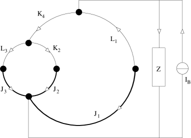
   Figure 1: The IBM qubit. This is an example of a network graph with 6 nodes and 15 branches. Each thick line represents a Josephson element, i.e. three branches in parallel, see Figure 2. Thin lines represent simple two-terminal elements, such as linear inductors (L, K), external impedances (Z), and current sources ($I_{B}$).

   

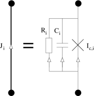
   Figure 2: A Josephson subgraph (thick line) consists of three branches; a Josephson junction (cross), a shunt capacitor (C), a shunt resistor (R), and no extra nodes.

   

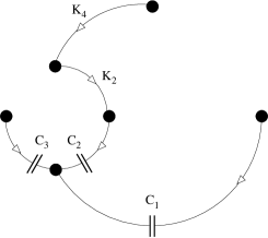
   Figure 3: A tree for the circuit shown in Figure 1. A tree is a subgraph containing all nodes and no loop. Here, we choose a tree that contains all capacitors (C), some inductors (K), but no current sources ($I_{B}$) or external impedances (Z).

3. Find the loop sub-matrices ${\bf F}_{CL}$, ${\bf F}_{CZ}$, ${\bf F}_{CB}$, ${\bf F}_{KL}$, ${\bf F}_{KZ}$, and ${\bf F}_{KB}$. The loop sub-matrices have entries $+1$, $-1$, or $0$, and hold the information about the important interconnections in the circuit. The matrix ${\bf F}_{XY}$ determines which tree branches $X$ (either capacitors, $X=C$, or inductors $X=K$) are present in which loop defined by the chords $Y$ (inductors, $Y=L$, external impedances $Y=Z$, or current sources, $Y=B$). In order to find, e.g., the loop sub-matrix ${\bf F}_{CL}$ for the IBM circuit (Figs. 1 and 3), we have to identify all loops obtained by adding a chord inductor ($L$). Each column in ${\bf F}_{CL}$ corresponds to one such loop. In our example, there are two chord inductors $L_{1}$ and $L_{3}$; the corresponding loops are the main superconducting loop (large circle) and the control loop (small circle). Each row in ${\bf F}_{CL}$ stands for one capacitor $C$; therefore, in our example, ${\bf F}_{CL}$ is a 3 by 2 matrix. The entries in each column of ${\bf F}_{CL}$ are $1$, $-1$, or $0$, depending on whether the corresponding capacitor (row) belongs to the corresponding loop (column) with the same ($-1$) or opposite ($+1$) orientation or does not belong to the loop at all ($0$). E.g., for our example, [cf. Eq. (172)]

   $${\bf F}_{CL}=\left(\begin{array}[]{r r}1&0\\ -1&1\\ 0&-1\end{array}\right).$$

   The first column says that the capacitor $C_{1}$ (part of $J_{1}$) belongs to the large loop (in the opposite direction, thus $+1$), capacitor $C_{2}$ (part of $J_{2}$) belongs to the large loop (in the same direction, thus $-1$), while capacitor $C_{3}$ (part of $J_{3}$) does not belong to the large loop at all. Similarly, the second column of ${\bf F}_{CL}$ says which of the capacitors are contained in the small loop.

4. Use the inductances (self and mutual)

   $${\bf L}_{\rm t}=\left(\begin{array}[]{c c}{\bf L}&{\bf L}_{LK}\\ {\bf L}_{LK}^{T}&{\bf L}_{K}\end{array}\right)$$ (1)

   and external impedances ${\bf Z}(\omega)$ to calculate the matrices ${\bf M}_{0}$, ${\bf N}$, $\bar{\bf m}$, ${\bf S}$ using Eqs. (77),(78), (80) and (81); for a single external impedance, also use Eqs. (88)–(90) to calculate the function $K(\omega)$, the coupling strength $\mu$ and the unit vector ${\bf m}$. The block form of the inductance matrix ${\bf L}_{\rm t}$ originates from the distinction between tree (K) and chord (L) inductors; ${\bf L}$ is the chord inductance matrix (including chord-chord mutual inductances as its off-diagonal elements), ${\bf L}_{K}$ is the tree inductance matrix, and ${\bf L}_{LK}$ is the tree-chord mutual inductance matrix. The Hamiltonian, Eqs. (92)–(97), together with the bath spectral density $J(\omega)\propto{\rm Im}K(\omega)$, Eq. (108), represents the quantum theory of the system including the dissipative environment. The form of this Hamiltonian, in particular the Equations (77)–(81) are the first main results of this paper. The evolution of the density matrix $\rho$ of the superconducting phases only is determined by the Bloch-Redfield equation (122) with the Redfield tensor given by Eqs. (LABEL:RGamma) and (V), representing our second main result.

5. Find the eigenstates and eigenenergies of the system Hamiltonian Eq. (93) and calculate the matrix elements of the superconducting phase operators $\varphi$. In practice, this task is usually done numerically or using some approximation. Typically, only a finite number of eigenstates is known.

6. For two given quantum levels $|0\rangle$ and $|1\rangle$, the relaxation time $T_{1}$ and pure dephasing time $T_{\phi}$ can be found using Eqs. (139) and (140); the decoherence time is then given by

   $$\frac{1}{T_{2}}=\frac{1}{2T_{1}}+\frac{1}{T_{\phi}}.$$

   The leakage rate $T_{L}^{-1}$ is given by Eq. (165).

We have carried out the above program for two cases; for the IBM qubit IBM (Fig. 1) in Sec. VIII and for the Delft qubit Mooij ; Orlando (Fig. 6) in Sec. IX. For the IBM qubit, matrix elements were calculated numerically; the relaxation and decoherence times in the case of a current-biased circuit are plotted in Fig. 4. For the Delft qubit, a semiclassical approach was taken, and earlier results by van der Wal et al. WWHM for a symmetric SQUID are correctly reproduced. In addition to this, the effect of SQUID asymmetries–either in the self inductance or in the critical currents of the two junctions–are calculated in Sec. IX.3. It turns out that typical sample-to-sample fluctuations of the critical current of about 10% can lead to a sizable decoherence rate at zero bias current.

III Classical network theory

The goal of this section is to derive a classical Hamiltonian for an electrical circuit containing superconducting elements, such as Josephson junctions. An electric circuit will be represented by an oriented graph Peikari ${\cal G}=({\cal N},{\cal B})$, see Fig. 1 for an example.

III.1 Graph theory

An oriented graph ${\cal G}=({\cal N},{\cal B})$ consists of $N$ nodes ${\cal N}=\{n_{1},\ldots,n_{N}\}$ and $B$ branches ${\cal B}=\{b_{1},\ldots,b_{B}\}$. In circuit analysis, a branch $b_{i}=(n_{a(i)},n_{b(i)})$ represents a two-terminal element (resistor, capacitor, inductor, current or voltage source, etc.), connecting its beginning node $n_{a(i)}$ to its ending node $n_{b(i)}$. The degree of a node $n\in{\cal N}$ is the number of branches containing $n$. A loop in ${\cal G}$ is a subgraph of ${\cal G}$ in which all nodes have degree 2. The number of disjoint connected subgraphs which, taken together, make up ${\cal G}$, will be denoted $P$ and the subgraphs ${\cal G}_{i}$, each having $N_{i}$ nodes and $B_{i}$ branches ($i=1,\ldots,P$), where $\sum_{i=1}^{P}N_{i}=N$ and $\sum_{i=1}^{P}B_{i}=B$. For each connected subgraph we choose a tree ${\cal T}_{i}$, i.e. a connected subgraph of ${\cal G}_{i}$ which contains all its nodes and has no loops. Note that ${\cal T}_{i}$ has exactly $N_{i}-1$ branches. The $B_{i}-N_{i}+1$ branches that do not belong to the tree are called chords. The tree of the graph ${\cal G}$ is the union of the trees of all its subgraphs, ${\cal T}_{i}$, containing $N-P$ branches. A tree of the graph shown in Fig. 1 is shown in Fig. 3. The fundamental loops ${\cal F}_{i}$ of a subgraph ${\cal G}_{i}$ are defined as the set of loops in ${\cal G}_{i}$ which contain exactly one chord $f_{i}\in{\cal G}_{i}\backslash{\cal T}_{i}$. We define the orientation of a fundamental loop via the orientation of its chord $f_{i}$. Each connected subgraph ${\cal G}_{i}$ has $F_{i}=B_{i}-N_{i}+1$ fundamental loops, i.e. the graph has $F=\sum_{i=1}^{P}F_{i}=B-N+P$ fundamental loops (one for each chord). A cutset of a connected graph is a set of a minimum number of branches that, when deleted, divides the graph into two separate subgraphs. A fundamental cutset of a graph with respect to a tree is a cutset that is made up of one tree branch $c_{i}$ and a unique set of chords. We denote the set of fundamental cutsets of ${\cal G}_{i}$ with respect to the tree ${\cal T}_{i}$ with ${\cal C}_{i}$. Each connected subgraph has $N_{i}-1$ fundamental cutsets, therefore there are $N-P$ fundamental cutsets in total (one for each tree branch).

We will use two characteristic matrices of the network graph, the fundamental loop matrix ($i=1,\ldots F$; $j=1,\ldots,B$),

$${\bf F}^{(L)}_{ij}=\left\{\begin{array}[]{l l}1,&\mbox{if $b_{j}\in{\cal F}_{i}$ (same direction as $f_{i}$)},\\ -1,&\mbox{if $b_{j}\in{\cal F}_{i}$ (direction opposite to $f_{i}$)},\\ 0,&\mbox{if $b_{j}\not\in{\cal F}_{i}$},\end{array}\right.$$ (2)

and the fundamental cutset matrix ($i=1,\ldots,N+P$; $j=1,\ldots,B$),

$${\bf F}^{(C)}_{ij}=\left\{\begin{array}[]{l l}1,&\mbox{if $b_{j}\in{\cal C}_{i}$ (same direction as $c_{i}$)},\\ -1,&\mbox{if $b_{j}\in{\cal C}_{i}$ (direction opposite to $c_{i}$)},\\ 0,&\mbox{if $b_{j}\not\in{\cal C}_{i}$}.\end{array}\right.$$ (3)

By observing that cutsets always intersect loops in as many ingoing as outgoing branches, one finds

$${\bf F}^{(L)}\left({\bf F}^{(C)}\right)^{T}=0,$$ (4)

By labeling the branches of the graph ${\cal G}$ such that the first $N-P$ branches belong to the tree ${\cal T}$, we obtain

$${\bf F}^{(C)}=\left(\openone\,|\,{\bf F}\right),$$ (5)

where ${\bf F}$ is an $(N+P)\times(B-N-P)$ matrix. Using Eq. (4), we find

$${\bf F}^{(L)}=\left(-{\bf F}^{T}\,|\,\openone\right).$$ (6)

III.2 Electric circuits

The state of an electric circuit described by a network graph can be defined by the branch currents ${\bf I}=(I_{1},\ldots I_{B})$, where $I_{i}$ denotes the electric current flowing in branch $b_{i}$, and the branch voltages ${\bf V}=(V_{1},\ldots V_{B})$, where $V_{i}$ denotes the voltage drop across the branch $b_{i}$. The sign of $I_{i}$ is positive if a positive current flows from node $n_{a(i)}$ to $n_{b(i)}$ and negative if a positive current flows from node $n_{b(i)}$ to $n_{a(i)}$; $V_{i}$ is positive if the electric potential is higher at node $n_{a(i)}$ than at node $n_{b(i)}$.

The conservation of electrical current, combined with the condition that no charge can be accumulated at a node, implies Kirchhoff’s current law,

$${\bf F}^{(C)}{\bf I}=0.$$ (7)

In a lumped circuit, energy conservation implies Kirchhoff’s voltage law in the form

$${\bf F}^{(L)}{\bf V}=0.$$ (8)

External magnetic fluxes ${\bf\Phi}=(\Phi_{1},\ldots,\Phi_{B-N+P})$ threading the loops of the circuit represent a departure from the strict lumped circuit model; if they are present, Faraday’s law requires that

$${\bf F}^{(L)}{\bf V}={\bf\dot{\Phi}}.$$ (9)

External fluxes have to be distinguished from the fluxes associated with lumped circuit elements (e.g., inductors, see below).

We divide the branch currents and voltages into a tree and a chord part,

$${\bf I} = ({\bf I}_{\rm tr},{\bf I}_{\rm ch}),$$ (10)

$${\bf V} = ({\bf V}_{\rm tr},{\bf V}_{\rm ch}).$$ (11)

The $2B$ branch currents and voltages are not independent; the Kirchhoff laws Eqs. (7) and (9) together with Eqs. (5) and (6) yield the following $B$ equations relating them,

$${\bf F}{\bf I}_{\rm ch} = -{\bf I}_{\rm tr},$$ (12)

$${\bf F}^{T}{\bf V}_{\rm tr} = {\bf V}_{\rm ch}-{\bf\dot{\Phi}}.$$ (13)

As an example, the $N+P$ tree branch voltages ${\bf V}_{\rm tr}$ combined with the $B-N-P$ chord currents ${\bf I}_{\rm ch}$ completely describe the state of a network, since all other currents and voltages can be obtained from them via Eqs. (12) and (13). However, in the following, we will use a different subset of variables, also making use of the $B$ equations that are derived from the current-voltage relations of the individual branch elements.

III.3 Circuits containing superconducting elements

For the purpose of analyzing electric circuits containing Josephson junctions, we adopt the RSJ model for a Josephson junction, i.e. a junction shunted by a capacitor and a resistor, see Fig. 3. We treat the Josephson junctions as nonlinear inductors. A (flux controlled) nonlinear inductor Peikari is a two-terminal circuit element that follows a relation between the time-dependent current $I(t)$ flowing through it and the voltage $V(t)$ across it of the form

$$I(t)=f(\Phi(t)),$$ (14)

where $\dot{\Phi}(t)\equiv V(t)$ and $f$ is an arbitrary function. For a linear inductor, $f(x)=x/L$, with $L$ the inductance.

We begin our analysis by choosing a tree containing all of the capacitors in the network, no resistors or external impedances, no current sources, and as few inductors as possible (in particular, no Josephson junctions). We assume here that the network does not contain any capacitor-only loops, which is realistic because in practice any loop has a nonzero inductance. A network is called proper if in addition to this, it is possible to choose a tree without any inductors (i.e., if there are no inductor-only cutsets) Peikari . Again, it can be argued that this is realistic since there always are (at least small) capacitances between different parts of a network. But we have avoided making the latter assumption here because it spares us from describing the dynamics of small parasitic capacitances. We further assume that each Josephson junction is shunted by a finite capacitance, so that we are able to choose a tree without any Josephson junctions. Finally, we assume for simplicity that the circuit does not contain any voltage sources; however, voltage sources could easily be incorporated into our analysis.

We divide up the tree and chord currents and voltages further, according to the various branch types,

$${\bf I}_{\rm tr}=({\bf I}_{C},{\bf I}_{K}), {\bf I}_{\rm ch}=({\bf I}_{J},{\bf I}_{L},{\bf I}_{R},{\bf I}_{Z},{\bf I}_{B}),$$ (15)

$${\bf V}_{\rm tr}=({\bf V}_{C},{\bf V}_{K}), {\bf V}_{\rm ch}=({\bf V}_{J},{\bf V}_{L},{\bf V}_{R},{\bf V}_{Z},{\bf V}_{B}),\quad\quad$$ (16)

where the tree current and voltage vectors contain a capacitor (C) and tree inductor (K) part, whereas the chord current and voltage vectors consist of parts for chord inductors, both non-linear (J) and linear (L), shunt resistors (R) and other external impedances (Z), and bias current sources (B). Accordingly, we write

$${\bf F}=\left(\begin{array}[]{c c c c c}{\bf F}_{CJ}&{\bf F}_{CL}&{\bf F}_{CR}&{\bf F}_{CZ}&{\bf F}_{CB}\\ {\bf F}_{KJ}&{\bf F}_{KL}&{\bf F}_{KR}&{\bf F}_{KZ}&{\bf F}_{KB}\end{array}\right).$$ (19)

The sub-matrices ${\bf F}_{XY}$ will be called loop sub-matrices. Note that since Josephson junctions are always shunted by a capacitor as a tree branch, there are never any tree inductors in parallel with a Josephson junction, ${\bf F}_{KJ}={\bf 0}$. As a consequence, a tree inductor is never in parallel with a shunt resistor, ${\bf F}_{KR}={\bf 0}$.

We then formally define the branch charges and fluxes ($X=C,K,J,L,R,Z,B$),

$${\bf I}_{X}(t) = \dot{\bf Q}_{X}(t),$$ (20)

$${\bf V}_{X}(t) = \dot{\bf\Phi}_{X}(t).$$ (21)

Using the second Josephson relation and Eq. (21), we identify the formal fluxes associated with the Josephson junctions as the superconducting phase differences $\varphi$ across the junctions,

$$\frac{{\bf\Phi}_{J}}{\Phi_{0}}=\frac{{\mbox{\boldmath$\varphi$}}}{2\pi},$$ (22)

where $\Phi_{0}=h/2e$ is the superconducting flux quantum. It will be assumed that at some initial time $t_{0}$ (which can be taken as $t_{0}\rightarrow-\infty$), all charges and fluxes (including the external fluxes) are zero, ${\bf Q}_{X}=0$, ${\bf\Phi}_{X}=0$ (including ${\mbox{\boldmath$\varphi$}}=0$), and ${\bf\Phi}=0$.

The current-voltage relations for the various types of branches are

$${\bf I}_{J} = {\bf I}_{\rm c}\,\mbox{\boldmath$\sin$}{\mbox{\boldmath$\varphi$}},$$ (23)

$${\bf Q}_{C} = {\bf C}{\bf V}_{C},$$ (24)

$${\bf I}_{L} = \bar{\bf L}^{-1}{\bf\Phi}_{L}-{\bf L}^{-1}{\bf L}_{LK}\bar{\bf L}_{K}^{-1}{\bf\Phi}_{K},$$ (25)

$${\bf I}_{K} = \bar{\bf L}_{K}^{-1}{\bf\Phi}_{K}-{\bf L}_{K}^{-1}{\bf L}_{LK}^{T}\bar{\bf L}^{-1}{\bf\Phi}_{L},$$ (26)

$${\bf V}_{R} = {\bf R}{\bf I}_{R},$$ (27)

$${\bf V}_{Z}(\omega) = {\bf Z}(\omega){\bf I}_{Z}(\omega),$$ (28)

where Eq. (23) is the first Josephson relation for the Josephson junctions (flux-controlled non-linear inductors), where the diagonal matrix ${\bf I}_{\rm c}$ contains the critical currents $I_{{\rm c},i}$ of the junctions on its diagonal, and $\mbox{\boldmath$\sin$}{\mbox{\boldmath$\varphi$}}\equiv(\sin\varphi_{1},\sin\varphi_{2},\ldots,\sin\varphi_{N_{J}})$. Eq. (24) describes the (linear) capacitors (${\bf C}$ is the capacitance matrix), Eqs. (25) and (26) the linear inductors, see Eqs. (43) and (44) below. The junction shunt resistors are described by Eq. (27) where $R$ is the (diagonal and real) shunt resistance matrix. The external impedances are described by the relation Eq. (28) between the Fourier transforms of the current and voltage, where ${\bf Z}(\omega)$ is the impedance matrix. The external impedances can also defined in the time domain,

$${\bf V}_{Z}(t)=\int_{-\infty}^{t}{\bf Z}(t-\tau){\bf I}_{Z}(\tau)d\tau\equiv({\bf Z}*{\bf I}_{Z})(t),$$ (29)

where the convolution is defined as

$$({\bf f}*{\bf g})(t)=\int_{-\infty}^{t}{\bf f}(t-\tau){\bf g}(\tau)d\tau.$$ (30)

Causality allows the response function to be nonzero only for positive times, ${\bf Z}(t)=0$ for $t<0$. In frequency space, the replacement $\omega\rightarrow\omega+i\epsilon$ with $\epsilon>0$ guarantees convergence of the Fourier transform

$${\bf Z}(\omega)=\int_{-\infty}^{\infty}{\bf Z}(t)e^{i\omega t}dt=\int_{0}^{\infty}{\bf Z}(t)e^{i\omega t}dt.$$ (31)

In order to obtain Eq. (25) for the inductors, we write

$$\left(\begin{array}[]{c}{\bf\Phi}_{L}\\ {\bf\Phi}_{K}\end{array}\right)=\left(\begin{array}[]{l l}{\bf L}&{\bf L}_{LK}\\ {\bf L}_{LK}^{T}&{\bf L}_{K}\end{array}\right)\left(\begin{array}[]{c}{\bf I}_{L}\\ {\bf I}_{K}\end{array}\right)\equiv{\bf L}_{\rm t}\left(\begin{array}[]{c}{\bf I}_{L}\\ {\bf I}_{K}\end{array}\right),$$ (32)

where ${\bf L}$ and ${\bf L}_{K}$ are the self inductances of the chord and tree branch inductors, resp., off-diagonal elements describing the mutual inductances among chord inductors and tree inductors separately, and ${\bf L}_{LK}$ is the mutual inductance matrix between tree and chord inductors. Since the total inductance matrix is symmetric and positive, i.e. ${\bf v}^{T}{\bf L}_{\rm t}{\bf v}>0$ for all real vectors ${\bf v}$, its inverse exists, and we find

$$\left(\begin{array}[]{c}{\bf I}_{L}\\ {\bf I}_{K}\end{array}\right) = \left(\begin{array}[]{c c}\bar{\bf L}^{-1}&-{\bf L}^{-1}{\bf L}_{LK}\bar{\bf L}_{K}^{-1}\\ -{\bf L}_{K}^{-1}{\bf L}_{LK}^{T}\bar{\bf L}^{-1}&\bar{\bf L}_{K}^{-1}\end{array}\right)\left(\begin{array}[]{c}{\bf\Phi}_{L}\\ {\bf\Phi}_{K}\end{array}\right)$$ (39)

$$\equiv {\bf L}_{\rm t}^{-1}\left(\begin{array}[]{c}{\bf\Phi}_{L}\\ {\bf\Phi}_{K}\end{array}\right)$$ (42)

with the definitions

$$\bar{\bf L} = {\bf L}-{\bf L}_{LK}{\bf L}_{K}^{-1}{\bf L}_{LK}^{T},$$ (43)

$$\bar{\bf L}_{K} = {\bf L}_{K}-{\bf L}_{LK}^{T}{\bf L}^{-1}{\bf L}_{LK}.$$ (44)

Note that the matrices ${\bf L}$ and ${\bf L}_{K}$, being diagonal sub-matrices of a symmetric and positive matrix, are also symmetric and positive and thus their inverses exist. The operators $\bar{\bf L}$ and $\bar{\bf L}_{K}$ as defined in Eqs. (43) and (44) are invertible since ${\bf L}_{\rm t}^{-1}$ exists. Moreover, since the inverse of the total inductance matrix, see Eq. (42), is symmetric and positive, its diagonal sub-matrices are symmetric and positive, and thus $\bar{\bf L},\bar{\bf L}_{K}>0$.

III.4 Equations of motion

In order to derive a Lagrangian for an electric circuit, we have to single out among the charges and fluxes a complete set of unconstrained degrees of freedom, such that each assignment of values to those charges and fluxes and their first time derivatives represents a possible dynamical state of the system. Using Eqs. (19–21), (23–28), (32), and (42), the time evolution of the charges and fluxes can be expressed as the following set of first-order integro-differential equations

$$\frac{\Phi_{0}}{2\pi}\dot{\mbox{\boldmath$\varphi$}} = {\bf V}_{J}={\bf F}_{CJ}^{T}{\bf C}^{-1}{\bf Q}_{C},$$ (45)

$$\dot{\bf Q}_{C} = {\bf I}_{C}=-{\bf F}_{CJ}{\bf I}_{\rm c}\,\mbox{\boldmath$\sin$}{\mbox{\boldmath$\varphi$}}-{\bf F}_{CR}{\bf R}^{-1}\dot{\bf\Phi}_{R}$$ (46)

$$-{\bf F}_{CL}\left(\bar{\bf L}^{-1}{\bf\Phi}_{L}-{\bf L}^{-1}{\bf L}_{LK}\bar{\bf L}_{K}^{-1}{\bf\Phi}_{K}\right)$$

$$-{\bf F}_{CZ}{\bf L}_{Z}^{-1}*{\bf\Phi}_{Z}-{\bf F}_{CB}{\bf I}_{B},$$

$$\dot{\bf\Phi}_{L} = {\bf V}_{\rm L}={\bf F}_{CL}^{T}{\bf C}^{-1}{\bf Q}_{C}+{\bf F}_{KL}^{T}\dot{\bf\Phi}_{K}+\dot{\bf\Phi}_{x},$$ (47)

$$\dot{\bf\Phi}_{R} = {\bf V}_{\rm R}={\bf F}_{CR}^{T}{\bf C}^{-1}{\bf Q}_{C},$$ (48)

$$\dot{\bf\Phi}_{Z} = {\bf V}_{\rm Z}={\bf F}_{CZ}^{T}{\bf C}^{-1}{\bf Q}_{C}+{\bf F}_{KZ}^{T}\dot{\bf\Phi}_{K},$$ (49)

$${\bf\Phi}_{K} = -{\bf L}_{K}\bar{\bf F}_{KL}\bar{\bf L}^{-1}{\bf\Phi}_{L}+{\bf L}_{K}\bar{\bf F}_{KL}{\bf L}^{-1}{\bf L}_{LK}\bar{\bf L}_{K}^{-1}{\bf\Phi}_{K}$$ (50)

$$-{\bf L}_{K}{\bf F}_{KZ}{\bf L}_{Z}^{-1}*{\bf\Phi}_{Z}-{\bf L}_{K}{\bf F}_{KB}{\bf I}_{B},\quad$$

where ${\bf L}_{Z}(\omega)\equiv{\bf Z(\omega)}/i\omega$, and where the convolution is given by Eq. (30). In the equations for the chord variables Eqs. (45), (47), (48), and (49), we have assumed that only the loops closed by a chord inductor (L) are threaded by an external flux, ${\bf\Phi}=(0,{\bf\Phi}_{x},0,0,0)$. In order to obtain Eq. (50), we have first used Eq. (32), then Eqs. (12) and (28), and finally Eq. (42). We can eliminate ${\bf\Phi}_{K}$ by solving Eq. (50),

$${\bf\Phi}_{K}=-\tilde{\bf L}_{K}\left(\bar{\bf F}_{KL}\bar{\bf L}^{-1}{\bf\Phi}_{L}+{\bf F}_{KZ}{\bf L}_{Z}^{-1}*{\bf\Phi}_{Z}+{\bf F}_{KB}{\bf I}_{B}\right),$$ (51)

with the definitions

$$\tilde{\bf L}_{K} = \left(\openone_{K}-{\bf L}_{K}\bar{\bf F}_{KL}{\bf L}^{-1}{\bf L}_{LK}\bar{\bf L}_{K}^{-1}\right)^{-1}{\bf L}_{K},$$ (52)

$$\bar{\bf F}_{KL} = {\bf F}_{KL}-{\bf L}_{K}^{-1}{\bf L}_{LK}^{T}.$$ (53)

Further knowledge of the structure of ${\bf F}$ can be derived from the fact that Josephson junctions are always assumed to be RC-shunted, see Fig. 2. If we label the tree branches such that the first $N_{J}\leq N_{C}$ capacitances are the ones shunting the Josephson junctions ($N_{C}$=number of capacitances, $N_{J}$=number of Josephson junctions) then we find

$${\bf F}_{CJ} = {\bf F}_{CR}=\left(\begin{array}[]{c}\openone_{N_{J}}\\ 0_{N_{C}-N_{J}}\end{array}\right),$$ (56)

$${\bf Q}_{C} = \left(\begin{array}[]{c}{\bf Q}_{CJ}\\ {\bf Q}_{\bar{C}}\end{array}\right),$$ (59)

where $\bar{C}$ denotes the capacitors which are not parallel shunts of a Josephson junction. In general, the charges of these additional capacitors represent independent degrees of freedom in addition to the shunt capacitor charges ${\bf Q}_{CJ}=\Phi_{0}{\bf C}\dot{\mbox{\boldmath$\varphi$}}/2\pi$. But from this point onward, we will study the case where there are no capacitors except the Josephson junction shunt capacitors, $N_{C}=N_{J}$. However, the resulting equation of motion (76) with the definitions Eqs. (77)–(81) still allows us to describe pure capacitors by treating them as Josephson elements with zero critical current $I_{c}$ and infinite shunt resistance $R$. With this simplification,

$${\bf F}_{CJ}={\bf F}_{CR}=\openone,$$ (60)

and the $\varphi$ and $\dot{\mbox{\boldmath$\varphi$}}$ can be chosen as the $2N_{J}$ generalized coordinates and velocities that satisfy the equation of motion

$${\bf C}\ddot{\mbox{\boldmath$\varphi$}} = -{\bf L}_{J}^{-1}\mbox{\boldmath$\sin$}{\mbox{\boldmath$\varphi$}}-{\bf R}^{-1}\dot{\mbox{\boldmath$\varphi$}}$$

$$-\frac{2\pi}{\Phi_{0}}\left({\bf F}_{CL}\tilde{\bf L}_{L}^{-1}{\bf\Phi}_{L}+\bar{\bf F}_{CZ}{\bf L}_{Z}^{-1}*{\bf\Phi}_{Z}+\bar{\bf F}_{CB}{\bf I}_{B}\right),$$

where we have used Eqs. (45), (46), and (51), and introduced ${\bf L}_{J}^{-1}=2\pi{\bf I}_{\rm c}/\Phi_{0}$, and ($Y=Z,B$)

$$\tilde{\bf L}_{L}^{-1} = \left(\openone_{L}+{\bf L}^{-1}{\bf L}_{LK}\bar{\bf L}_{K}^{-1}\tilde{\bf L}_{K}\bar{\bf F}_{KL}\right)\bar{\bf L}^{-1},$$ (62)

$$\bar{\bf F}_{CY} = {\bf F}_{CY}+{\bf F}_{CL}{\bf L}^{-1}{\bf L}_{LK}\bar{\bf L}^{-1}_{K}\tilde{\bf L}_{K}{\bf F}_{KY}.$$ (63)

The remaining state variables obey the following linear relations,

$${\bf L}_{LL}\bar{\bf L}^{-1}\dot{\bf\Phi}_{L}+{\bf L}_{LZ}{\bf L}_{Z}^{-1}*\dot{\bf\Phi}_{Z} = {\bf a}_{L}(\dot{\mbox{\boldmath$\varphi$}}),$$ (64)

$${\bf L}_{ZL}\bar{\bf L}^{-1}\dot{\bf\Phi}_{L}+{\bf L}_{ZZ}{\bf L}_{Z}^{-1}*\dot{\bf\Phi}_{Z} = {\bf a}_{Z}(\dot{\mbox{\boldmath$\varphi$}}),$$ (65)

where we have introduced

$${\bf L}_{LL} = \bar{\bf L}+{\bf F}_{KL}^{T}\tilde{\bf L}_{K}\bar{\bf F}_{KL},$$ (66)

$${\bf L}_{ZZ} = {\bf L}_{Z}+{\bf F}_{KZ}^{T}\tilde{\bf L}_{K}{\bf F}_{KZ},$$ (67)

$${\bf L}_{LZ} = {\bf F}_{KL}^{T}\tilde{\bf L}_{K}{\bf F}_{KZ},$$ (68)

$${\bf L}_{ZL} = {\bf F}_{KZ}^{T}\tilde{\bf L}_{K}\bar{\bf F}_{KL},$$ (69)

$${\bf a}_{L}(\dot{\mbox{\boldmath$\varphi$}}) = \frac{\Phi_{0}}{2\pi}{\bf F}_{CL}^{T}\dot{\mbox{\boldmath$\varphi$}}+\dot{\bf\Phi}_{x}-{\bf F}_{KL}^{T}\tilde{\bf L}_{K}{\bf F}_{KB}\dot{\bf I}_{B},$$ (70)

$${\bf a}_{Z}(\dot{\mbox{\boldmath$\varphi$}}) = \frac{\Phi_{0}}{2\pi}{\bf F}_{CZ}^{T}\dot{\mbox{\boldmath$\varphi$}}-{\bf F}_{KZ}^{T}\tilde{\bf L}_{K}{\bf F}_{KB}\dot{\bf I}_{B}.$$ (71)

Note that in the absence of dissipation, ${\bf L}_{Z}^{-1}\rightarrow{\bf 0}$, Eqs. (64) and (65) are holonomic constraints for the variables $\dot{\bf\Phi}_{L}$, since Eqs. (64) and (65) can be integrated. If ${\bf L}_{LL}$, ${\bf L}_{ZZ}$, and

$$\bar{\bf L}_{L} = {\bf L}_{LL}-{\bf L}_{LZ}{\bf L}_{ZZ}^{-1}{\bf L}_{ZL},$$ (72)

$$\bar{\bf L}_{Z} = {\bf L}_{ZZ}-{\bf L}_{ZL}{\bf L}_{LL}^{-1}{\bf L}_{LZ},$$ (73)

are regular matrices, the solution to Eqs. (64) and (65) is given by

$$\dot{\bf\Phi}_{L} = \bar{\bf L}\bar{\bf L}_{L}^{-1}\left({\bf a}_{L}(\dot{\mbox{\boldmath$\varphi$}})-{\bf L}_{LZ}{\bf L}_{ZZ}^{-1}*{\bf a}_{Z}(\dot{\mbox{\boldmath$\varphi$}})\right),$$ (74)

$$\dot{\bf\Phi}_{Z} = {\bf L}_{Z}\bar{\bf L}_{Z}^{-1}*\left({\bf a}_{Z}(\dot{\mbox{\boldmath$\varphi$}})-{\bf L}_{ZL}{\bf L}_{LL}^{-1}{\bf a}_{L}(\dot{\mbox{\boldmath$\varphi$}})\right).$$ (75)

Note that in the limit of large external impedances, ${\bf L}_{Z}\rightarrow{\bf 0}$, the regularity conditions for ${\bf L}_{LL}$, ${\bf L}_{ZZ}$, $\bar{\bf L}_{L}$, and $\bar{\bf L}_{Z}$ all collapse to the condition that ${\bf L}_{LL}$ be regular. The latter always holds in the absence of mutual inductances between tree and chord inductors, since in this case $\bar{\bf F}_{KL}={\bf F}_{KL}$ and thus ${\bf L}_{LL}$ is symmetric and positive, so that its inverse exists. Integrating Eqs. (74) and (75) from $t_{0}$ to $t$, using the initial condition (all charges and fluxes equal to zero), and substituting the solutions into Eq. (III.4), we arrive at the classical equation of motion for the superconducting phases $\varphi$,

$${\bf C}\ddot{\mbox{\boldmath$\varphi$}}=-{\bf L}_{J}^{-1}{\mbox{\boldmath$\sin$}}{\mbox{\boldmath$\varphi$}}-{\bf R}^{-1}\dot{\mbox{\boldmath$\varphi$}}-{\bf M}_{0}{\mbox{\boldmath$\varphi$}}-{\bf M}_{d}*{\mbox{\boldmath$\varphi$}}-\frac{2\pi}{\Phi_{0}}{\bf N}{\bf\Phi}_{x}-\frac{2\pi}{\Phi_{0}}{\bf S}{\bf I}_{B},$$ (76)

with

$${\bf M}_{0} = {\bf F}_{CL}\tilde{\bf L}_{L}^{-1}\bar{\bf L}{\bf L}_{LL}^{-1}{\bf F}_{CL}^{T},$$ (77)

$${\bf N} = {\bf F}_{CL}\tilde{\bf L}_{L}^{-1}\bar{\bf L}{\bf L}_{LL}^{-1},$$ (78)

$${\bf M}_{d}(\omega) = \bar{\bf m}\bar{\bf L}_{Z}^{-1}(\omega)\bar{\bf m}^{T},$$ (79)

$$\bar{\bf m} = {\bf F}_{CZ}-{\bf F}_{CL}({\bf L}_{LL}^{-1})^{T}\bar{\bf F}_{KL}^{T}\tilde{\bf L}_{K}^{T}{\bf F}_{KZ},$$ (80)

$${\bf S} = {\bf F}_{CB}-{\bf F}_{CL}({\bf L}_{LL}^{-1})^{T}\bar{\bf F}_{KL}^{T}\tilde{\bf L}_{K}^{T}{\bf F}_{KB}.$$ (81)

Although the expression (77) for the matrix ${\bf M}_{0}$ is not manifestly symmetric, we show in Appendix A that it is indeed symmetric, i.e. ${\bf M}_{0}^{T}={\bf M}_{0}$. This property of ${\bf M}_{0}$ allows us to write the term ${\bf M}_{0}{\mbox{\boldmath$\varphi$}}$ in the equations of motion (76) as the gradient of a potential, see Eq. (92) below. The matrices ${\bf M}_{d}(\omega)$ and ${\bf R}$ contain all the dissipative dynamics of $\varphi$; if all external impedances (shunt resistors) are removed, then ${\bf L}_{Z}^{-1}\rightarrow{\bf 0}$ and thus ${\bf M}_{d}(\omega)\rightarrow{\bf 0}$ (${\bf R}^{-1}\rightarrow 0$). A proof of the symmetry of the dissipation matrix, ${\bf M}_{d}={\bf M}_{d}^{T}$, and a derivation of the representation in Eqs. (79) and (80) can be found in Appendix B.

Note that the coupling matrix ${\bf S}$ to an external bias current ${\bf I}_{B}$ can be obtained from $\bar{\bf m}$ by replacing $Z$ by $B$. Physically, this means that the external impedances $Z$ can be thought of as fluctuating external currents; in particular, if a bias current is shunted in parallel to an impedance, ${\bf F}_{XZ}=\pm{\bf F}_{XB}$ ($X=C,K$) then we find ${\bf S}=\pm\bar{\bf m}$. In deriving the equation of motion (76), we have assumed that the external magnetic fluxes and bias currents become time-independent after they have been switched on in the past, $\dot{\bf\Phi}_{x}\rightarrow 0$, $\dot{\bf I}_{B}\rightarrow 0$ ($t>t_{0}$). In the absence of mutual inductances between the tree and chord inductors, ${\bf L}_{KL}={\bf 0}$, Eqs. (77)–(81) become somewhat simpler,

$${\bf M}_{0} = {\bf F}_{CL}{\bf L}_{LL}^{-1}{\bf F}_{CL}^{T},$$ (82)

$${\bf N} = {\bf F}_{CL}{\bf L}_{LL}^{-1},$$ (83)

$$\bar{\bf m} = {\bf F}_{CZ}-{\bf F}_{CL}{\bf L}_{LL}^{-1}{\bf F}_{KL}^{T}{\bf L}_{K}{\bf F}_{KZ},$$ (84)

$${\bf S} = {\bf F}_{CB}-{\bf F}_{CL}{\bf L}_{LL}^{-1}{\bf F}_{KL}^{T}{\bf L}_{K}{\bf F}_{KB},$$ (85)

$${\bf L}_{LL} = {\bf L}+{\bf F}_{KL}^{T}{\bf L}_{K}{\bf F}_{KL}={\bf L}_{LL}^{T}.$$ (86)

It should be noted here that from now on, the shunt resistors ${\bf R}$ can be treated as external impedances by setting ${\bf M}_{d}^{\prime}={\bf M}_{d}+i\omega{\bf R}^{-1}$; the only reason for treating the shunt resistors separately is that more is known about the possible arrangement of the shunt resistors in the circuit. We will mostly concentrate on external impedances in our examples and neglect the shunt resistors, because in our examples $R\gg Z$. If, in turn, the external impedances are pure resistors, i.e. ${\bf Z}(\omega)$ is real and frequency independent, then they can be described as corrections to ${\bf R}$, i.e. ${\bf R}^{\prime}={\bf R}+{\bf Z}$.

A few important remarks about the form of the matrix ${\bf M}_{d}$ are in order. (i) We know that ${\bf M}_{d}(t)$ is real, causal (i.e., ${\bf M}_{d}(t)=0$ for $t<0$), and symmetric ${\bf M}_{d}={\bf M}_{d}^{T}$ (Appendix B). A dissipative term in the equations of motion with these properties can be modeled using the Caldeira-Leggett formalism CaldeiraLeggett . (ii) In the lowest-order Born approximation, i.e. perturbation theory in the equation of motion in the small parameters $Z_{i}^{-1}$ (see below), the contributions to ${\bf M}_{d}$ from different external impedances are additive, in the sense that one can calculate ${\bf M}_{d}$ for each impedance $Z_{i}$ separately, while $Z_{j\neq i}\rightarrow\infty$, and then add the contributions in order to obtain the full coupling Hamiltonian (see Eq. (97) below). In the same manner, the decoherence rates due to different impedances will be additive in the lowest-order Born approximation. An exact statement (independent of the Born approximation) can be made if $\bar{\bf L}_{Z}^{-1}$ can be written as a sum in which every term contains only one of the impedances $Z_{i}$, since in this case ${\bf M}_{d}=\sum_{i=1}^{N_{Z}}{\bf M}_{d,i}$ where $N_{Z}$ denotes the number of external impedances and ${\bf M}_{d,i}(\omega)$ describes the effect of $Z_{i}$. From now on, we will study the case of a single external impedance, bearing in mind that in lowest-order perturbation theory the results obtained in this way can easily be used to describe the dynamics of a system coupled to several external impedances. (iii) In the case of a single impedance, ${\bf M}_{d}(\omega)$ has the form,

$${\bf M}_{d}(\omega) = \mu K(\omega){\bf m}{\bf m}^{T},$$ (87)

$$K(\omega) = \bar{\bf L}_{Z}^{-1}(\omega),$$ (88)

$$\mu = |\bar{\bf m}|^{2},$$ (89)

$${\bf m} = \bar{\bf m}/\sqrt{\mu}=\bar{\bf m}/|\bar{\bf m}|,$$ (90)

where $K(t)$ is a scalar real function, ${\bf m}$ is the normalized vector parallel to $\bar{\bf m}$, and $\sqrt{\mu}$ is the length of the vector $\bar{\bf m}$ ($\mu$ is the eigenvalue of the rank 1 matrix $\bar{\bf m}\bar{\bf m}^{T}$).

The dissipation free (${\bf R},{\bf Z}\rightarrow\infty$, ${\bf M}_{d}=0$) part of the classical equation of motion Eq. (76) can be derived from the Lagrangian

$${\cal L}_{0} = \left(\frac{\Phi_{0}}{2\pi}\right)^{2}\left(\frac{1}{2}\dot{{\mbox{\boldmath$\varphi$}}}^{T}{\bf C}\dot{{\mbox{\boldmath$\varphi$}}}-U({\mbox{\boldmath$\varphi$}})\right),$$ (91)

$$U({\mbox{\boldmath$\varphi$}}) = -\sum_{i}L_{J;i}^{-1}\cos\varphi_{i}$$ (92)

$$+\frac{1}{2}{\mbox{\boldmath$\varphi$}}^{T}{\bf M}_{0}{\mbox{\boldmath$\varphi$}}+\frac{2\pi}{\Phi_{0}}{\mbox{\boldmath$\varphi$}}^{T}\left({\bf N}{\bf\Phi}_{x}+{\bf S}{\bf I}_{B}\right),$$

or, equivalently, from the Hamiltonian

$${\cal H}_{S}=\frac{1}{2}{\bf Q}_{C}^{T}{\bf C}^{-1}{\bf Q}_{C}+\left(\frac{\Phi_{0}}{2\pi}\right)^{2}U({\mbox{\boldmath$\varphi$}}),$$ (93)

where the canonical momenta corresponding to the flux variables $\Phi_{0}{\mbox{\boldmath$\varphi$}}/2\pi$ are the capacitor charges

$$\frac{2\pi}{\Phi_{0}}\frac{\partial{\cal L}_{0}}{\partial\dot{\mbox{\boldmath$\varphi$}}}=\frac{\Phi_{0}}{2\pi}{\bf C}\dot{\mbox{\boldmath$\varphi$}}={\bf C}{\bf V}_{C}\equiv{\bf Q}_{C}.$$

IV Canonical quantization of ${\cal H}_{S}$ and system-bath model

In this Section, we quantize the classical theory for a superconducting circuit that was derived in the previous Section. The conjugate flux and charge variables $\varphi$ and ${\bf Q}_{C}$ now have to be understood as operators with the commutation relations

$$\left[\frac{\Phi_{0}}{2\pi}\varphi_{i},Q_{C;j}\right]=i\hbar\delta_{ij}.$$ (94)

In order to include the dissipative dynamics of the classical equation of motion, Eq. (76), in our quantum description, we follow Caldeira and Leggett CaldeiraLeggett , and introduce a bath (reservoir) of harmonic oscillators describing the degrees of freedom of the external impedances. We will restrict ourselves to the case of a single external impedance coupled to the circuit (this is sufficient to describe the general case in the lowest-order Born approximation, see Sec. III). For the Hamiltonian of the circuit including the external impedance, we write

$${\cal H} = {\cal H}_{S}+{\cal H}_{B}+{\cal H}_{SB},$$ (95)

$${\cal H}_{B} = \frac{1}{2}\sum_{\alpha}\left(\frac{p_{\alpha}^{2}}{m_{\alpha}}+m_{\alpha}\omega_{\alpha}^{2}x_{\alpha}^{2}\right),$$ (96)

$${\cal H}_{SB} = {\bf m}\cdot{\mbox{\boldmath$\varphi$}}\sum_{\alpha}c_{\alpha}x_{\alpha}+\Delta U({\mbox{\boldmath$\varphi$}}),$$ (97)

where ${\cal H}_{S}$ is the quantized Hamiltonian Eq. (93), derived in Sec. III, ${\cal H}_{B}$ is the Hamiltonian describing a bath of harmonic oscillators with (fictitious) position and momentum operators $x_{\alpha}$ and $p_{\alpha}$ with $[x_{\alpha},p_{\beta}]=i\hbar\delta_{\alpha\beta}$, masses $m_{\alpha}$, and oscillator frequencies $\omega_{\alpha}$. Finally, ${\cal H}_{SB}$ describes the coupling between the system and bath degrees of freedom, $\varphi$ and $x_{\alpha}$, where $c_{\alpha}$ is a coupling parameter and ${\bf m}$ is defined in Eqs. (80) and (90). The term $\Delta U({\mbox{\boldmath$\varphi$}})=({\bf m}\cdot{\mbox{\boldmath$\varphi$}})^{2}\sum_{\alpha}c_{\alpha}^{2}/2m_{\alpha}\omega_{\alpha}^{2}$ compensates the energy renormalization caused by the system-bath interaction (first term) CaldeiraLeggett . It ensures that, for a fixed value of $\varphi$,

$$\min_{\{x_{\alpha}\}}\left[U({\mbox{\boldmath$\varphi$}})+{\cal H}_{B}(\{x_{\alpha}\})+{\cal H}_{SB}({\mbox{\boldmath$\varphi$}},\{x_{\alpha}\})\right]=U({\mbox{\boldmath$\varphi$}}),$$ (98)

or, equivalently, that for all $\varphi$

$$\min_{\{x_{\alpha}\}}\left[{\cal H}_{B}(\{x_{\alpha}\})+{\cal H}_{SB}({\mbox{\boldmath$\varphi$}},\{x_{\alpha}\})\right]=0.$$ (99)

The term $\Delta U({\mbox{\boldmath$\varphi$}})$ will not be relevant for the Redfield theory to be derived below.

In Eq. (97), we have already anticipated the form of the system-bath interaction. In order to verify this and to determine the spectral density of the bath (the masses, frequencies, and coupling constants will only enter through this quantity, see below), we derive the classical equations of motion from the Hamiltonian Eq. (95) in the Fourier representation. The equations of motion for the bath variables are

$$-\omega^{2}m_{\alpha}x_{\alpha}=-m_{\alpha}\omega_{\alpha}^{2}x_{\alpha}-c_{\alpha}{\bf m}\cdot{\mbox{\boldmath$\varphi$}}.$$ (100)

Solving for $x_{\alpha}$, we obtain

$$x_{\alpha}=c_{\alpha}\frac{{\bf m}\cdot{\mbox{\boldmath$\varphi$}}}{m_{\alpha}(\omega^{2}-\omega_{\alpha}^{2})}.$$ (101)

The equation of motion for $\varphi$ is

$$-\omega^{2}{\bf C}{\mbox{\boldmath$\varphi$}}=-\frac{\partial U}{\partial{\mbox{\boldmath$\varphi$}}}-\left(\frac{2\pi}{\Phi_{0}}\right)^{2}{\bf m}\sum_{\alpha}c_{\alpha}x_{\alpha}.$$ (102)

Using Eq. (101), we find

$$-\omega^{2}{\bf C}{\mbox{\boldmath$\varphi$}}=-\frac{\partial U}{\partial{\mbox{\boldmath$\varphi$}}}-\!\left(\frac{2\pi}{\Phi_{0}}\right)^{2}\!\!\!{\bf m}({\bf m}\cdot{\mbox{\boldmath$\varphi$}})\!\sum_{\alpha}\frac{c_{\alpha}^{2}}{m_{\alpha}(\omega^{2}\!-\!\omega_{\alpha}^{2})}.\quad$$ (103)

Comparing Eq. (103) to the Fourier transform of Eq. (76), and using the decomposition Eqs. (87) we obtain the expression

$$K(\omega)=\frac{1}{\mu}\left(\frac{2\pi}{\Phi_{0}}\right)^{2}\sum_{\alpha}\frac{c_{\alpha}^{2}}{m_{\alpha}(\omega^{2}-\omega_{\alpha}^{2})}.$$ (104)

The spectral density of a bath of harmonic oscillators is defined as CaldeiraLeggett

$$J(\omega)=\frac{\pi}{2}\sum_{\alpha}\frac{c_{\alpha}^{2}}{m_{\alpha}\omega_{\alpha}}\delta(\omega-\omega_{\alpha});$$ (105)

combining Eqs. (104) and (105), we arrive at

$$K(\omega)=\frac{1}{\mu}\left(\frac{2\pi}{\Phi_{0}}\right)^{2}\frac{2}{\pi}\int_{0}^{\infty}d\omega^{\prime}\frac{\omega^{\prime}J(\omega^{\prime})}{\omega^{2}-\omega^{\prime 2}}.$$ (106)

We now use the replacement $K(\omega)\rightarrow K(\omega+i\epsilon)$, since $K(\omega)$ is a function of the external impedance $Z(\omega)$, see Eq. (31),

$$\frac{1}{\omega-\omega^{\prime}}=\lim_{\epsilon\rightarrow 0}\frac{1}{\omega-\omega^{\prime}+i\epsilon}=P\frac{1}{\omega-\omega^{\prime}}-i\pi\delta(\omega^{\prime}-\omega),$$

and obtain

$$K(\omega)=\frac{1}{\mu}\left(\frac{2\pi}{\Phi_{0}}\right)^{2}\left[\frac{2}{\pi}P\!\!\int_{0}^{\infty}\!\!\!\!\!d\omega^{\prime}\frac{\omega^{\prime}J(\omega^{\prime})}{\omega^{2}-\omega^{\prime 2}}-iJ(\omega)\right]\!.$$ (107)

Comparing the imaginary parts, we have identified the spectral function of the bath (up to prefactors) with the imaginary part of the function $K(\omega)$ derived in Sec. III from the theory of electrical circuits,

$$J(\omega)=-\mu\left(\frac{\Phi_{0}}{2\pi}\right)^{2}{\rm Im}K(\omega).$$ (108)

The real parts of Eq. (107) agree due to the Kramers-Kronig relation for $K(\omega)$,

$${\rm Re}K(\omega)=-\frac{2}{\pi}P\int_{0}^{\infty}\!\!\!\!\!d\omega^{\prime}\frac{\omega^{\prime}{\rm Im}K(\omega^{\prime})}{\omega^{2}-\omega^{\prime 2}},$$ (109)

which can be derived from the causality relation $K(t<0)=0$, following from Eq. (31).

V Master equation

Starting from the quantum theory for an electrical circuit containing Josephson junctions and dissipative elements, Eqs. (93–97), we derive in this Section a generalized master equation for the dynamics of the Josephson phases only. The equation of motion for the density matrix of the whole system (superconducting phases plus reservoir modes in the external impedances) is given by the Liouville equation,

$$\dot{\rho}(t)=-i[{\cal H},\rho(t)]\equiv-i{\cal L}\rho(t).$$ (110)

Following from Eq. (95), the Liouville superoperator ${\cal L}$ is the sum of the Liouville superoperators corresponding to the parts Eqs. (93), (96), and (97) of the Hamiltonian, ${\cal L}={\cal L}_{S}+{\cal L}_{B}+{\cal L}_{SB}$, where ${\cal L}_{X}\rho\equiv[{\cal H}_{X},\rho]$ for $X=S,B,SB$. In order to study the dynamics of the system without the bath, we take the partial trace over bath modes,

$$\rho_{S}(t)={\rm Tr}_{B}\,\rho(t).$$ (111)

From Eq. (110) and with the additional assumption that the initial state of the whole system is factorizable into a system part $\rho_{S}(0)$ and an equilibrium bath part,

$$\rho_{B}={\cal Z}_{B}^{-1}\exp(-\beta{\cal H}_{B}),$$ (112)

with the bath partition function ${\cal Z}_{B}={\rm Tr}\exp(-\beta{\cal H}_{B})$, $\beta=1/k_{B}T$ being the inverse temperature, we obtain the (exact) Nakajima-Zwanzig equation,

$$\dot{\rho}_{S}(t) = -i{\cal L}_{S}\rho_{S}(t)-i\int_{0}^{t}dt^{\prime}\Sigma(t-t^{\prime})\rho_{S}(t^{\prime}),$$ (113)

$$\Sigma(t)\rho_{S} = -i{\rm Tr}_{B}{\cal L}_{SB}e^{-iQ{\cal L}t}{\cal L}_{SB}\rho_{S}\otimes\rho_{B},$$ (114)

where we have used that the interaction Liouville superoperator has the form ${\cal L}_{SB}={\cal L}_{SB}^{S}\otimes{\cal L}_{SB}^{B}$ where ${\cal L}_{SB}^{S}$ and ${\cal L}_{SB}^{B}$ are system and bath superoperators, respectively, and that ${\rm Tr}_{B}({\cal L}_{SB}^{B}\rho_{B})=0$. The projection superoperators $P$ and $Q$ are defined as

$$P\rho = \left({\rm Tr}_{B}\rho\right)\otimes\rho_{B}\,,$$ (115)

$$Q\rho = \rho-P\rho.$$ (116)

The Nakajima-Zwanzig equation (113), with Eq. (114), is a formally exact and closed description of the dynamics of the state of the system $\rho_{S}$, but it is rather unpractical since it still essentially involves diagonalizing the complete problem in order to evaluate the exponential in Eq. (114). However, the problem can be substantially simplified in the case of weak coupling, i.e. if $||{\cal L}_{SB}||\ll||{\cal L}_{S}+{\cal L}_{B}||$. We assume that the circuit contains a finite number of external impedances. As we will see below, the weak coupling condition is satisfied here if

$$\frac{J(\omega_{ij})}{\omega_{ij}}\ll 1,\quad{\rm and}\quad\left.\frac{J(\omega)}{\omega}\right|_{\omega\rightarrow 0}\frac{k_{B}T}{\omega_{ij}}\ll 1,$$ (117)

hold for transition energies $\omega_{ij}$ between all possible levels $i\neq j$, where $J(\omega)$ is given in Eq. (108). If the coupling of the external impedance is strong, $\mu\approx 1$, then the condition (117) requires that the involved impedance (resistance) is large compared to the quantum of resistance,

$$Z_{i},R_{i}\gg\frac{e^{2}}{h}=\frac{\pi}{2}\hbar\Phi_{0}^{2}.$$ (118)

In the regime of Eq. (117), we can expand Eq. (114) in orders of the system-bath interaction ${\cal L}_{SB}$. Retaining only the terms in first order (Born approximation) yields

$$\Sigma_{2}(t)\rho_{S}=-i{\rm Tr}_{B}{\cal L}_{SB}e^{-iQ({\cal L}_{S}+{\cal L}_{B})t}{\cal L}_{SB}\rho_{S}\otimes\rho_{B},$$ (119)

where the projector $Q$ in the exponent can be dropped without making any further approximation.

The master equation Eq. (113) in the Born approximation Eq. (119), although much simpler than the general Nakajima-Zwanzig equation, is still an integro-differential equation that is hard to solve in general. Further simplification is achieved with a Markov approximation

$$\dot{\rho}_{S}(t) = -i{\cal L}_{S}\rho_{S}(t)-\Sigma_{2}^{R}(t)\rho_{S}(t),$$ (120)

$$\Sigma_{2}^{R}(t) = -i\int_{0}^{\infty}dt^{\prime}\Sigma_{2}(t^{\prime})e^{it^{\prime}{\cal L}_{S}}.$$ (121)

Markov approximations rely on the assumption that the temporal correlations in the bath are short-lived and typically lead to exponential decay of the coherence and population. In some situations, e.g. for 1/f noise, the Markov approximation is not appropriate MSS ; LeggettRMP . Also, note that the Markov approximation is not unique CelioLoss .

The master equation in the Born-Markov approximation, Eqs. (120) and (121), can be cast into the form of the Redfield equations Redfield by taking matrix elements in the eigenbasis $|n\rangle$ of ${\cal H}_{S}$ (eigenenergies $\omega_{n}$),

$$\dot{\rho}_{nm}(t)=-i\omega_{nm}\rho_{nm}(t)-\sum_{kl}R_{nmkl}\rho_{kl}(t),$$ (122)

where ${\rho}_{nm}=\langle n|\rho_{S}|m\rangle$, $\omega_{nm}=\omega_{n}-\omega_{m}$, and where we have introduced the Redfield tensor,

$$R_{nmkl}=\int_{0}^{\infty}\!\!\!\!\!\!dt\,{\rm Tr}_{B}\langle n|[{\cal H}_{SB}(t),[{\cal H}_{SB}(0),|k(t)\rangle\langle l(t)|\rho_{B}]]|m\rangle,$$ (123)

using the interaction Hamiltonian and system eigenstates in the interaction picture,

$${\cal H}_{SB}(t) = e^{i({\cal H}_{S}+{\cal H}_{B})t}{\cal H}_{SB}e^{-i({\cal H}_{S}+{\cal H}_{B})t},$$ (124)

$$|k(t)\rangle = e^{it{\cal H}_{S}}|k\rangle=e^{it\omega_{k}}|k\rangle.$$ (125)

Further evaluation of the commutators in Eq. (123) yields

$$R_{nmkl} = \delta_{lm}\!\sum_{r}\Gamma_{nrrk}^{(+)}+\delta_{nk}\!\sum_{r}\Gamma_{lrrm}^{(-)}-\Gamma_{lmnk}^{(+)}-\Gamma_{lmnk}^{(-)},$$

$$\Gamma_{lmnk}^{(+)} = \int_{0}^{\infty}\!\!\!\!\!\!dt\,e^{-it\omega_{nk}}{\rm Tr}_{B}\tilde{\cal H}_{SB}(t)_{lm}\tilde{\cal H}_{SB}(0)_{nk}\rho_{B},$$ (127)

$$\Gamma_{lmnk}^{(-)} = \int_{0}^{\infty}\!\!\!\!\!\!dt\,e^{-it\omega_{lm}}{\rm Tr}_{B}\tilde{\cal H}_{SB}(0)_{lm}\tilde{\cal H}_{SB}(t)_{nk}\rho_{B},\quad\quad\quad$$ (128)

with $\tilde{\cal H}_{SB}(t)_{nm}=\langle n|e^{it{\cal H}_{B}}{\cal H}_{SB}e^{-it{\cal H}_{B}}|m\rangle$. Note that, using the relation $(\Gamma_{lmnk}^{(+)})^{*}=\Gamma_{knml}^{(-)}$, the Redfield tensor can be expressed in terms of, e.g., the complex $\Gamma_{lmnk}^{(+)}$ tensor only. For our system-bath interaction Hamiltonian, Eq. (97), we obtain

$${\rm Re}\Gamma_{lmnk}^{(+)} = ({\bf m}\cdot{\mbox{\boldmath$\varphi$}})_{lm}({\bf m}\cdot{\mbox{\boldmath$\varphi$}})_{nk}J(|\omega_{nk}|)\frac{e^{-\beta\omega_{nk}/2}}{\sinh\beta|\omega_{nk}|/2}\,,$$

$${\rm Im}\Gamma_{lmnk}^{(+)} = -({\bf m}\cdot{\mbox{\boldmath$\varphi$}})_{lm}({\bf m}\cdot{\mbox{\boldmath$\varphi$}})_{nk}\times$$

$$\times\frac{2}{\pi}P\!\!\int_{0}^{\infty}\!\!\!\!\!\!d\omega\frac{J(\omega)}{\omega^{2}\!-\!\omega_{nk}^{2}}\!\left(\!\omega\!-\!\omega_{nk}\coth\frac{\beta\omega}{2}\!\right).$$

VI Two-level approximation

If a system is initially prepared in one of the two lowest energy eigenstates ($0$ and $1$) and all rates $R_{nmkl}$ for $k,l=0,1$ and $n,m\neq 0,1$ are negligible compared to the rates $R_{nmkl}$ for $n,m,k,l=0,1$ (a sufficient criterion for this being low temperature, $\beta\omega_{12}\gg 1$), then we can restrict our description of the system dynamics to the two lowest levels. The 2-by-2 density matrix of the system, being Hermitian and having trace equal to 1, can then be written in the form of three real variables, the Bloch vector

$${\bf p}={\rm Tr}({\mbox{\boldmath$\sigma$}}\rho)=\left(\begin{array}[]{c}\rho_{01}+\rho_{10}\\ i(\rho_{01}-\rho_{10})\\ \rho_{00}-\rho_{11}\end{array}\right),$$ (130)

where ${\mbox{\boldmath$\sigma$}}=(\sigma_{x},\sigma_{y},\sigma_{z})$ is the vector composed of the three Pauli matrices.

By combining the Redfield equation (122) with Eq. (130), we obtain the Bloch equation,

$$\dot{\bf p}={\mbox{\boldmath$\omega$}}\times{\bf p}-R{\bf p}+{\bf p}_{0},$$ (131)

with ${\mbox{\boldmath$\omega$}}=(0,0,\omega_{01})^{T}$,

$${\bf p}_{0}=\left(\begin{array}[]{c}-(R_{0111}^{\prime}+R_{0100}^{\prime})\\ R_{0100}^{\prime\prime}+R_{0111}^{\prime\prime}\\ -(R_{0000}^{\prime}-R_{1111}^{\prime})\end{array}\right),$$ (132)

and the relaxation matrix

$$R=\left(\!\!\begin{array}[]{c c c}R_{0101}^{\prime}\!+\!R_{0110}^{\prime}&R_{0101}^{\prime\prime}\!-\!R_{0110}^{\prime\prime}&R_{0100}^{\prime}\!-\!R_{0111}^{\prime}\\ -R_{0101}^{\prime\prime}\!-\!R_{0110}^{\prime\prime}&R_{0101}^{\prime}\!-\!R_{0110}^{\prime}&-R_{0100}^{\prime\prime}\!+\!R_{0111}^{\prime\prime}\\ 2R_{0001}^{\prime}&R_{0001}^{\prime}&R_{0000}^{\prime}\!+\!R_{1111}^{\prime}\end{array}\!\!\right),$$ (133)

where $R_{nmkl}^{\prime}={\rm Re}R_{nmkl}$ and $R_{nmkl}^{\prime\prime}={\rm Im}R_{nmkl}$.

If $\omega_{01}\gg R_{nmkl}$, we can make the secular approximation, only retaining terms $R_{nmkl}$ with $n-m=k-l$ (see e.g. Ref. Redfield, ),

$$R_{\rm sec}=\left(\begin{array}[]{c c c}R_{0101}^{\prime}&R_{0101}^{\prime\prime}&0\\ -R_{0101}^{\prime\prime}&R_{0101}^{\prime}&0\\ 0&0&R_{0000}^{\prime}+R_{1111}^{\prime}\end{array}\right).$$ (134)

The off-diagonal term $R_{0101}^{\prime\prime}$ can be absorbed into the system Hamiltonian as a frequency renormalization, $\tilde{\omega}_{01}=\omega_{01}-R_{0101}^{\prime\prime}$, and we are left with the relaxation matrix

$$\tilde{R}=\left(\begin{array}[]{c c c}T_{2}^{-1}&0&0\\ 0&T_{2}^{-1}&0\\ 0&0&T_{1}^{-1}\end{array}\right),$$ (135)

where the relaxation and decoherence times are given by

$$\frac{1}{T_{1}} = R_{0000}^{\prime}+R_{1111}^{\prime}=2{\rm Re}(\Gamma^{(+)}_{0110}+\Gamma^{(+)}_{1001}),$$ (136)

$$\frac{1}{T_{2}} = R_{0101}^{\prime}=\frac{1}{2T_{1}}+{\rm Re}(\Gamma^{(+)}_{0000}+\Gamma^{(+)}_{1111}-2\Gamma^{(+)}_{0011})$$ (137)

$$= \frac{1}{2T_{1}}+\frac{1}{T_{\phi}},$$

$$\frac{1}{T_{\phi}} = {\rm Re}(\Gamma^{(+)}_{0000}+\Gamma^{(+)}_{1111}-2\Gamma^{(+)}_{0011}).$$ (138)

Using Eq. (V), we obtain

$$\frac{1}{T_{1}} = 4|\langle 0|{\bf m}\cdot{\mbox{\boldmath$\varphi$}}|1\rangle|^{2}J(\omega_{01})\coth\frac{\omega_{01}}{2k_{B}T},$$ (139)

$$\frac{1}{T_{\phi}} = |\langle 0|{\bf m}\cdot{\mbox{\boldmath$\varphi$}}|0\rangle-\langle 1|{\bf m}\cdot{\mbox{\boldmath$\varphi$}}|1\rangle|^{2}\left.\frac{J(\omega)}{\omega}\right|_{\omega\rightarrow 0}\!\!\!\!\!\!\!\!\!2k_{B}T.\quad\quad$$ (140)

Typically, $T_{\phi}$ can be made to diverge by changing the external fluxes until $\langle 0|{\bf m}\cdot{\mbox{\boldmath$\varphi$}}|0\rangle=\langle 1|{\bf m}\cdot{\mbox{\boldmath$\varphi$}}|1\rangle$. It can be expected, however, that this divergence will be cut off by effects that are beyond the present theory, e.g. other noise sources, higher-order corrections, or non-Markovian effects.

VI.1 Semiclassical approximation

Let us assume that the potential $U({\mbox{\boldmath$\varphi$}})$ describes a double well with “left” and “right” minima at ${\mbox{\boldmath$\varphi$}}_{L}$ and ${\mbox{\boldmath$\varphi$}}_{R}$. Furthermore, for the moment we make a semiclassical approximation in which the left and right single-well groundstates $|L\rangle$ and $|R\rangle$ centered at ${\mbox{\boldmath$\varphi$}}_{L,R}$ are localized orbitals, i.e. they do not overlap each other. Then the two lowest eigenstates can approximately be written as the symmetric and antisymmetric combinations of $|R\rangle$ and $|L\rangle$,

$$|0\rangle = \frac{1}{\sqrt{2}}\left(\sqrt{1+\frac{\epsilon}{\omega_{01}}}\,|L\rangle+\sqrt{1-\frac{\epsilon}{\omega_{01}}}\,|R\rangle\right),$$ (141)

$$|1\rangle = \frac{1}{\sqrt{2}}\left(\sqrt{1-\frac{\epsilon}{\omega_{01}}}\,|L\rangle-\sqrt{1+\frac{\epsilon}{\omega_{01}}}\,|R\rangle\right),$$ (142)

where $\omega_{01}=\sqrt{\Delta^{2}+\epsilon^{2}}$, $\Delta=\langle L|{\cal H}_{S}|R\rangle$ is the tunneling amplitude between the two wells, and $\epsilon=\langle L|{\cal H}_{S}|L\rangle-\langle R|{\cal H}_{S}|R\rangle$ the asymmetry of the double well. Since $|L\rangle$ and $|R\rangle$ are localized orbitals, we can approximate

$$\langle L|{\mbox{\boldmath$\varphi$}}|R\rangle\approx 0,\quad\langle L|{\mbox{\boldmath$\varphi$}}|L\rangle\approx{\mbox{\boldmath$\varphi$}}_{L},\quad\langle R|{\mbox{\boldmath$\varphi$}}|R\rangle\approx{\mbox{\boldmath$\varphi$}}_{R}.$$ (143)

From Eqs. (141)–(143) the eigenstate matrix elements are

$$\langle 0|{\mbox{\boldmath$\varphi$}}|1\rangle \approx \frac{1}{2}\frac{\Delta}{\omega_{01}}\Delta{\mbox{\boldmath$\varphi$}},$$ (144)

$$\langle 0|{\mbox{\boldmath$\varphi$}}|0\rangle-\langle 1|{\mbox{\boldmath$\varphi$}}|1\rangle \approx \frac{\epsilon}{\omega_{01}}\Delta{\mbox{\boldmath$\varphi$}},$$ (145)

where $\Delta{\mbox{\boldmath$\varphi$}}={\mbox{\boldmath$\varphi$}}_{L}-{\mbox{\boldmath$\varphi$}}_{R}$. Finally, the relaxation and pure dephasing times for a double-well potential in the semiclassical limit becomes

$$\frac{1}{T_{1}} = \left(\frac{\Delta}{\omega_{01}}\right)^{2}\left|\Delta{\mbox{\boldmath$\varphi$}}\cdot{\bf m}\right|^{2}J(\omega_{01})\coth\frac{\omega_{01}}{2k_{B}T},$$ (146)

$$\frac{1}{T_{\phi}} = \left(\frac{\epsilon}{\omega_{01}}\right)^{2}|\Delta{\mbox{\boldmath$\varphi$}}\cdot{\bf m}|^{2}\left.\frac{J(\omega)}{\omega}\right|_{\omega\rightarrow 0}\!\!\!\!\!\!\!\!\!2k_{B}T.\quad\quad$$ (147)

In this semiclassical approximation with localized states, the relaxation and decoherence times both diverge if $\Delta{\mbox{\boldmath$\varphi$}}$ can be made orthogonal to ${\bf m}$. For a symmetric double well ($\epsilon=0$), $T_{\phi}\rightarrow\infty$ for all $\Delta{\mbox{\boldmath$\varphi$}}$.

VI.2 Quantum corrections

Quantum corrections to the semiclassical approximation discussed in Sec. VI.1 can be estimated by taking into account the finite spread of the wavefunction about its center, using a (approximate) quadratic Hamiltonian at the potential minimum

$$H=\frac{1}{2}\left({\bf Q}_{C}^{T}{\bf C}^{-1}{\bf Q}_{C}+\left(\frac{\Phi_{0}}{2\pi}\right)^{2}{\mbox{\boldmath$\varphi$}}^{T}{\bf L}_{\rm lin}^{-1}{\mbox{\boldmath$\varphi$}}\right),$$ (148)

where

$${\bf L}_{\rm lin}^{-1}={\bf M}_{0}+{\rm diag}\left(\frac{\cos(\varphi_{L,R;i})}{L_{J;i}}\right),$$ (149)

Rescaling $\varphi$ and its conjugate momentum ${\bf Q}_{C}$,

$$\varphi = \frac{2\pi}{\Phi_{0}}\sqrt{{\bf C}}^{-1}\tilde{\mbox{\boldmath$\varphi$}},\quad\left[\varphi_{i}=\frac{1}{\sqrt{C_{i}}}\frac{2\pi}{\Phi_{0}}\tilde{\varphi}_{i}\right],$$ (150)

$${\bf Q}_{C} = \sqrt{{\bf C}}\tilde{\bf Q}_{C},\quad\left[Q_{C;i}=\sqrt{C_{i}}\tilde{Q}_{C;i}\right],$$ (151)

we obtain the Hamiltonian

$$H=\frac{1}{2}\left(\tilde{\bf Q}_{C}^{2}+\tilde{\mbox{\boldmath$\varphi$}}^{T}{\bf\Omega}\tilde{\mbox{\boldmath$\varphi$}}\right)=\frac{1}{2}\left(\tilde{\bf Q}_{C}^{2}+\sum_{i}\omega_{i}^{2}({\mbox{\boldmath$\xi$}}_{i}\cdot\tilde{\mbox{\boldmath$\varphi$}})^{2}\right),$$ (152)

where the inverse LC-matrix is defined as

$${\bf\Omega}=\left(\sqrt{{\bf C}}^{-1}\right)^{T}{\bf L}_{\rm lin}^{-1}\sqrt{{\bf C}}^{-1},$$ (153)

and we have diagonalized the ${\bf\Omega}$ matrix, ${\bf\Omega}{\mbox{\boldmath$\xi$}}_{i}=\omega_{i}^{2}{\mbox{\boldmath$\xi$}}_{i}$. The ground-state wavefunction of the harmonic oscillator Hamiltonian Eq. (153) is a Gaussian centered at the left (L) or right (R) potential minimum,

$$\Psi({\mbox{\boldmath$\varphi$}})=\langle{\mbox{\boldmath$\varphi$}}|L,R\rangle=\left(\frac{\Phi_{0}}{2\pi}\right)^{N_{J}/2}\prod_{i=1}^{N_{J}}\left(\frac{C_{i}\omega_{i}}{\pi\hbar}\right)^{1/4}\exp\left(-\sum_{i}\omega_{i}\left(\frac{\Phi_{0}}{2\pi}\right)^{2}\left({\mbox{\boldmath$\xi$}}_{i}^{T}{\bf C}({\mbox{\boldmath$\varphi$}}-{\mbox{\boldmath$\varphi$}}_{L,R})\right)^{2}\right).$$ (154)

The wavefunction overlap integral between the left and right state is found to be

$$S\equiv\langle L|R\rangle=\exp\left(-\frac{1}{2\hbar}\left(\frac{\Phi_{0}}{2\pi}\right)^{2}\sum_{i=1}^{N_{J}}\omega_{i}({\mbox{\boldmath$\xi$}}_{i}^{T}{\bf C}\Delta{\mbox{\boldmath$\varphi$}})^{2}\right),$$ (155)

Note that in the classical limit, where all capacitances $C_{i}$ are large, the overlap tends to zero, $\langle L|R\rangle\rightarrow 0$. Introducing the orthogonalized (Wannier) orbitals,

$$|\tilde{L}\rangle = \frac{|L\rangle-g|R\rangle}{\sqrt{1-2Sg+g^{2}}},$$ (156)

$$|\tilde{R}\rangle = \frac{|R\rangle-g|L\rangle}{\sqrt{1-2Sg+g^{2}}},$$ (157)

$$g = \frac{1-\sqrt{1-S}}{S},$$ (158)

we can derive the matrix elements,

$$\langle\tilde{L}|{\mbox{\boldmath$\varphi$}}|\tilde{R}\rangle = 0,$$ (159)

$$\langle\tilde{L}|{\mbox{\boldmath$\varphi$}}|\tilde{L}\rangle = \frac{(1-g^{2}){\mbox{\boldmath$\varphi$}}_{L}+2g(g-S){\mbox{\boldmath$\varphi$}}_{0}}{1-2Sg+g^{2}},$$ (160)

$$\langle\tilde{R}|{\mbox{\boldmath$\varphi$}}|\tilde{R}\rangle = \frac{(1-g^{2}){\mbox{\boldmath$\varphi$}}_{R}+2g(g-S){\mbox{\boldmath$\varphi$}}_{0}}{1-2Sg+g^{2}},$$ (161)

and the difference,

$$\langle\tilde{L}|{\mbox{\boldmath$\varphi$}}|\tilde{L}\rangle-\langle\tilde{R}|{\mbox{\boldmath$\varphi$}}|\tilde{R}\rangle=\frac{1-g^{2}}{1-2Sg+g^{2}}\Delta{\mbox{\boldmath$\varphi$}}\approx\left(1+\frac{S^{2}}{2}\right)\Delta{\mbox{\boldmath$\varphi$}},$$ (162)

where $S$ is defined in Eq. (155). By replacing $|L\rangle$ and $|R\rangle$ by $|\tilde{L}\rangle$ and $|\tilde{R}\rangle$ in Eqs. (141) and (142), we obtain

$$\langle 0|{\mbox{\boldmath$\varphi$}}|1\rangle \approx \frac{1}{2}\frac{\Delta}{\omega}\left(1+\frac{S^{2}}{2}\right)\Delta{\mbox{\boldmath$\varphi$}},$$ (163)

$$\langle 0|{\mbox{\boldmath$\varphi$}}|0\rangle-\langle 1|{\mbox{\boldmath$\varphi$}}|1\rangle \approx \frac{\epsilon}{\omega}\left(1+\frac{S^{2}}{2}\right)\Delta{\mbox{\boldmath$\varphi$}}.$$ (164)

Note that in this semiclassical approximation using Gaussian orbitals, both $T_{1}$ and $T_{\phi}$, Eqs. (146) and (147), and thus also $T_{2}$, are renormalized by a factor $(1+S^{2}/2)^{-1}$, but for the symmetric double-well ($\epsilon=0$), $T_{\phi}$ is still infinite.

VII Leakage

We can go beyond the two-level approximation, e.g., by looking at the leakage out of the two lowest levels. Within the secular approximation, the total rates for transition out of the allowed qubit states $|k\rangle$ ($k=0,1$) can be written as

$$\frac{1}{T_{L,k}}=4\sum_{n}|\langle n|{\bf m}\cdot{\mbox{\boldmath$\varphi$}}|k\rangle|^{2}J(\omega_{kn})\coth\frac{\omega_{kn}}{2k_{B}T}.$$ (165)

As an example, we model leakage by adding two additional levels $|2\rangle$ and $|3\rangle$ to the allowed logical qubit states $|0\rangle$ and $|1\rangle$ and derive the typical rate for transitions from $|0,1\rangle$ to $|2,3\rangle$ due to the coupling to the environment. In analogy to Eqs. (141) and (142), the excited states originating from two coupled single-well excited states $|L^{\prime}\rangle$ and $|R^{\prime}\rangle$ can be written as

$$|2\rangle = \frac{1}{\sqrt{2}}\left(\sqrt{1+\frac{\epsilon}{\omega_{23}}}\,|L^{\prime}\rangle+\sqrt{1-\frac{\epsilon}{\omega_{23}}}\,|R^{\prime}\rangle\right),\quad\quad$$ (166)

$$|3\rangle = \frac{1}{\sqrt{2}}\left(\sqrt{1-\frac{\epsilon}{\omega_{23}}}\,|L^{\prime}\rangle-\sqrt{1+\frac{\epsilon}{\omega_{23}}}\,|R^{\prime}\rangle\right),\quad\quad$$ (167)

where $\omega_{23}=\sqrt{\Delta^{\prime 2}+\epsilon^{2}}$ and $\langle L|L^{\prime}\rangle=\langle R|R^{\prime}\rangle=0$. We model the coupling to the lowest two levels by the perturbation Hamiltonian

$$H^{\prime}=-\delta\left(|L\rangle\langle R^{\prime}|+|R\rangle\langle L^{\prime}|+h.c.\right),$$ (168)

and denote the energy splitting between the lowest two states $|L\rangle$, $|R\rangle$ and the higher energy states $|L^{\prime}\rangle$ and $|R^{\prime}\rangle$ with $\eta$. In the regime $\eta\gg\Delta,\delta,\epsilon\gg\Delta^{\prime}$, the matrix elements of the phase coordinate $\varphi$ in the coupled states $|\tilde{n}\rangle$ are found to be

$$\langle\tilde{0}|{\mbox{\boldmath$\varphi$}}|\tilde{3}\rangle \approx -\langle\tilde{1}|{\mbox{\boldmath$\varphi$}}|\tilde{2}\rangle\approx\frac{1}{\sqrt{2}}\frac{\delta}{\eta}\sqrt{1+\frac{\epsilon}{\omega}}\Delta{\mbox{\boldmath$\varphi$}},$$ (169)

$$\langle\tilde{0}|{\mbox{\boldmath$\varphi$}}|\tilde{2}\rangle \approx \langle\tilde{1}|{\mbox{\boldmath$\varphi$}}|\tilde{3}\rangle\approx\frac{1}{\sqrt{2}}\frac{\delta}{\eta}\sqrt{1-\frac{\epsilon}{\omega}}\Delta{\mbox{\boldmath$\varphi$}}.$$ (170)

The dominant leakage occurs with the rate

$$\frac{1}{T_{L}}\approx 4\left(\frac{\delta}{\eta}\right)^{2}|{\bf m}\cdot\Delta{\mbox{\boldmath$\varphi$}}|^{2}J(\eta)\coth\frac{\eta}{2k_{B}T}.$$ (171)

Note that (thermally activated) leakage is not relevant if $T\ll\eta$, in spite of a finite rate $T_{L}^{-1}$, because the population of the excited states in thermal equilibrium is exponentially suppressed.

VIII The IBM qubit

In this Section, we use the theory developed in Secs. III–VI to describe decoherence and relaxation in a superconducting flux qubit design which is currently under experimental study by a group at IBM IBM . This superconducting circuit resembles a dc SQUID, with one Josephson junction replaced by another dc SQUID, see Fig. 1. The circuit thus comprises three Josephson junctions in total. This design has the advantage that it provides a high level of control. There are three externally adjustable parameters; the external magnetic fluxes threading the larger (main) loop and the smaller (control) loop, and the bias current $I_{B}$.

VIII.1 Current biased circuit

We first study the decoherence due to a current source that is attached to the circuit, see Fig. 1. It is unavoidable that the external current source will also introduce a coupling to an external impedance $Z$. In our model, this impedance is connected in parallel with an ideal current source. The impedance $Z(\omega)$ as a function of frequency $\omega$ can be determined experimentally IBM .

We choose the tree shown in Fig. 3 for the graph representing the IBM circuit ($N=6$ nodes and $B=15$ branches) and obtain the following network graph characteristics (cf. Sec. III),

$${\bf F}_{CL}=\left(\begin{array}[]{r r}1&0\\ -1&1\\ 0&-1\end{array}\right),\quad{\bf F}_{CZ}=-{\bf F}_{CB}=\left(\begin{array}[]{r}0\\ 1\\ 0\end{array}\right),$$ (172)

$${\bf F}_{KL}=\left(\begin{array}[]{r r}-1&1\\ -1&0\end{array}\right),\quad{\bf F}_{KZ}=-{\bf F}_{KB}=\left(\begin{array}[]{r}1\\ 1\end{array}\right).$$ (173)

The linear inductances are given by

$${\bf L}=\left(\begin{array}[]{c c}L_{1}&0\\ 0&L_{3}\end{array}\right)\!,\>\>{\bf L}_{K}=\left(\begin{array}[]{c c}L_{2}&0\\ 0&L_{4}\end{array}\right)\!,\>\>{\bf L}_{KL}={\bf 0}.$$ (174)

Using Eqs. (82) and (83) with Eqs. (172), (173), (174), we obtain the parameters for the Hamiltonian,

$${\bf M}_{0} = \frac{1}{B_{0}}\left(\!\begin{array}[]{c c c}L_{2}\!+\!L_{3}&-L_{3}&-L_{2}\\ -L_{3}&L_{1}\!+\!L_{3}\!+\!L_{4}&-L_{1}\!-\!L_{4}\\ -L_{2}&-L_{1}\!-\!L_{4}&L_{1}\!+\!L_{2}\!+\!L_{4}\end{array}\!\right)\!,$$ (178)

$${\bf N} = \frac{1}{B_{0}}\!\left(\begin{array}[]{c c}L_{2}+L_{3}&L_{2}\\ -L_{3}&L_{1}+L_{4}\\ -L_{2}&-L_{1}-L_{2}-L_{4}\end{array}\right)\!,\hskip 62.59596pt$$ (182)

where

$$B_{0}=L_{1}L_{2}+L_{1}L_{3}+L_{2}L_{3}+L_{2}L_{4}+L_{3}L_{4}.$$ (183)

For the dissipative part, we use Eq. (84) and Eqs. (88)–(90), with the result

$$K(\omega)=B_{0}/B_{\omega},$$ (184)

where $B_{\omega}=L_{1}L_{2}L_{3}+L_{1}L_{2}L_{4}+L_{1}L_{3}L_{4}+L_{1}L_{2}L_{z}(\omega)+L_{1}L_{3}L_{z}(\omega)+L_{2}L_{3}L_{z}(\omega)+L_{2}L_{4}L_{z}(\omega)+L_{3}L_{4}L_{z}(\omega)$, which allows us to determine the spectral density $J(\omega)$ of the bath using Eq. (108), and

$$\mu = \frac{L_{1}^{2}(L_{2}^{2}+L_{3}^{2})+(L_{3}L_{4}+L_{2}(L_{3}+L_{4}))^{2}}{B_{0}^{2}},$$ (185)

$${\bf m} = \frac{1}{B_{0}\sqrt{\mu}}\left(\begin{array}[]{c}L_{3}L_{4}+L_{2}(L_{3}+L_{4})\\ L_{1}L_{3}\\ L_{1}L_{2}\end{array}\right).$$ (189)

Since the bias current in shunted in parallel to the external impedance, we find ${\bf S}=-\bar{\bf m}=-\sqrt{\mu}{\bf m}$. We can further simplify the expressions in the case of symmetric loops, $L_{4}=L_{1}$ and $L_{3}=L_{2}$,

$$K(\omega) = \frac{4L_{1}+L_{2}}{2L_{1}^{2}+L_{1}L_{2}+4L_{1}L_{z}+L_{2}L_{z}},$$ (190)

$$\mu = \frac{6L_{1}^{2}+4L_{1}L_{2}+L_{2}^{2}}{(4L_{1}+L_{2})^{2}},$$ (191)

$${\bf m} = \frac{1}{\sqrt{6L_{1}^{2}+4L_{1}L_{2}+L_{2}^{2}}}\left(\begin{array}[]{c}2L_{1}+L_{2}\\ L_{1}\\ L_{1}\end{array}\right).\quad$$ (195)

Moreover, if the control loop inductance is much smaller than the main loop inductance, $L_{1}\gg L_{2}$, we obtain the asymptotics

$$K(\omega) \approx \frac{1}{Z(\omega)/i\omega+L_{1}/2}\approx\frac{i\omega}{Z(\omega)},$$ (196)

$$\mu \approx \frac{3}{8},$$ (197)

$${\bf m} \approx \frac{1}{\sqrt{6}}\left(\begin{array}[]{c}2\\ 1\\ 1\end{array}\right).$$ (201)

The second approximation for $K(\omega)$ is suitable if $\omega\ll Z(\omega)/L_{1}$ which holds for $\omega\ll\omega_{LR}\approx 150\,{\rm GHz}$ for $Z\approx 100\,\Omega$ and $L_{1}\approx 100\,{\rm pH}$. In Fig. 4, the relaxation and decoherence times $T_{1}$ and $T_{2}$ in this regime are plotted as a function of the externally applied magnetic flux $\Phi_{c}$, using a numerical solution of ${\cal H}_{S}$.

There is an intuitive explanation for the simplified result Eq. (201); both an external bias current $I_{B}$ and the current fluctuations from the external impedance $Z$ are split equally between the right and left half of the main loop (the two halves having equal inductances). For this splitting of the current (fluctuations), the inductance of the control loop is irrelevant, since it is negligible compared to the inductance of the main loop. The current in the left half of the main loop is further split equally between the two halves of the control loop (having equal inductances). Thus, the ratio of current (fluctuations) flowing through each of the Josephson junctions is 2:1:1, which is reflected in the coupling vector ${\bf m}$ for current fluctuations from the bath to the superconducting phases $\varphi$ pertaining to the Josephson junctions in the right half of the main loop, and the right and left halves of the control loop, and also in the vector ${\bf S}$ describing the coupling of an external current to the superconducting phases.

Figure 4: Relaxation time $T_{1}$, decoherence time $T_{2}$, and pure dephasing time $T_{\phi}$ for the current-biased IBM qubit as a function of the control flux $\Phi_{c}$ around the point $\Phi_{c}=\Phi_{0}/2$. The main flux $\Phi$ is chosen such that the resulting double-well is always symmetric. While $T_{\phi}$ diverges at the point $\Phi_{c}=\Phi_{0}/2$ where $\langle 0|{\bf m}\cdot{\mbox{\boldmath$\varphi$}}|0\rangle=\langle 1|{\bf m}\cdot{\mbox{\boldmath$\varphi$}}|1\rangle$, $T_{1}$ has a minimum at that point. The inductances for this example are $L_{1}=L_{4}=100\,{\rm pH}$ (main loop) and $L_{2}=L_{3}=4\,{\rm pH}$ (control loop). The capacitance and critical current of the junctions are $C=0.1\,{\rm pF}$ and $I_{c}=8.5\,\mu{\rm A}$ ($L_{J}=\Phi_{0}/2\pi I_{c}=39\,{\rm pH}$). The external impedance is assumed to be $Z(0)=2.5\,{\rm k}\Omega$ at zero frequency and $Z(\omega_{01})=10\,{\rm k}\Omega$ at the transition frequency $\omega_{01}$; the temperature of the external impedance is taken to be $30\,{\rm mK}$.

VIII.2 Flux biased circuit

Further control for the system shown in Fig. 1 in addition to a current bias line can is achieved by inductively changing the magnetic flux through the two loops, see Fig. 5. This type of control also potentially introduces decoherence due to fluctuations of the external fluxes. Another way of looking at this effect would be to say that, again, current fluctuations are caused by an external impedance in the coil producing the flux; subsequently, these current fluctuations are transferred to the superconducting circuit via a “transformer”, i.e. via the mutual inductance between the coil and the superconducting qubit. As in the case of the external bias current, the decoherence processes are unavoidable if external control is to be applied. The method introduced above can be used in the same way as before to derive the Hamiltonian and the spectral density and form of coupling of the dissipative environment.

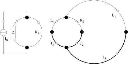
Figure 5: The flux-biased IBM qubit. The coil inductance $K_{4}$ can either be coupled to the main loop via a mutual inductance to $L_{1}$ or to the control loop via $L_{3}$.

The network graph ($N=7$ nodes, $B=15$ branches) shown in Fig. 5 has the following characteristics,

$${\bf F}_{CL}=\left(\begin{array}[]{r r}1&0\\ -1&1\\ 0&-1\end{array}\right), {\bf F}_{CZ}={\bf F}_{CB}={\bf 0}.$$ (205)

$${\bf F}_{KL}=\left(\begin{array}[]{r r}-1&1\\ 0&0\end{array}\right), {\bf F}_{KZ}=-{\bf F}_{KB}=\left(\begin{array}[]{r}0\\ -1\end{array}\right).\quad\quad$$ (210)

The structure of the inductance matrix depends on whether the external flux is coupled to the main loop or the control loop.

VIII.2.1 Main flux bias

For an external coil coupled to the main (larger) loop, the inductances are

$${\bf L}=\left(\begin{array}[]{c c}2L_{1}&0\\ 0&L_{3}\end{array}\right), {\bf L}_{K}=\left(\begin{array}[]{c c}L_{2}&0\\ 0&L_{c}\end{array}\right),$$ (215)

$${\bf L}_{LK}=\left(\begin{array}[]{c c}0&M\\ 0&0\end{array}\right),$$ (218)

where $L_{c}$ denotes the self-inductance of the coil and $M$ the mutual inductance between the coil and the main loop.

Since the system without external coupling is the same as for the current-biased version, the system Hamiltonian, i.e. the expressions for ${\bf M}_{0}$, ${\bf N}$, and $B_{0}$ are the same as for the current-biased circuit, Eqs. (178) and (182), with $L_{4}=L_{1}$. The spectral density is obtained via Eq. (108) and the result $K(\omega)=B_{0}/B_{\omega}$ where $B_{\omega}=2L_{1}(L_{2}+L_{3})(L_{c}+L_{z})-L_{3}M^{2}+L_{2}(L_{3}(L_{c}+L_{z}))-M^{2})$. For $\mu$ and ${\bf m}$ we find

$$\mu = M^{2}\frac{2(L_{2}^{2}+L_{2}L_{3}+L_{3}^{2})}{(L_{2}L_{3}+2L_{1}(L_{2}+L_{3}))^{2}},$$ (219)

$${\bf m} = \frac{1}{\sqrt{L_{2}^{2}+L_{3}^{2}+(L_{2}+L_{3})^{2}}}\left(\begin{array}[]{c}-(L_{2}+L_{3})\\ L_{3}\\ L_{2}\end{array}\right).\quad\quad$$ (223)

We study the following special cases of this result. If the control loop is symmetric, $L_{3}=L_{2}$, we obtain the simpler expressions

$$K(\omega) = \frac{4L_{1}+L_{2}}{4L_{1}(L_{c}+L_{z})+L_{2}(L_{c}+L_{z})-2M^{2}},\quad$$ (224)

$$\mu = \frac{6M^{2}}{(4L_{1}+L_{2})^{2}},\quad\quad{\bf m}=\frac{1}{\sqrt{6}}\left(\begin{array}[]{c}-2\\ 1\\ 1\end{array}\right).$$ (228)

If for a symmetric control loop, the control loop inductance is much smaller than the main loop inductance, i.e. for $L_{1}\gg L_{2}$, we find

$$K(\omega) = \frac{4L_{1}}{4L_{1}(L_{c}+L_{z})-2M^{2}}\approx\frac{i\omega}{Z(\omega)},$$ (229)

$$\mu = \frac{3M^{2}}{8L_{1}^{2}}.$$ (230)

The second approximation for $K(\omega)$ is suitable if $\omega\ll Z(\omega)/L_{c},Z(\omega)L_{1}/M^{2}$. The intuitive explanation for the result Eq. (228) is essentially the same as above for Eq. (201), with the difference that the inductively coupled current fluctuations couple oppositely to the Josephson junction in the main loop.

VIII.2.2 Control flux bias

An external coil coupled to the control (small) loop can be described by the inductances

$${\bf L}=\left(\!\begin{array}[]{c c}2L_{1}&0\\ 0&L_{3}\end{array}\!\right), {\bf L}_{K}=\left(\!\begin{array}[]{c c}L_{2}&-M/2\\ -M/2&L_{c}\end{array}\!\right),\quad\quad$$ (235)

$${\bf L}_{LK}=\left(\!\begin{array}[]{c c}0&0\\ 0&M/2\end{array}\!\right),$$ (238)

where $L_{c}$ is the self-inductance of the coil and $M$ is the total mutual inductance between the coil and the control loop. Again, the expressions for ${\bf M}_{0}$, ${\bf N}$, and $B_{0}$ are the same as for the current-biased circuit. We find $K(\omega)=B_{0}/B_{\omega}$ with $B_{\omega}=(-L_{3}M^{2}+8L_{1}(L_{2}(L_{c}+L_{z})+L_{3}(L_{c}+L_{z})-M^{2})+L_{2}(4L_{3}(L_{c}+L_{z})-M^{2}))/4$, and

$$\mu = M^{2}\frac{16L_{1}^{2}+L_{2}^{2}-L_{2}L_{3}+L_{3}^{2}+4L_{1}(L_{2}+L_{3})}{2(L_{2}L_{3}+2L_{1}(L_{2}+L_{3}))^{2}},$$

$${\bf m} = \frac{1}{\sqrt{(4L_{1}+L_{2})^{2}+(4L_{1}+L_{3})^{2}+(L_{2}-L_{3})^{2}}}\times$$ (243)

$$\times\left(\begin{array}[]{c}-L_{2}+L_{3}\\ -(4L_{1}+L_{3})\\ 4L_{1}+L_{2}\end{array}\right).$$

Since the bias current is shunted parallel to the external impedance, we find ${\bf S}=-\bar{\bf m}=-\sqrt{\mu}{\bf m}$. For a symmetric control loop, $L_{3}=L_{2}$, we obtain

$$K(\omega) = \frac{2L_{2}}{2L_{2}(L_{c}+L_{z})-M^{2}}\approx\frac{i\omega}{Z(\omega)},$$ (244)

$$\mu = \frac{M^{2}}{2L_{2}^{2}},\quad\quad{\bf m}=\frac{1}{\sqrt{2}}\left(\begin{array}[]{c}0\\ -1\\ 1\end{array}\right).$$ (248)

The second approximation for $K(\omega)$ is suitable if $\omega\ll Z(\omega)/L_{c},Z(\omega)L_{2}/M^{2}$.

The result Eq. (248) reflects the fact that in the symmetric case, $L_{3}=L_{2}$, a control flux bias only affects the superconducting phases in the control loop. The two phases are affected with the same magnitude of fluctuations, but with opposite sign.

IX The Delft qubit

As a further application of our theory, we study decoherence in a superconducting circuit studied experimentally as a candidate for a superconducting flux qubit in Refs. Mooij, ; Orlando, .

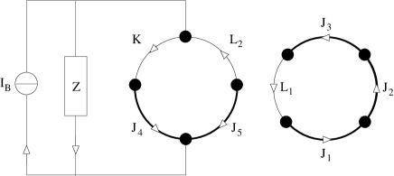
Figure 6: The graph representation of the Delft qubit. The “qubit” loop (right) involves three Josephson junctions $J_{i}$ (i=1,2,3; thick lines) and is inductively coupled to the SQUID (or read-out) loop (left) which comprises two junctions and can be current biased.

The circuit consists of a ring similar to a dc SQUID but with three junctions, see Fig. 6. For readout, a dc SQUID is inductively coupled to the three-junction (qubit) loop. The readout SQUID is current biased in order to find its critical current. The value of the critical current can then be used to determine the state of the qubit loop.

This circuit network graph characteristics of the Delft qubit are ($N=8$ nodes, $B=20$ branches),

$${\bf F}_{CL}=\left(\begin{array}[]{r r}-1&0\\ -1&0\\ -1&0\\ 0&-1\\ 0&1\end{array}\right), {\bf F}_{CZ}=-{\bf F}_{CB}=\left(\begin{array}[]{r}0\\ 0\\ 0\\ 1\\ 0\end{array}\right)\!,$$ (259)

$${\bf F}_{KL}=\left(\begin{array}[]{r r}0&-1\end{array}\right), {\bf F}_{KZ}=-{\bf F}_{KB}=\left(\begin{array}[]{r}1\end{array}\right)\!.\quad\quad$$ (262)

We use the following assignment for the inductances

$${\bf L}=\left(\!\begin{array}[]{c c}L&M_{R}\\ M_{R}&L_{R}\end{array}\!\right)\!,\,{\bf L}_{K}=\left(\!\begin{array}[]{c c}L_{L}\end{array}\!\right)\!,\,{\bf L}_{LK}=\left(\!\begin{array}[]{c}M_{L}\\ M^{\prime}\end{array}\!\right)\!,\,$$ (263)

where $L$ and $L^{\prime}=L_{L}+L_{R}$ are the self-inductances of the qubit and SQUID loops, respectively, and $M=M_{L}+M_{R}$ is the mutual inductance between the two loops. The self-inductance of the SQUID loop and the mutual inductance are divided into parts $L_{L}$ and $M_{L}$ corresponding to the left half of the SQUID loop and parts $L_{R}$ and $M_{R}$ corresponding to the right half of the SQUID loop. We introduce the following notations and conventions. The Josephson inductances of the five junctions are given by $L_{J,1}=L_{J,2}=L_{J}$ and $L_{J,3}=L_{J}/\beta$ for the three qubit junctions, and $L_{J;L,R}=L_{J}^{\prime}$ for the two SQUID junctions. The superconducting phase differences across the five junctions are denoted with ${\mbox{\boldmath$\varphi$}}=(\varphi_{1},\varphi_{2},\varphi_{3},\varphi_{L},\varphi_{R})$, and the capacitances of the five junctions are ${\bf C}={\rm diag}(C,C,C,C^{\prime},C^{\prime})$. The externally applied fluxes threading the qubit and SQUID loops are described by the vector ${\bf\Phi}_{x}=(\Phi_{x},\Phi_{x}^{\prime})$. In the symmetric case, $L_{L}=L_{R}=L^{\prime}/2$, $M_{L}=M_{R}=M/2$, we obtain

$${\bf M}_{0} = \frac{1}{LL^{\prime}-M^{2}}\left(\!\begin{array}[]{r r r r r}L^{\prime}&L^{\prime}&L^{\prime}&-M&M\\ L^{\prime}&L^{\prime}&L^{\prime}&-M&M\\ L^{\prime}&L^{\prime}&L^{\prime}&-M&M\\ -M&-M&-M&L&-L\\ M&M&M&-L&L\end{array}\!\right)\!,\quad\quad$$ (269)

$${\bf N} = \frac{1}{LL^{\prime}-M^{2}}\left(\begin{array}[]{r r}-L^{\prime}&M\\ -L^{\prime}&M\\ -L^{\prime}&M\\ M&-L\\ -M&L\end{array}\right)$$ (275)

for the Hamiltonian and

$$K(\omega)=\frac{i\omega}{Z(\omega)+i\omega L^{\prime}/4},$$ (276)

$\mu=1/2$, ${\bf m}=(0,0,0,1,1)/\sqrt{2}$, and ${\bf S}=-\sqrt{\mu}{\bf m}$.

Instead of quantizing the classical Hamiltonian Eq. (95), with Eqs. (269) and (275) we will linearize the dc SQUID in order to separate the degrees of freedom that become very massive under the influence of the external impedance from the other, light degrees of freedom. Subsequently, we will only quantize the light degrees of freedom, viewing the massive degrees of freedom as part of the environment.

IX.1 Linearization of the dc-SQUID

We start by linearizing the uncoupled ($M=0$) SQUID. The equations of motion for the SQUID are

$$\frac{C^{\prime}}{2}\left(\ddot{\varphi}_{L}-\ddot{\varphi}_{R}\right) = -\frac{1}{2L_{J}^{\prime}}\left(\sin\varphi_{L}-\sin\varphi_{R}\right)$$ (277)

$$-\frac{1}{L^{\prime}}\left(\varphi_{L}-\varphi_{R}-2\pi\frac{\Phi^{\prime}_{x}}{\Phi_{0}}\right),$$

$$\frac{C^{\prime}}{2}\left(\ddot{\varphi}_{L}+\ddot{\varphi}_{R}\right) = -\frac{1}{2L_{J}^{\prime}}\left(\sin\varphi_{L}+\sin\varphi_{R}\right)+\frac{2\pi}{\Phi_{0}}I_{B}$$ (278)

$$-\mu K*\left(\varphi_{L}+\varphi_{R}\right)(t).$$

Now we make the expansion

$$\varphi_{L,R}(t)=\bar{\varphi}_{L,R}+\delta\varphi_{L,R}(t),$$ (279)

where $\bar{\varphi}_{L,R}$ denotes the steady-state solution of the classical equations of motion Eqs. (277) and (278). We first find this steady-state solution in the absence of a bias current, $I_{B}=0$, using $L^{\prime}\ll L_{J}^{\prime}$ and assume $\Phi_{x}^{\prime}\neq\Phi_{0}/2$, with the result

$$\bar{\varphi}_{L}^{(0)}=-\bar{\varphi}_{R}^{(0)}=\pi\frac{\Phi_{x}^{\prime}}{\Phi_{0}}.$$ (280)

Next, we allow a finite but small bias current $I_{B}\ll I_{c}^{\prime}=\Phi_{0}/2\pi L_{J}^{\prime}$, and with $\bar{\varphi}_{L,R}=\bar{\varphi}_{L,R}^{(0)}+\delta\bar{\varphi}_{L,R}$ we find

$$\delta\bar{\varphi}_{L}=\delta\bar{\varphi}_{R}=\pi\frac{L_{J}^{\prime}I_{B}}{\Phi_{0}\cos(\pi\Phi_{x}^{\prime}/\Phi_{0})}.$$ (281)

Starting from the steady-state solution, we can now derive the linearized SQUID dynamics $\delta\varphi(t)$. We assume that the external impedance $Z(\omega)$ contains a sizable shunt capacitance $C_{\rm sh}\gg C^{\prime}$ and that $\omega\ll 1/\sqrt{L^{\prime}C^{\prime}}$ ($\approx 1500\,{\rm GHz}$ for typical values $C^{\prime}=1\,{\rm fF}$, $L^{\prime}=10\,{\rm pH}$). Under these assumptions, the effect of the external impedance $Z\approx 1/i\omega C_{\rm sh}$ is to make the coordinate $\varphi_{L}+\varphi_{R}$ very “massive”, i.e.,

$$K(\omega)\approx\frac{i\omega C_{\rm sh}}{4},\quad\quad\int_{0}^{t}K(t-t^{\prime})\varphi_{+}(t^{\prime})\approx\frac{C_{\rm sh}}{4}\ddot{\varphi}_{+}(t),$$ (282)

the “mass” being $C^{\prime}+C_{\rm sh}/4\approx C_{\rm sh}/4$. In order to eliminate $\varphi_{L}+\varphi_{R}$ from the classical equations of motion, we introduce $\varphi_{\pm}=\varphi_{L}\pm\varphi_{R}$ and expand Eqs. (277) and (278) about the steady-state solution, $\varphi_{\pm}=\bar{\varphi}_{\pm}+\delta\varphi_{\pm}$,

$$\left[\omega^{2}\frac{C^{\prime}}{2}\!+\!\left(\!\!\begin{array}[]{c c}\frac{c_{+}}{2L_{J}^{\prime}}\!+\!\frac{1}{L^{\prime}}&\frac{c_{-}}{2L_{J}^{\prime}}\\ \frac{c_{-}}{2L_{J}^{\prime}}&\frac{c_{+}}{2L_{J}^{\prime}}\!+\!\mu K(\omega)\end{array}\!\!\right)\right]\!\left(\!\begin{array}[]{c}\delta\varphi_{-}(\omega)\\ \delta\varphi_{+}(\omega)\end{array}\!\right)\!=\!\left(\!\begin{array}[]{c}0\\ 0\end{array}\!\right)\!,\\$$

where we have used the steady-state solution to define

$$c_{+} \equiv \cos\bar{\varphi}_{L}+\cos\bar{\varphi}_{R}=2\cos\pi\frac{\Phi_{x}^{\prime}}{\Phi_{0}},$$ (283)

$$c_{-} \equiv \cos\bar{\varphi}_{L}-\cos\bar{\varphi}_{R}=-2\pi\frac{L_{J}^{\prime}I_{B}}{\Phi_{0}}\tan\pi\frac{\Phi_{x}^{\prime}}{\Phi_{0}}.$$ (284)

Neglecting $C^{\prime}\ll C_{\rm sh}$ in the equation of motion for $\delta\varphi_{+}$, we can solve for $\delta\varphi_{+}$ (neglecting higher powers of $I_{B}$),

$$\delta\varphi_{+}(\omega)=-c_{-}\left(c_{+}+\frac{i\omega L_{J}^{\prime}/2}{Z(\omega)+i\omega L^{\prime}/4}\right)^{-1}\delta\varphi_{-}(\omega).$$ (285)

Substituting this back into Eq. (IX.1), we obtain the following damping term in the equations of motion for $\delta\varphi_{-}$

$$\frac{c_{-}}{2L_{J}^{\prime}}\delta\varphi_{+}(\omega)=-\frac{i\omega}{\tilde{Z}(\omega)}\delta\varphi_{-}(\omega),$$ (286)

with the effective SQUID inductance $\tilde{L}_{J}=L_{J}^{\prime}/4\cos(\pi\Phi_{x}/\Phi_{0})=L_{J}^{\prime}/2c_{+}$ and the effective external impedance

$$\tilde{Z}(\omega)=-\frac{\omega^{2}L_{J}^{\prime 2}}{Z_{t}(\omega)}\left(\frac{I_{B}}{I_{c}^{\prime}}\tan\pi\frac{\Phi_{x}^{\prime}}{\Phi_{0}}\right)^{-2},$$ (287)

where $I_{c}^{\prime}$ is the critical current of the SQUID junctions and the total impedance (heavy SQUID degree of freedom in parallel with external impedance $Z$) is defined through

$$Z_{t}(\omega)=\left(\frac{1}{i\omega\tilde{L}_{J}}+\frac{1}{Z(\omega)+i\omega L^{\prime}/4}\right)^{-1}.$$ (288)

The effective external impedance $\tilde{Z}$ is much larger than $\omega L_{J}^{\prime}$ for $I_{B}\ll I_{c}^{\prime}$ or for $\sin\pi\Phi_{x}^{\prime}/\Phi_{0}\approx 0$. Thus, unlike $\delta\varphi_{+}$, the remaining degrees of freedom (including $\delta\varphi_{-}$) are weakly affected by the effective external impedance and will be described as quantum mechanical degrees of freedom.

IX.2 Description of the light degrees of freedom

After having eliminated one degree of freedom from the SQUID, the remaining four degrees of freedom ${\mbox{\boldmath$\varphi$}}=(\varphi_{1},\varphi_{2},\varphi_{3},\delta\varphi_{-})$ will are now described by the Hamiltonian Eq. (95) with the capacitances ${\bf C}={\rm diag}(C,C,C,C^{\prime}/2)$, the Josephson effective inductances ${\bf L}_{J}^{-1}={\rm diag}(L_{J}^{-1},L_{J}^{-1},\beta L_{J}^{-1},0)$, and

$${\bf M}_{0} = \frac{1}{LL^{\prime}-M^{2}}\left(\begin{array}[]{r r r r}L^{\prime}&L^{\prime}&L^{\prime}&-M\\ L^{\prime}&L^{\prime}&L^{\prime}&-M\\ L^{\prime}&L^{\prime}&L^{\prime}&-M\\ -M&-M&-M&L\end{array}\right)$$ (298)

$$+\frac{1}{\tilde{L}_{J}}\left(\begin{array}[]{r r r r}0&0&0&0\\ 0&0&0&0\\ 0&0&0&0\\ 0&0&0&1\end{array}\right),$$

$${\bf N} = \frac{1}{LL^{\prime}-M^{2}}\left(\begin{array}[]{r r r r r}-L^{\prime}&M\\ -L^{\prime}&M\\ -L^{\prime}&M\\ M&-L\end{array}\right).$$ (303)

Since the part of the circuit that was coupled to the bias current is described by $\tilde{Z}$, there is no coupling to a bias current left, ${\bf S}=0$. By inspecting Eq. (286), we find ${\bf m}=(0,0,0,1)$, $\mu=1$, and

$$K(\omega)=\frac{i\omega}{\tilde{Z}(\omega)}.$$ (304)

The results Eqs. (298)–(304) for the reduced system can also be obtained from the circuit drawn in Fig. 7 with $C_{4}=C^{\prime}/2$ and the inductance matrix

$${\bf L}=\left(\begin{array}[]{c c c}L&M&0\\ M&L^{\prime}&0\\ 0&0&\tilde{L}_{J}\end{array}\right).$$ (305)

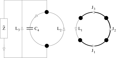
Figure 7: Circuit representation of the Delft qubit with a linearized SQUID. The analysis is simplified due to the absence of tree inductors (K).

Using Eqs. (146), (147), (304), and (287), we obtain

$$\frac{1}{T_{1}} = \left(\frac{\Delta}{\omega_{01}}\right)^{2}\left(\frac{\Phi_{0}}{2\pi}\right)^{2}|{\bf m}\cdot\Delta{\mbox{\boldmath$\varphi$}}|^{2}\frac{1}{\omega_{01}}{\rm Re}Z_{t}(\omega_{01})\times$$ (306)

$$\times\left(\frac{2\pi I_{B}}{\Phi_{0}}\tan\pi\frac{\Phi_{x}^{\prime}}{\Phi_{0}}\right)^{2}\coth\frac{\omega_{01}}{2k_{B}T},$$

$$\frac{1}{T_{\phi}} = \left(\frac{\epsilon}{\omega_{01}}\right)^{2}\left(\frac{\Phi_{0}}{2\pi}\right)^{2}|{\bf m}\cdot\Delta{\mbox{\boldmath$\varphi$}}|^{2}{\rm Re}Z_{t}(0)\times$$ (307)

$$\times\left(\frac{2\pi I_{B}}{\Phi_{0}}\tan\pi\frac{\Phi_{x}^{\prime}}{\Phi_{0}}\right)^{2}2k_{B}T.$$

We make the approximation that the SQUID is completely classical; solving the classical equation of motion Eq. (76) for $\delta\varphi_{-}$ using Eq. (298), we obtain the stationary classical solution for $\delta\varphi_{-}$ (with $L^{\prime},L\ll L_{J}^{\prime},\tilde{L}_{J}$),

$$\delta\varphi_{-}=-\frac{2\pi}{\Phi_{0}}\left(MI+\Phi_{x}^{\prime}\right),$$ (308)

where we have used that $\sum_{i}\varphi_{i}=-2\pi\Phi/\Phi_{0}$, where $\Phi$ is the flux threading the qubit loop, and $\Phi-\Phi_{x}=LI$, where $I$ is the current circulating in the qubit loop. The difference between the two minima $\varphi$ (localized states $|0\rangle$ and $|1\rangle$) is then ($\Phi_{x}$ is constant)

$${\bf m}\cdot\Delta{\mbox{\boldmath$\varphi$}}=\Delta\delta\varphi_{-}\approx-\frac{2\pi}{\Phi_{0}}M(I_{L}-I_{R}),$$ (309)

and since $I_{L}=-I_{R}\equiv I$,

$${\bf m}\cdot\Delta{\mbox{\boldmath$\varphi$}}\approx-2\frac{2\pi}{\Phi_{0}}MI.$$ (310)

Substituting the above result into Eqs. (306) and (307), we obtain

$$\frac{1}{T_{1}} = 4\left(\frac{\Delta}{\omega_{01}}\right)^{2}I_{B}^{2}\frac{1}{\omega_{01}}\left(\frac{2\pi MI}{\Phi_{0}}\tan\pi\frac{\Phi_{x}^{\prime}}{\Phi_{0}}\right)^{2}\times$$ (311)

$$\times{\rm Re}Z_{t}(\omega_{01})\coth\frac{\omega_{01}}{2k_{B}T}$$

$$\frac{1}{T_{\phi}} = 4\left(\frac{\epsilon}{\omega_{01}}\right)^{2}I_{B}^{2}\frac{1}{\omega_{01}}\left(\frac{2\pi MI}{\Phi_{0}}\tan\pi\frac{\Phi_{x}^{\prime}}{\Phi_{0}}\right)^{2}\times$$ (312)

$$\times{\rm Re}Z_{t}(0)2k_{B}T,$$

which agrees with earlier results WWHM . We also obtain an estimate for the leakage rate from Eq. (171),

$$\frac{1}{T_{L}}=\left(\frac{\delta}{\eta}\right)^{2}\!\!\!I_{B}^{2}\frac{1}{\eta}\!\!\left(\frac{2\pi MI}{\Phi_{0}}\tan\pi\frac{\Phi_{x}^{\prime}}{\Phi_{0}}\right)^{2}\!\!\!{\rm Re}Z_{t}(\eta)\coth\frac{\eta}{2k_{B}T}.$$ (313)

IX.3 Asymmetric SQUID

Up to now we have assumed that the SQUID ring in the Delft qubit is symmetric in two senses; namely that both the self-inductances of the left and right halves of the ring are identical and the critical currents of the Josephson junctions in the left and right halves of the SQUID ring are identical. Both symmetries are certainly broken to some degree in real physical systems. Below, we study both cases, i.e. the case where the self-inductances of the left and right halves of the ring are different (geometrical asymmetry) and the case where the two critical currents are different (Junction asymmetry).

IX.3.1 Geometric asymmetry

We analyze the Delft qubit again with the inductance matrix Eq. (263) and the asymmetric inductances

$$M_{L} = \left(1+\frac{\alpha}{2}\right)\frac{M}{2},\quad M_{R}=\left(1-\frac{\alpha}{2}\right)\frac{M}{2},$$ (314)

$$L_{L} = \left(1+\frac{\alpha}{2}\right)\frac{L^{\prime}}{2},\quad L_{R}=\left(1-\frac{\alpha}{2}\right)\frac{L^{\prime}}{2},$$ (315)

where $M_{L}+M_{R}=M$ and $L_{L}+L_{R}=L^{\prime}$. By linearizing the SQUID, we obtain the result

$$\tilde{Z}(\omega)=-\frac{\omega^{2}L_{J}^{\prime 2}}{Z_{t}(\omega)}\left[\left(\frac{I_{B}}{I_{c}^{\prime}}\tan\pi\frac{\Phi_{x}^{\prime}}{\Phi_{0}}\right)^{2}+\alpha\frac{I_{B}}{I_{c}^{\prime}}\sin\pi\frac{\Phi_{x}^{\prime}}{\Phi_{0}}\right]^{-1}.$$ (316)

This result implies that if $\alpha\gg I_{B}/I_{c}^{\prime}$, the decoherence rates scale as $\alpha I_{B}/I_{c}^{\prime}$ instead of $(I_{B}/I_{c}^{\prime})^{2}$ for $\alpha\ll I_{B}/I_{c}^{\prime}$. Therefore, for very asymmetric loops, $\alpha\gg I_{B}/I_{c}^{\prime}$, moderate bias currents can already cause large decoherence effects.

IX.3.2 Junction asymmetry

For asymmetric critical currents, or, equivalently, asymmetric effective Josephson inductances,

$$L_{J;L,R}^{\prime}=L_{J}^{\prime}(1\pm\gamma/2),$$ (317)

we repeat the linearization of the SQUID keeping contributions of lowest order in $\gamma$. Setting $I_{B}=0$, we obtain

$$\frac{1}{L_{J;L,R}}\approx\frac{1}{L_{J}}\left(1\mp\frac{\gamma}{2}\right)+O(\gamma^{2}).$$ (318)

The steady state of the SQUID is then determined by the following equations,

$$\bar{\varphi}_{L}-\bar{\varphi}_{R}=-2\pi\frac{\Phi_{x}^{\prime}}{\Phi_{0}},$$ (319)

$$\left(1-\frac{\gamma}{2}\right)\sin\bar{\varphi}_{L}+\left(1+\frac{\gamma}{2}\right)\sin\bar{\varphi}_{R} = 0.$$ (320)

We make the ansatz

$$\bar{\varphi}_{L,R}=\mp\pi\frac{\Phi_{x}^{\prime}}{\Phi_{0}}+\gamma q,$$ (321)

and obtain the result $q=-\tan(\pi\Phi_{x}^{\prime}/\Phi_{0})/2$, and finally,

$$\bar{\varphi}_{L,R}=\mp\pi\frac{\Phi_{x}^{\prime}}{\Phi_{0}}-\frac{\gamma}{2}\tan\pi\frac{\Phi_{x}^{\prime}}{\Phi_{0}}.$$ (322)

Comparing this to Eq. (281), we see that in order to obtain the Redfield tensor and the decoherence rates at zero bias current in the presence of a junction asymmetry $\gamma$, we simply have to make the substitution

$$\frac{I_{B}}{I_{c}^{\prime}}\longrightarrow\gamma\sin\pi\frac{\Phi_{x}^{\prime}}{\Phi_{0}}.$$ (323)

Typical values for the junction asymmetry due to processing inaccuracies are fairly large, $\gamma\approx 10\%$. The effect of a junction asymmetry is more severe than the effect of a geometrical asymmetry because for asymmetric junctions, decoherence occurs even for zero bias current $I_{B}=0$.

Appendix A Symmetry of ${\bf M}_{0}$

In this Appendix, we prove that the matrix ${\bf M}_{0}$ defined in Eq. (77) is always symmetric, ${\bf M}_{0}^{T}={\bf M}_{0}$. This property is required in order to find a potential $U({\mbox{\boldmath$\varphi$}})$ generating the force term $-{\bf M}_{0}{\mbox{\boldmath$\varphi$}}$ in the equation of motion. We write ${\bf M}_{0}={\bf F}_{CL}{\bf V}{\bf W}^{-1}{\bf F}_{CL}^{T}$ with

$${\bf V} = \tilde{\bf L}_{L}^{-1}\bar{\bf L}=\openone_{L}+{\bf X}\tilde{\bf L}_{K}\bar{\bf F}_{KL},$$ (324)

$${\bf W} = {\bf L}_{LL}=\bar{\bf L}+{\bf F}_{KL}^{T}\tilde{\bf L}_{K}\bar{\bf F}_{KL},$$ (325)

with the off-diagonal block of ${\bf L}_{\rm t}$ from Eq. (42),

$${\bf X} = -{\bf L}^{-1}{\bf L}_{LK}\bar{\bf L}_{K}^{-1},$$ (326)

$${\bf X}^{T} = -{\bf L}_{K}^{-1}{\bf L}_{LK}^{T}\bar{\bf L}^{-1},$$ (327)

and show that ${\bf V}{\bf W}^{-1}$ is symmetric, thus proving that ${\bf M}_{0}$ is symmetric. Note that in Eq. (327) we have used that ${\bf L}_{\rm t}$ is symmetric. As a first step of our proof, we note that the symmetry of ${\bf V}{\bf W}^{-1}$,

$$({\bf V}{\bf W}^{-1})^{T}\equiv({\bf W}^{T})^{-1}{\bf V}^{T}={\bf V}{\bf W}^{-1},$$ (328)

is equivalent to the relation

$${\bf V}^{T}{\bf W}={\bf W}^{T}{\bf V}.$$ (329)

As a second step, we use Eq. (53) to show

$${\bf V}^{T}{\bf W}-{\bf W}^{T}{\bf V}=\bar{\bf F}_{KL}^{T}\tilde{\bf L}_{K}^{T}\left({\bf Y}-{\bf Y}^{T}\right)\tilde{\bf L}_{K}\bar{\bf F}_{KL},$$ (330)

where ${\bf Y}=(\tilde{\bf L}_{K}^{T})^{-1}-{\bf F}_{KL}{\bf X}$. The third and last step of the proof is to show that ${\bf Y}$ is symmetric, i.e. ${\bf Y}={\bf Y}^{T}$. For this, we rewrite Eqs. (52) and (53) as

$$\tilde{\bf L}_{K} = (\openone_{K}-{\bf L}_{K}\bar{\bf F}_{KL}{\bf X})^{-1}{\bf L}_{K},$$ (331)

$$\bar{\bf F}_{KL} = {\bf F}_{KL}-{\bf X}^{T}\bar{\bf L}.$$ (332)

Using these relations, we can show that ${\bf Y}={\bf L}_{K}^{-1}+{\bf X}^{T}\bar{\bf L}{\bf X}$ which is manifestly symmetric. This concludes the proof that ${\bf M}_{0}$ is symmetric.

Appendix B Symmetry of ${\bf M}_{d}$

From Eqs. (III.4), (74), and (75), we obtain hEq. (76) with

$${\bf M}_{d}(\omega) = {\bf F}_{CL}\left(\tilde{\bf L}_{L}^{-1}\bar{\bf L}{\bf L}_{LL}^{-1}{\bf L}_{LZ}-{\bf L}^{-1}{\bf L}_{LK}\bar{\bf L}_{K}^{-1}\tilde{\bf L}_{K}{\bf F}_{KZ}\right)\bar{\bf L}_{Z}^{-1}(\omega){\bf L}_{ZL}{\bf L}_{LL}^{-1}{\bf F}_{CL}^{T}$$

$$+{\bf F}_{CZ}\bar{\bf L}_{Z}^{-1}(\omega)\left({\bf F}_{CZ}^{T}-{\bf L}_{ZL}{\bf L}_{LL}^{-1}(\omega){\bf F}_{CL}^{T}\right)+{\bf F}_{CL}\left({\bf L}^{-1}{\bf L}_{LK}\bar{\bf L}_{K}^{-1}\tilde{\bf L}_{K}{\bf F}_{KZ}-\tilde{\bf L}_{L}^{-1}\bar{\bf L}{\bf L}_{LL}^{-1}{\bf L}_{LZ}\right)\bar{\bf L}_{Z}^{-1}(\omega){\bf F}_{CZ}^{T},$$

where we have used the identity $\bar{\bf L}_{L}^{-1}(\omega){\bf L}_{LZ}{\bf L}_{ZZ}^{-1}(\omega)={\bf L}_{LL}^{-1}{\bf L}_{LZ}\bar{\bf L}_{Z}^{-1}(\omega)$. This expression is a quadratic form in ${\bf F}_{CL}$ and ${\bf F}_{CZ}$,

$${\bf M}_{d}=\left(\begin{array}[]{r r}\!\!{\bf F}_{CL}\!&\!{\bf F}_{CZ}\!\!\end{array}\right)\left(\begin{array}[]{r r}{\bf A}\bar{\bf L}_{Z}^{-1}{\bf B}&{\bf A}\bar{\bf L}_{Z}^{-1}\\ \bar{\bf L}_{Z}^{-1}{\bf B}&\bar{\bf L}_{Z}^{-1}\end{array}\right)\left(\begin{array}[]{r}{\bf F}_{CL}^{T}\\ {\bf F}_{CZ}^{T}\end{array}\right),$$ (334)

with the definitions

$${\bf A} = -\tilde{\bf L}_{L}^{-1}\bar{\bf L}{\bf L}_{LL}^{-1}{\bf L}_{LZ}+{\bf L}^{-1}{\bf L}_{LK}\bar{\bf L}_{K}^{-1}\tilde{\bf L}_{K}{\bf F}_{KZ},$$ (335)

$${\bf B} = -{\bf L}_{ZL}{\bf L}_{LL}^{-1}=-{\bf F}_{KZ}^{T}\tilde{\bf L}_{K}\bar{\bf F}_{KL}{\bf L}_{LL}^{-1}.$$ (336)

Next, we show that ${\bf M}_{d}$ must be symmetric, ${\bf M}_{d}^{T}={\bf M}_{d}$, and therefore $\bar{\bf L}_{Z}^{T}=\bar{\bf L}_{Z}$ and ${\bf A}={\bf B}^{T}$.

The argument for the symmetry of ${\bf M}_{d}$ is as follows. We consider a generalized model in which the external impedances $Z$ and the linear inductances $L$ and $K$ are treated on an equal footing. For this purpose, we allow mutual impedances (generalized mutual inductances) between $Z$ and $K$ and include $Z$ into $L$ by allowing frequency dependent linear inductances and writing $L_{Z}(\omega)=Z(\omega)/i\omega$. This leaves us with the following types of circuit elements; tree elements are either capacitors $C$ or linear impedances $K$ where ${\bf L}_{K}(\omega)={\bf Z}_{K}(\omega)/i\omega$, branch elements are Josephson junctions (non-linear inductors) $J$, linear impedances $L$ where ${\bf L}(\omega)={\bf Z}_{L}(\omega)/i\omega$, and external bias currents $B$. In addition to this, there can be frequency-dependent linear mutual impedances ${\bf Z}_{LK}(\omega)$, where ${\bf L}_{LK}(\omega)={\bf Z}_{LK}(\omega)/i\omega$, between the $L$ and $K$ branches. The equation of motion (76) can now be derived exactly as before, but in the frequency domain, the result being Eq. (76) without the ${\bf M}_{d}(\omega)$ term, since there are no $Z$ branches. These new equations include dissipation which is described by the (now frequency-dependent) ${\bf M}_{0}^{\prime}(\omega)$, the prime distinguishing it from the “ordinary” ${\bf M}_{0}$ (see above). The matrix ${\bf M}_{0}^{\prime}$ is formally identical to ${\bf M}_{0}$, up to frequency dependencies which are irrelevant for the symmetry of the matrix. We have shown in Appendix A that ${\bf M}_{0}^{T}={\bf M}_{0}$; this proof also goes through for ${\bf M}_{0}^{\prime}$, thus ${\bf M}_{0}^{\prime T}={\bf M}_{0}^{\prime}$. Since ${\bf M}_{0}^{\prime}(\omega)={\bf M}_{0}+{\bf M}_{d}(\omega)$ and both ${\bf M}_{0}$ and ${\bf M}_{0}^{\prime}$ are symmetric, we conclude that also ${\bf M}_{d}^{T}={\bf M}_{d}$. Introducing $\bar{\bf m}={\bf F}_{CL}+{\bf F}_{CZ}{\bf A}={\bf F}_{CL}+{\bf F}_{CZ}{\bf B}^{T}$, we can now write ${\bf M}_{d}$ in the form given in Eqs. (79) and (80).

References

• (1) E. Schrödinger, Die Naturwissenschaften 23, 807 (1935).
• (2) R. F. Voss and R. A. Webb, Phys. Rev. Lett. 47, 265 (1981).
• (3) J. M. Martinis, M. H. Devoret, and J. Clarke, Phys. Rev. B 35, 4682 (1987).
• (4) J. Clarke, A. N. Cleland, M. H. Devoret, D. Esteve, and J. M. Martinis, Science 239, 992 (1988).
• (5) R. Rouse, S. Han, and J. E. Lukens, Phys. Rev. Lett. 75, 1614 (1995).
• (6) Y. Makhlin, G. Schön, and A. Shnirman, Rev. Mod. Phys. 73, 357 (2001).
• (7) A. O. Caldeira and A. J. Leggett, Ann. Phys. (N.Y.) 143, 374 (1983).
• (8) M. A. Nielsen and I. L. Chuang, Quantum Computation and Quantum Information (Cambridge University Press, 2000).
• (9) J. M. Martinis, S. Nam, J. Aumentado, and C. Urbina, Phys. Rev. Lett. 89, 117901 (2002).
• (10) L. Tian, L. S. Levitov, J. E. Mooij, T. P. Orlando, C. H. van der Wal, S. Lloyd, in Quantum Mesoscopic Phenomena and Mesoscopic Devices in Microelectronics, I. O. Kulik, R. Ellialtioglu, eds. (Kluwer, Dordrecht, 2000), pp. 429-438; cond-mat/9910062.
• (11) L. Tian, S. Lloyd, and T. P. Orlando, Phys. Rev. B 65, 144516 (2002).
• (12) C. H. van der Wal, F. K. Wilhelm, C. J. P. M. Harmans, and J. E. Mooij, Eur. Phys. J. B 31, 111 (2003).
• (13) F. K. Wilhelm, M. J. Storcz, C. H. van der Wal, C. J. P. M. Harmans, and J. E. Mooij, Adv. Solid State Phys. 43, 763 (2003).
• (14) J. E. Mooij, T. P. Orlando, L. Levitov, L. Tian, C. H. van der Wal, S. Lloyd, Science 285, 1036 (1999).
• (15) T. P. Orlando, J. E. Mooij, L. Tian, C. H. van der Wal, L. S. Levitov, S. Lloyd, J. J. Mazo, Phys. Rev. B 60, 15398 (1999).
• (16) C. H. van der Wal, A. C. J. ter Har, F. K. Wilhelm, R. N. Schouten, C. J. P. M. Harmans, T. P. Orlando, S. Lloyd, and J. E. Mooij, Science 290, 773 (2000).
• (17) I. Chiorescu, Y. Nakamura, C. J. P. M. Harmans, J. E. Mooij, Science 299, 1869 (2003).
• (18) J. R. Friedman, V. Patel, W. Chen, S. K. Tolpygo, and J. E. Lukens, Nature 406, 43 (2000).
• (19) R. Koch, J. Kirtley, J. Rozen, J. Sun, G. Keefe, F. Milliken, C. Tsuei, D. DiVincenzo, Bull. Am. Phys. Soc. 48, 367 (2003).
• (20) B. Yurke and J. S. Denker, Phys. Rev. A 29, 1419 (1984).
• (21) B. Yurke, J. Opt. Soc. Am. B 4, 1557 (1987).
• (22) M. J. Werner and P. D. Drummond, Phys. Rev. A 43, 6414 (1991).
• (23) D. Esteve, M. H. Devoret, and J. M. Martinis, Phys. Rev. B 34, 158 (1986).
• (24) M. H. Devoret, p. 351 in Quantum fluctuations, lecture notes of the 1995 Les Houches summer school, eds. S. Reynaud, E. Giacobino, and J. Zinn-Justin (Elsevier, The Netherlands, 1997).
• (25) Yu. V. Nazarov and D. A. Bagrets, Phys. Rev. Lett. 88, 196801 (2002).
• (26) A. J. Leggett, S. Chakravarty, A. T. Dorsey, M. P. A. Fisher, A. Garg, and W. Zwerger, Rev. Mod. Phys. 59, 1 (1987).
• (27) U. Weiss, Quantum Dissipative Systems, 2nd ed. (World Scientific, 1999).
• (28) B. Peikari, Fundamentals of Network Analysis and Synthesis, Prentice-Hall (Englewood Cliffs, NJ, 1974).
• (29) A. G. Redfield, IBM J. Res. Develop. 1, 19 (1957).
• (30) M. Celio and D. Loss, Physica A 158, 769 (1989).