Multifractal Properties of Price Fluctuations
of Stocks and
Commodities
Abstract
We analyze daily prices of 29 commodities and 2449 stocks, each over a period of years. We find that the price fluctuations for commodities have a significantly broader multifractal spectrum than for stocks. We also propose that multifractal properties of both stocks and commodities can be attributed mainly to the broad probability distribution of price fluctuations and secondarily to their temporal organization. Furthermore, we propose that, for commodities, stronger higher order correlations in price fluctuations result in broader multifractal spectra.
pacs:
PACS numbers: 87.10.+e, 87.80.+s, 87.90.+yThe study of economic markets has recently become an area of active research for physicists [1], in part because of the large amount of data that can be accessed for statistical analysis. Markets are complex systems for which the variables characterizing the state of the system—e.g., the price of the goods, the number of trades, and the number of agents, are easily quantified. These variables serve as fundamental examples of scale invariant behavior—the scaling laws are valid for time scales from seconds to decades.
Much interest has concentrated on stocks, where a number of empirical findings have been established, such as [2] (i) the distribution of price changes is approximately symmetric and decays with power law tails with an exponent for the probability density function; (ii) the price changes are exponentially (short-range) correlated while the absolute values of price changes (“volatility”) are power-law (long-range) correlated.
Unlike stock and foreign exchange markets, commodity markets have received little attention. Recently, it was found [3] that commodity markets have qualitative features similar to those of the stock market. This similarity is intriguing because the commodity market has special features such as: (i) most commodities require storage; (ii) most commodities require transportation to bring them to the market from where they are produced; and (iii) it is plausible that commodities may exhibit a slower response to change in demand because the price depends on the supply of the actual object.
The multifractal (MF) spectrum [4] reflects the -point correlations [5] and thus provides more information about the temporal organization of price fluctuations than 2-point correlations. Previous work reports a broad MF spectrum of stock indices and foreign exchange markets [6, 7, 8, 9, 10, 11, 12]. Two recent models [13, 14] explain the observed MF properties by assuming that price changes are the product of two stochastic variables, one being uncorrelated and normally distributed and the other being correlated and log-normally distributed. The price changes predicted by these models do not have the power law probability distribution [2, 3] observed empirically, and thus shuffling the price changes significantly narrows the MF spectrum.
Here we show that the MF properties of commodities and stocks result partly from the temporal organization and partly from the power law distribution of price fluctuations. We also conjecture that it is feature (iii) of commodity markets that leads to a broader MF spectrum of commodities compared to stocks.
We define the normalized price fluctuation (“return”) as
| (1) |
where here day, is the price, and is the standard deviation of over the duration of the time series (typically 15 years). We use the multifractal detrended fluctuation analysis (MF-DFA) method [15] to study the MF properties of the returns for stocks and commodities. Following [15], given a time series we execute the following steps: (i) Calculate the profile; , where is the length of the time series, and is the mean. (ii) Divide into segments. (iii) Calculate the local trend for segments by least square polynomial fit. (iv) Determine the mean square fluctuation in each segment . (v) Evaluate . The scaling function of moment , [15] follows scaling law
| (2) |
Negative values weight more small fluctuations, while positive values of give more weight to large fluctuations.
When the contribution of the small fluctuations is comparable to the contribution of the large fluctuations, the series is monofractal and where is the Hurst exponent. If nonlinearly depends on , the series is MF. The Legendre transform of is
| (3) |
Monofractal series have only one value of , unlike MF series which have a distribution of values.
We analyze a database consisting of daily prices of 29 commodities [16] and 2449 stocks [17] spread over time periods ranging from 10 to 30 years (the average period is 15 years). Figure 1 shows the price of a typical commodity, corn, and a typical stock, IBM, and their corresponding returns. One striking difference between the commodity and the stock is that the commodity returns are more “clustered” into patches of small and large fluctuations. This feature is not reflected in the distribution and the autocorrelation function of the price fluctuations [3].
To emphasize the clustering of commodities, we shuffle the returns by randomly exchanging pairs, a procedure that preserves the distribution of the returns but destroys any temporal correlations. Specifically, the shuffling procedure consists of the following steps
-
(i)
Generate pairs of random integer numbers (with ) where is the total length of the time series to be shuffled.
-
(ii)
Interchange entries and .
-
(iii)
Repeat steps (i) and (ii) for steps. (This step ensures that ordering of entries in the time series is fully shuffled.)
To avoid systematic errors caused by the random number generators, the shuffling procedure is repeated with different random number seeds for each of the 2449 stocks and 29 commodities. The shuffled commodity series of necessity loses its clustering [18] [Fig. 1(e)]. On the other hand, the shuffled stock series resembles the original one.
First we compare the 2-point correlations using DFA [19] of the shuffled and the unshuffled returns for commodities and stocks (Fig. 2). Both corn (and all other commodities analyzed) and IBM (and all other stocks analyzed) have returns uncorrelated for time scales larger than one day [2, 3]. Thus, studying the 2-point correlations is not sufficient to uncover the clustering of the commodity returns.
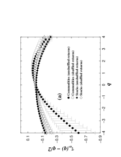
Next, we analyze the MF properties of the returns of stocks and commodities. Figure 3(a) displays separately the averages
| (4) |
for commodities, and for stocks. Note that (i) the scaling exponents, for commodities and stocks significantly differ, whereas are similar, suggesting that commodities are similar to stocks for the large fluctuations and they differ for the small fluctuations [20]; (ii) we observe that after shuffling the returns, for stocks hardly changes for , but for commodities changes and becomes comparable to stocks for the entire range of [21].
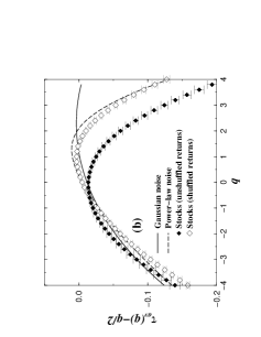
In order to study the contribution of the power law tails of the returns on the MF spectrum we generate surrogate data sets (i) with a normal distribution and (ii) with power law tails with (as is observed empirically [2, 3]). Figure 3(b) displays averaged over 2449 realizations of surrogate data, each with 3000 data points. The of the surrogate power law distributed data is very close to the of stocks after shuffling. This indicates that a significant part of the spectrum of stocks and commodities comes from the power law distribution of the returns. Note that there is a small difference in of stocks before and after shuffling, indicating that the power-law distribution of the returns is not the only source of multifractality but that there is also a relatively small contribution due to temporal organization of returns. For commodities this temporal organization is more dominant.
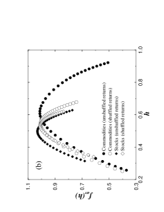
Figure 4 displays the MF spectrum of the unshuffled and shuffled returns for commodities and stocks. The temporal organization of commodity returns is reflected in the fact that the MF spectrum for unshuffled commodities is broader than for shuffled commodities and stocks.
Demand fluctuations drive price fluctuations, and it is plausible that stocks respond more quickly than commodities to demand changes. Stochastic perturbations, together with the immediate price response to demand changes, may weaken the existing higher order temporal organization, which may be the reason for less clustering for stocks (Fig. 1). Commodities, on the other hand, have a slower response. Thus, small or short-time perturbations are “felt” less by commodities than by stocks. This scenario is consistent with the appearance of patches of small commodity fluctuations followed by patches of large commodity fluctuations (Fig. 1). We conjecture that the more homogeneous returns of stocks explain the difference between the MF properties of stocks and commodities.
In summary, we find that commodities have a broader MF spectrum than stocks. A major contribution to multifractality is the power law tail of the probability distribution of the returns. Moreover, the MF spectra of stocks and commodities are partly related to the power law probability distribution of returns and partly to the higher order temporal correlations present.
Acknowledgments
We thank L. A. N. Amaral, P. Gopikrishnan, V. Plerou, A. Schweiger for helpful discussions and suggestions and BP and NSF for financial support. Y. A. thanks the Bikura fellowship for financial support.
REFERENCES
- [1] J. P. Bouchaud and M. Potters, Theory of Financial Risk (Cambridge University Press, Cambridge 2000); R. N. Mantegna and H. E. Stanley, An Introduction to Econophysics: Correlations and Complexity in Finance (Cambridge University Press, Cambridge 2000).
- [2] M. M. Dacorogna et al., J. Int’l Money and Finance 12, 413 (1993); G. Weisbuch et al., Econ J. 463, 411 (2000); J. P. Nadal et al., in Advances in Self-Organization and Evolutionary Economics, edited by J. Lesourne and A. Orlian (Economica, London, 1998), p. 149; P. Gopikrishnan, V. Plerou, L. A. N. Amaral, M. Meyer, and H. E. Stanley, Phys. Rev. E 60, 5305 (1999); Y. Liu, P. Gopikrishnan, P. Cizeau, M. Meyer, C.-K. Peng, and H. E. Stanley, Phys. Rev. E 60, 1390 (1999); V. Plerou, P. Gopikrishnan, L. A. N. Amaral, M. Meyer, and H. E. Stanley, Phys. Rev. E 60, 6519 (1999);
- [3] K. Matia, L. A. N. Amaral, S. Goodwin, and H. E. Stanley, Phys. Rev. E 66, 045103 (2002).
- [4] H. E. Stanley and P. Meakin, Nature 335, 405 (1988).
- [5] A.L. Barabasi and T. Vicsek, Phys. Rev. A 44, 2730 (1991).
- [6] B. B. Mandelbrot, SCI AM 280, 70 (1999).
- [7] A. Bershadskii, J. Phys. A: Math. Gen. 34, L127 (2001).
- [8] Z. R. Struzik, Physica A 296, 307 (2001).
- [9] L. Calvet and A. Fisher, Rev. Econ. Stat. 84, 381 (2002); ibid. J. Econometrics 105, 27 (2001).
- [10] X. Sun, H. Chen, Z. Wu, and Y. Yuan, Physica A 291, 553 (2001).
- [11] E. Canessa, J. Phys. A: Math. Gen. 33, 3637 (2000).
- [12] M. Ausloos and K. Ivanova, Comput. Phys. Commun. 147, 582 (2002); K. Ivanova and M. Ausloos, Eur. Phys. J. B 8, 665 (1999).
- [13] E. Bacry, J. Delour, and J. F. Muzy, Phys. Rev. E 64, 026103 (2001).
- [14] B. Pochart and J.-P. Bouchaud, preprint cond-mat/0204047.
- [15] J. W. Kantelhardt, S. Zschiegner, E. Koscielny-Bunde, A. Bunde, S. Havlin, and H. E. Stanley, preprint physics/0202070.
- [16] See http://www.platts.com.
- [17] See http://finance.yahoo.com.
- [18] We repeat the procedure of randomizing in 3 different ways: (i) Fourier phase randomization following Schreiber [23]. In the phase randomization procedure phases of a times series are randomize. This procedure thus preserves the two point correlation but destroys any higher order correlation. (ii) Randomizing the sign but preserving the ordering of the absolute values. (iii) Randomizing the absolute values but preserving the ordering of the signs of the time series. All the above procedure yields similar results for the MF spectrum.
- [19] C. K. Peng, S. V. Buldyrev, S. Havlin, M. Simons, H. E. Stanley and A. L. Goldberger, Phys. Rev. E 49, 1685 (1994); the fluctuation function of DFA is . See also J. W. Kantelhardt, E. Koscielny-Bunde, H. H. A. Rego, S. Havlin, and A. Bunde, Physica A 295, 441 (2001); K. Hu, Z. Chen, P. Ch. Ivanov, P. Carpena, and H. E. Stanley, Phys. Rev. E 64, 011114 (2001); Z. Chen, P. Ch. Ivanov, K. Hu, and H. E. Stanley, Phys. Rev. E 65, 041107 (2002).
- [20] To compare for stocks and for commodities we use the Kolmogorov Smirnov (KS) test for each value of . For we find the KS probability, is , much less than 0.05, suggesting that for stocks is different from that for commodities. For increases to (more than 0.05) suggesting that stocks and commodities are statistically indistinguishable. We also apply the receiver operative characteristic (ROC) [22], another non-parametric analysis to test the degree of separation between commodities and stocks. We find that the ROC results are consistent with the KS results. The KS and ROC tests were repeated for each value on the shuffled returns, and we find for stocks and commodities become statistically comparable since .
- [21] We also repeat the MF analysis in the following way: (i) Evaluate where for commodities and for stocks. (ii) Evaluate where for commodities, and for stocks. (iii) Evaluate from . We observe that and evaluated in this procedure is similar to that obtained following the method described in the text.
- [22] J. A. Swets, Science 240, 1285 (1988).
- [23] T. Schreiber and A. Schmitz, Phys. Rev. Lett. 77, 635 (1996); ibid. Physica D 142, 346 (2000).