Collective Oscillations of Vortex Lattices in Rotating Bose-Einstein Condensates

Abstract

The complete low-energy collective-excitation spectrum of vortex lattices is discussed for rotating Bose-Einstein condensates (BEC) by solving the Bogoliubov-de Gennes (BdG) equation, yielding, e.g., the Tkachenko mode recently observed at JILA. The totally symmetric subset of these modes includes the transverse shear, common longitudinal, and differential longitudinal modes. We also solve the time-dependent Gross-Pitaevskii (TDGP) equation to simulate the actual JILA experiment, obtaining the Tkachenko mode and identifying a pair of breathing modes. Combining both the BdG and TDGP approaches allows one to unambiguously identify every observed mode.

Owing to their fundamental significance for superfluidity, quantized vortices have attracted widespread interest in many different physical systems ranging from superconductors, superfluid ³He and ⁴He, to neutron stars donnelly and extending to cosmology. Recently, vortices have been created in dilute alkali-atom gases using three different methods: phase imprinting nist , topological phase engineering mit and optical spoon stirring ens . The former two were first predicted theoretically holland ; nakahara . Several groups are now able to routinely prepare a vortex array with hundreds of vortices in a BEC.

In the mid 1960’s, Tkachenko tkachenko predicted that a vortex lattice would sustain a collective vortex-oscillation mode in which the vortex cores move elliptically around the equilibrium positions. Subsequent theoretical advances were made baym ; fetter ; campbell ; donnelly ; sonin . In superfluid ⁴He, the Tkachenko modes were first observed in 1982 andereck .

Recently, Coddington et al. coddington succeeded in observing the Tkachenko mode (TK) in a rotating BEC of ⁸⁷Rb. The TK wave was excited by removing condensate from the central region of the rotating cloud. They created the lowest and second-lowest TK modes and measured their energies $\omega_{1,0}$ and $\omega_{2,0}$ as functions of the rotation frequency $\Omega$. They also discovered various new phenomena, some of which were explained by two groups anglin ; baym2 : Anglin and Crescimanno anglin extended the previous hydrodynamic description for infinite systems to a finite harmonically trapped system, and Baym baym2 discovered subtle effects due to the finite compressibility.

Here we choose a different approach to this problem: We wish to treat the whole low-lying collective-excitation spectrum of trapped BECs; not only the TK mode but also the other important modes and their intrinsic relationships. We construct a first-principles theory, namely the Bogoliubov-de Gennes equation (BdG) coupled with the Gross-Pitaevskii equation (GP). The set of equations within the Bogoliubov framework is regarded as the fully microscopic theory of dilute Bose gases, in the sense that there remain no adjustable parameters once we have fixed the atomic species and the atomic number. Thus it is quite reasonable to expect that this formalism must well apply to analyzing the TK mode and also to provide the complete spectral features of the low-energy excitations, beyond any limitations of hydrodynamics which has thus far been the only way to describe the TK mode. We can then better characterize the various modes, such as the three classes of compressional modes: the transverse, common longitudinal and the differential longitudinal waves. These are characteristic to the two-component system consisting of a vortex lattice and the superfluid. Some of the selected common longitudinal modes in a vortex lattice (the breathing and quadrupole modes) have been recently examined stringari within hydrodynamics. This theory may help one to gain improved understanding of related problems, such as vortex pinning and vortex melting in superconductors which have thus far only been analyzed phenomenologically.

In a frame rotating with the frequency $\Omega$, the time-dependent Gross-Pitaevskii equation (TDGP) may be expressed for the condensate wavefunction $\psi$ leggett as

$$i\hbar\frac{\partial}{\partial t}\psi=\left[\frac{\hat{\mbox{\boldmath$p$}}^{2}(\Omega)}{2m}+V_{\rm eff}({\bf r},\Omega)-\mu+g|\psi|^{2}\right]\psi,$$ (1)

where $\hat{\mbox{\boldmath$p$}}(\Omega)=-i\hbar\nabla-m\Omega\hat{z}\times{\bf r}$ and the effective confining potential is $V_{\rm eff}({\bf r},\Omega)=\frac{1}{2}m(\omega_{r}^{2}-\Omega^{2})r^{2}$ with the radial trap frequency $\omega_{r}$.

In order to study the collective oscillations of vortex lattices microscopically, we first consider the equation of motion for a small perturbation around the stationary state $\phi_{g}$, i.e., $\psi({\bf r},t)=\phi_{g}({\bf r})+u_{\bf q}({\bf r})e^{-i\omega_{\bf q}t}-v^{\ast}_{\bf q}({\bf r})e^{i\omega_{\bf q}t}$, where the equilibrium state $\phi_{g}$ is determined by the stationary GP equation. By retaining terms up to first order in $u$ and $v$, we derive the BdG equation:

$$\left(\begin{array}[]{cc}\mathcal{L}({\bf r},\Omega)&-g\phi^{2}_{g}({\bf r})\\ g\phi^{\ast 2}_{g}({\bf r})&-\mathcal{L}({\bf r},-\Omega)\end{array}\right)\left(\begin{array}[]{c}u_{\bf q}({\bf r})\\ v_{\bf q}({\bf r})\end{array}\right)=\hbar\omega_{\bf q}\left(\begin{array}[]{c}u_{\bf q}({\bf r})\\ v_{\bf q}({\bf r})\end{array}\right),$$ (8)

where $\mathcal{L}({\bf r},\Omega)=\hat{\mbox{\boldmath$p$}}^{2}(\Omega)/2m+V_{\rm eff}({\bf r},\Omega)-\mu+2g|\phi_{g}({\bf r})|^{2}$. We consider the JILA experiment with $2.0\times 10^{6}$ atoms of ⁸⁷Rb confined in a trap with the radial frequency $\omega_{r}/2\pi=8.3$ Hz and an axial one $\omega_{z}/2\pi=5.2$ Hz coddington . Employing Thomas-Fermi (TF) theory and the assumption of solid-body rotation, the condensate aspect ratio is given as $\lambda_{\rm TF}\equiv R_{\rm TF}/Z_{\rm TF}\propto(\omega^{2}_{r}-\Omega^{2})^{-1/2}$ where $R_{\rm TF}$ and $Z_{\rm TF}$ are the condensate lengths along the $r$- and $z$-axes. This relation allows one to assume the system to constitute a two-dimensional geometry at high rotation frequencies. Under this assumption, we introduce the linear density $n_{z}(\Omega)$ along the $z$ axis. Therefore, the equilibrium state $\phi_{g}$ must fulfill the normalization condition $n_{z}(\Omega)=\int\int|\phi_{g}|^{2}dxdy$, where the linear density is obtained as $n_{z}(\Omega)=R^{4}_{\rm TF}/16ad^{4}_{r}$, with $a$ an $s$-wave scattering length, and $d^{2}_{r}\equiv\hbar/(m\sqrt{\omega^{2}_{r}-\Omega^{2}})$. We discretize the two-dimensional space typically into a $300^{2}\sim 1000^{2}$ mesh to solve the TDGP and BdG equations.

Here, since we consider a vortex array with sixfold symmetry, the wavefunction of the stationary state obeys the condition, $\phi_{g}(R^{n}{\bf r})=\phi_{g}({\bf r})e^{in\pi/3}$, where $R^{n}{\bf r}$ describes a rotation $n\pi/3$ ($n$ integer) around the center of the trap, i.e., $R^{n}{\bf r}=(x\cos{(n\pi/3)}-y\sin{(n\pi/3)},x\sin{(n\pi/3)}+y\cos{(n\pi/3)})$. We then obtain the following relation from Eq. (8): $u_{{\bf q},m}(R^{n}{\bf r})=u_{\bf q}({\bf r})\exp{\left[\frac{in\pi}{3}(m+1)\right]}$ and $v_{{\bf q},m}(R^{n}{\bf r})=v_{\bf q}({\bf r})\exp{\left[\frac{in\pi}{3}(m-1)\right]}$, where $m=0,\pm 1,\pm 2,3$. In order to classify the collective excitations, we introduce the following classifying function: $F^{(u)}_{\bf q}(m)=\int d{\bf r}u_{\bf q}^{\ast}({\bf r})\left[\sum^{5}_{n=0}u_{{\bf q},m}(R^{n}{\bf r})\right]/\int d{\bf r}|u_{\bf q}({\bf r})|^{2}$, which tends to $1$ for a suitable $m$ and 0 for the others. Furthermore, we define the average angular momentum as $q_{\theta}\equiv[\langle L_{z}\rangle_{u}+\langle L_{z}\rangle_{v}-\langle\hat{L}_{z}\rangle_{\phi_{g}}]/\int d{\bf r}[|u({\bf r})|^{2}+|v({\bf r})|^{2}]$, where $\langle L_{z}\rangle_{\phi_{g}}\equiv\int d{\bf r}\phi_{g}^{\ast}\hat{L}_{z}\phi_{g}/\int d{\bf r}|\phi_{g}|^{2}$, and $\langle L_{z}\rangle_{u}\equiv\int d{\bf r}u^{\ast}\hat{L}_{z}u$ isoshima . In an axisymmetric situation, $m$ and $q_{\theta}$ merge into the same integer quantum number.

(a)
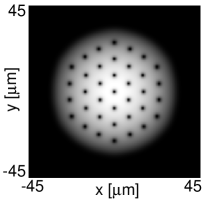
(b)
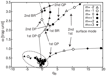
(c)

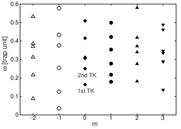
Figure 1: (a) Density profile of the condensate with 37 vortices at $\Omega=0.7\omega_{r}$. (b) Collective excitations up to $\omega=3.5\omega_{r}$. (c) Lowest excitations marked by a dotted line as functions of $q_{\theta}$ are displayed as functions of the symmetry index $m$. Here, TK, BR, DP, and QP denote the Tkachenko, breathing, dipole, and quadrupole modes, respectively.

The low-energy excitations are illustrated in Fig. 1. Here, the equilibrium states are found numerically via imaginary time propagation of Eq. (1); $t\rightarrow\tau=-it$. The initial vortex configuration is taken as a regular array with sixfold symmetry. The resulting configuration at $\Omega=0.7\omega_{r}$ is formed by 37 vortices, displayed in Fig. 1(a). In Fig. 1(b), the excitation energies up to $\omega=3.5\omega_{r}$ are shown as functions of the average angular momentum $q_{\theta}$. Each collective mode is classified by a symmetry index, $m$, obtained from the above function, $F^{(u)}_{\bf q}(m)$, which characterizes the oscillation pattern. For example, the breathing (BR), dipole (DP), and quadrupole (QP) modes have $m=0$, $\pm 1$, $\pm 2$, respectively. The branch extending from the origin towards higher $q_{\theta}$-values consists of surface modes which are spaced periodically with $m$ (mod 6), where the outer condensate surface oscillates, the vortex cores being almost stationary at their equilibrium positions. The other branch situated at higher energies and starting at $\omega=2\omega_{r}$ represents another class of surface modes characterized by a node along the radial direction. The energy spectra for the low-lying modes are depicted in Fig. 1(c) as functions of the symmetry index $m$. These low-lying eigenstates are the lattice-oscillation modes coupled with the condensate motion and lead to the distortion of both the lattice and the condensate surface towards an $m$-fold symmetric shape. In addition to the lowest and second-lowest TK with $m=0$, embedded among the other modes, we found a parallel-precession mode with $m=-1$ and having the lowest energy where all the vortices precess in phase. For increasing energy, the modes for each $m$ feature nodes along $r$ and/or $\theta$. The TK mode (with $m=0$) is selectively excited by the Gaussian laser beam with $0$-fold symmetry in the experiment coddington . Likewise, a mode with $m=\pm\ell$ may be excited by a disturbance (e.g., magnetic) with $\ell$-fold symmetry memo .

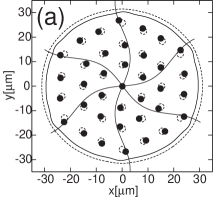
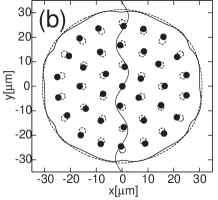
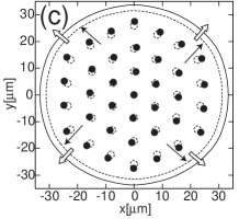
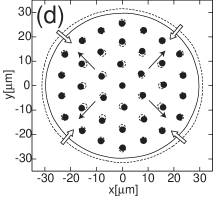
Figure 2: Oscillation patterns for the (a) lowest TK, (b) second TK, (c) lowest BR, and (d) second BR modes are indicated by the filled circles and solid lines. Empty circles and dotted lines correspond to the equilibrium state, $\phi_{g}$.

Figure 2 describes the oscillation patterns for selected collective modes obtained from a linear fluctuation $\delta\psi({\bf r},t)$: The lowest TK mode $\omega_{1,0}$ is shown in Fig. 2(a) where the empty (filled) circles indicate the equilibrium (quarter-period) positions of the vortex cores. The line is a fitted sinusoidal modulation wave (for clarity, the amplitude is magnified by a factor of $30$). It is observed that the modulation displays a node at $r_{\rm node}\simeq 0.64R_{\rm TF}$, which is in fair agreement with the JILA data of $r_{\rm node}=0.665R_{\rm TF}$. The second TK mode $\omega_{2,0}$ is shown in Fig. 2(b). It is seen that in contrast to the first TK mode whose core modulation is almost purely transversal, the second TK contains a longitudinal component, in addition to the transverse one. Thus, the core executes elliptic motion around its equilibrium position. This behavior coincides with the general trend for the ellipticity of a TK mode, namely the expression for the amplitude ratio of the longitudinal and transverse components $\delta_{\rm L}/\delta_{\rm T}\propto 1/\sqrt{\Omega}k_{\rm TK}$, where $k_{\rm TK}$ is the wavelength of the TK mode donnelly . Therefore, the second TK with a shorter $k_{\rm TK}$ exhibits more pronounced longitudinal motion. We also point out that via encountering the condensate radius in Figs. 2(a) and 2(b), the TK modes tend to accompany the condensate motion. We also observe that the ratio of the energies for these TK modes is $\omega_{2,0}/\omega_{1,0}=1.56$ at $\Omega=0.7\omega_{r}$, which compares favorably with the experimental data of $1.8\pm 0.2$ at $\Omega=0.95\omega_{r}$ coddington and with the value 1.63 obtained by Anglin and Crescimanno anglin , who assert that it would be independent of $\Omega$.

As typical vortex-lattice oscillations apart from the TK, we now consider two contrasting compressional modes which belong to the totally symmetric ($m=0$) “breathing” branch. Figures 2(c) and 2(d) depict the oscillation patterns for the lowest (1BR) and the second-lowest (2BR) breathing modes in Fig. 1(b). The former (latter) BR mode executes mutual in-phase (out-of-phase) motion between the cores and the condensate surface, as indicated with the two parallel (opposite) arrows in the figure. The inner (outer) arrow denotes the motion of the cores (condensates). Therefore, the former belongs to the common longitudinal mode and the latter to the differential longitudinal mode. It should be pointed out that the inner core motion in Figs. 2(c) and 2(d) is predominantly transversal; consequently, even in the nominally longitudinal BR mode all the vortex motion is not necessarily purely longitudinal. This may be related to the ‘$s$-bending’ coddington of the third observed mode.

Having obtained the complete spectrum of the low-lying excitations, let us now proceed to extend the analysis into nonlinear dynamics with real-time evolution simulated with the TDGP Eq. (1). Since Coddington et al. excite the TK mode by shining resonant laser light in the center of the BEC to produce an inward flow, we introduce a Gaussian potential $V({\bf r})=-\hbar\omega_{r}e^{-r^{2}/(R_{\rm TF}/2)^{2}}$ localized in the center of the trap for a certain period and follow the time evolution according to Eq. (1).

We illustrate the resulting oscillation patterns and their Fourier analyses in Fig. 3. At $\Omega=0.7\omega_{r}$, the 37 vortices shown in Fig. 1(a) form a concentric regular lattice around the central vortex, consisting of three circles, $j=1,2,3$. We analyze the transverse vortex motion ${\bf r}_{j,n}(t)=(x_{j,n}(t),y_{j,n}(t))$ in terms of the averaged angle $\theta_{j}(t)=\frac{1}{6}\sum^{5}_{n=0}[\arctan{(y_{j,n}(t)/x_{j,n}(t))}-\arctan{(y_{j,n}(0)/x_{j,n}(0))}]$ where $n$ denotes the vortices aligned along the line and extending the angle $n\pi/3$ from the vertical, see Fig. 1(a). It is apparent in Fig. 3(a) where we plot the time dependence of the vortex motion for each circle, $j=1,2,3$, that (i) there exist several superposed oscillations. (ii) The outermost vortices ($j=3$) are in opposite phase with the inner vortices ($j=1,2$). This result coincides with the above calculations based on the BdG equations. In fact, the nodal positions obtained from both calculations agree quite well.

(a)
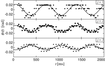
(b)

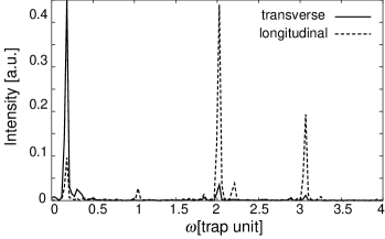
Figure 3: (a) Transverse oscillations of vortices on three concentric circles, $j=1,2,3$, from the trap center. (b) Fourier analyses of these oscillation patterns, $\theta_{j}(t)$, and the longitudinal vortex motion, $r_{j}(t)$.

In Fig. 3(b), the Fourier analyses of these transverse oscillations, $\theta_{j}(t)$, and the longitudinal motions, $r_{j}(t)=\frac{1}{6}\sum^{5}_{n=0}|{\bf r}_{j,n}(t)|$, are depicted. It is seen that the sharp peak at $\omega=0.16\omega_{r}$ precisely coincides with the first TK mode $\omega_{1,0}$ identified above, see Fig. 1(c). The second peak at $\omega=2.0\omega_{r}$ corresponds to the 1BR mode, belonging to the common longitudinal modes. The third peak at $\omega\sim 3.1\omega_{r}$ may be identified as the 2BR mode, see Figs. 1(b) and 2(d), and as a differential longitudinal mode. These three collective modes closely match the observed characteristics. In particular, the third mode which was tentatively assigned by Cozzini et al. and Choi et al. stringari , independently, as a higher-order hydrodynamic mode, is now identified above. It should be noted that the resonances of these three modes for a Gaussian potential have been numerically reproduced over a wide range of rotation rates $\Omega=0.7\sim 0.92$, corresponding to $37\sim 121$ vortices.

In Fig. 4, we plot the first TK energy $\omega_{1,0}$ as a function of $\Omega/\omega_{r}$ together with the experimental data coddington and a hydrodynamic prediction by Anglin and Crescimanno anglin . There prevails close quantitative overall agreement between our results and the experimental data. We emphasize that our calculations contain no adjustable parameters and also that our computations within the BdG and TDGP approaches agree within numerical accuracy $\sim 10^{-3}\omega_{r}$ below $\Omega\leq 0.8\omega_{r}$. Calculations for larger rotation rates, where BdG cannot be feasible from a numerical point of view, are done with TDGP, which enables us to extrapolate the BdG results to larger rotation rates. The inset in Fig. 4 describes the $\Omega$ dependence of the 1BR and 2BR modes. It is known that the former is consistent with an earlier prediction by Pitaevskii and Rosch pitaevskii , who point out that the 2D BR mode features the universal eigenfrequency $\omega=2.0\omega_{r}$. Our result reproduces this result and further explains the observation mentioned above that the second peak in Fig. 3(b) is indeed the 1BR mode. As for the third peak in Fig. 3(b), previously identified as the 2BR mode, it is reckoned from this inset that the observed value $18.5\pm 0.3$Hz ($\simeq 2.2\omega_{r}$) appears accountable, judging from the overall $\Omega$ dependence towards $\Omega_{c}$.

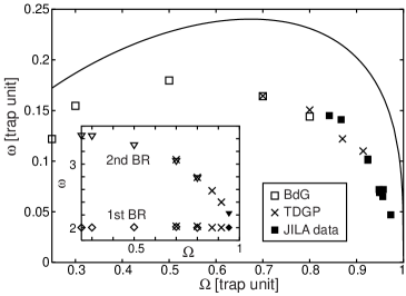
Figure 4: Frequencies of three modes obtained from the BdG and TDGP approaches are compared with the JILA data (filled squares, diamonds, and triangles) as functions of $\Omega$. In the main panel the TK (open squares), in the inset both the first BR (open diamonds) and the second BR (open triangles). The solid line represents the dispersion relation in Ref. anglin .

In summary, we have discussed the complete low-energy excitation spectrum in a vortex lattice by solving the BdG equations. The $m=0$ subset of these solutions includes the transverse shear, common longitudinal, and differential longitudinal modes. We have also succeeded in simulating the actual experimental results, identifying a new pair of modes.

The authors thank V. Schweikhard, I. Coddington, and M. Ichioka for useful conversations and communications. KM is grateful to G. Baym, J. R. Anglin, S. Stringari, and A. L. Fetter for enthusiastic discussions on the Tkachenko mode at the Aspen Center for Physics.

During the preparation of this manuscript, we learned about two closely related preprints baksmaty and simula . The former (latter) presents BdG (TDGP) treatments of the TK mode.

References

- (1) R. J. Donnelly, Quantized Vortices in Helium II (Cambridge University Press, Cambridge, 1991).
- (2) M. R. Matthews et al., Phys. Rev. Lett. 83, 2498 (1999).
- (3) A. E. Leanhardt et al., Phys. Rev. Lett. 89, 190403 (2002).
- (4) K. W. Madison et al., Phys. Rev. Lett. 84, 806 (2000).
- (5) J. E. Williams and M. J. Holland, Nature (London) 401, 568 (1999).
- (6) M. Nakahara et al., Physica B 284-288, 17 (2000).
- (7) V. K. Tkachenko, Sov. Phys. JETP 29, 245 (1969).
- (8) G. Baym, Phys. Rev. B 51, 11697 (1995).
- (9) M. R. Williams and A. L. Fetter, Phys. Rev. B 16, 4846 (1977).
- (10) L. J. Campbell, Phys. Rev. A 24, 514 (1981).
- (11) E. B. Sonin, Rev. Mod. Phys. 59, 87 (1987).
- (12) C. D. Andereck and W. I. Glaberson, J. Low Temp. Phys. 48, 257 (1982).
- (13) I. Coddington et al., Phys. Rev. Lett. 91, 100402 (2003).
- (14) This has been confirmed by our numerical simulations of the TDGP equations for .
- (15) J. R. Anglin and M. Crescimanno, cond-mat/0210063.
- (16) G. Baym, Phys. Rev. Lett. 91, 110402 (2003).
- (17) M. Cozzini and S. Stringari, Phys. Rev. A 67, 041602 (2003); S. Choi et al., Phys. Rev. A 68, 031605 (2003).
- (18) A. J. Leggett, Rev. Mod. Phys. 73, 307 (2001).
- (19) T. Isoshima et al., Phys. Rev. A 68, 033611 (2003).
- (20) L. P. Pitaevskii and A. Rosch, Phys. Rev. A 55, R853 (1997).
- (21) L. O. Baksmaty et al., cond-mat/0307368.
- (22) T. P. Simula et al., cond-mat/0307130.