Ferromagnetism in the Strong Hybridization Regime of the Periodic Anderson Model

Abstract

We determine exactly the ground state of the one-dimensional periodic Anderson model (PAM) in the strong hybridization regime. In this regime, the low energy sector of the PAM maps into an effective Hamiltonian that has a ferromagnetic ground state for any electron density between half and three quarters filling. This rigorous result proves the existence of a new magnetic state that was excluded in the previous analysis of the mixed valence systems.

Rigorous results, numerical and analytic, have greatly aided the study of strongly correlated electrons systems. Unfortunately, few such results exist. The numerical renormalization group and Bethe ansatz solutions of the single impurity Anderson and Kondo models are perhaps the best examples of a solid numerical approach and exact solution of simple models that changed and solidified the thinking in what was a highly controversial and puzzling problem area. Another important result was the rigorous connection between the two models established by Schrieffer and Wolff [1]. Their work showed that the low lying energy spectrum of the Anderson model in the strong coupling and weak hybridization limit ($U/t\gg 1$ and $V\ll|E_{F}-\epsilon_{f}|$) can be mapped into the Kondo model in the weak coupling regime ($J/t\ll 1$).

For dense systems, the natural extensions of the impurity models are the periodic Anderson (PAM) and Kondo lattice (KLM) models. For these, numerical renormalization group and Bethe Ansatz solutions are lacking even in one-dimension. In addition, very few rigorous results are available for the PAM [2, 3]. What remains true however is the connection between the strong and weak coupling limits via a natural extension of the Schrieffer-Wolff transformation.

There are two basic questions one can ask about these lattice models: what is their relevance to real materials and in what other parameter regimes might their physics be connected? In several well known papers, Doniach [4], at least implicitly, made several assumptions about the answers to both questions and proposed the now standard picture of the magnetic properties of f-electron materials that portrays a competition between the RKKY magnetic interaction which is obtained from a fourth order expansion in the hybridization and the Kondo exchange.

The reasoning behind this intuitively appealing picture is something like the following: From the Schrieffer-Wolff perturbation theory, the Kondo exchange coupling is related to the parameters in the PAM via $J\approx|V|^{2}/|E_{F}-\epsilon_{f}|$. In the PAM, a mixed valence regime corresponds to positioning the f-electron orbitals in the conduction band near the Fermi energy, i.e., $|E_{F}-\epsilon_{f}|\approx 0$. In this regime, the Schrieffer-Wolff result suggests the Kondo exchange is strong and thus can lead to a complete compensation of the f-moments by one or more of the conduction band electrons. Implied in this line of reasoning there are two important assumptions [4]: I) The strong coupling limit of the KLM is connected to the mixed valence regime (for weak hybridzation $|V|\ll|t|$) of the PAM, and II) the number of conduction electrons per $f$-magnetic moment is larger than one. Regarding the first assumption, we note that this connection is not established by the Schrieffer-Wolff transformation because when $|E_{F}-\epsilon_{f}|\approx 0$, the transformation is no longer valid.

We also note recent numerical studies [5, 6] of the weak hybridzation, strongly coupled PAM that find over a wide range of parameters ferromagnetic states which are not a result of the RKKY interaction and non-magnetic states which are not a consequence of a Kondo-like compensation of the f-moments by the conduction band electrons [7]. Additionally, there are mixed valence materials which exhibit a co-existence of ferromagnetism and a strong Kondo-like behavior (e.g., CeSi_x [8], CeGe₂ [9], Ce(Rh_1-xRu_x)₃B₂ [10], CeSi_1.76Cu_0.24 [11], Ce₃Bi₄, and CeNi_0.8Pt_0.2[12]). Because the RKKY interaction is considerably weaker than the Kondo exchange, these experimental results suggest that a ferromagnetic mechanism other than RKKY, at least sometimes, dominates in mixed valence materials.

In this paper we note that a strong hybrization, $|V|\gg|t|$, can lead to mixed valence state and a one-on-one compensation of an f-moment by a conduction electron. Then, for the strong couping limit of the one-dimensional KLM we rigorously establish that the ground state is connected to the strong hybridzation, strong coupling limit of the PAM. We thus show that Doniach’s first assumption is valid if the hybridization is strong, although its validity remains questionable for the more relevant regime $|V|\ll|t|$ (weak hiybridization). In the strong hybridization limit we rigorously show that there is ferromagnetic ordering instead of a nonmagnetic Kondo state. The difference between our result and Doniach’s can be attributed to the violation of his second assumption which indeed is not valid for a lattice system (one $f$-orbital per unit cell) since the number of conduction electrons (with net magnetic moment) per $f$ spin cannot be larger than one (it is equal to one only at half-filling).

The Hamiltonian for the one dimensional PAM is:

$$H = -t\sum^{L-1}_{{\bf i}=1,\sigma}(d_{{\bf i}\sigma}^{\dagger}d_{{\bf i}+1\sigma}+d_{{\bf i}+1\sigma}^{\dagger}d_{{\bf i}\sigma})+\epsilon_{f}\sum^{L}_{{\bf i}=1,\sigma}n_{{\bf i}\sigma}^{f}$$ (1)

$$- V\sum^{L}_{{\bf i}=1,\sigma}(d_{{\bf i}\sigma}^{\dagger}f_{{\bf i}\sigma}+f_{{\bf i}\sigma}^{\dagger}d_{{\bf i}\sigma})+\frac{U}{2}\sum^{L}_{{\bf i}=1,\sigma}n_{{\bf i}\sigma}^{f}n_{{\bf i}\bar{\sigma}}^{f}\ ,$$ (2)

where $d_{{\bf i}\sigma}^{\dagger}$ and $f_{{\bf r}\sigma}^{\dagger}$ create an electron with spin $\sigma$ in the $d$ and $f$ orbitals of the lattice site ${\bf i}$ and $n^{f}_{{\bf i}\sigma}=f^{\dagger}_{{\bf i}\sigma}f^{\;}_{{\bf i}\sigma}$.

We will show that for infinite $U$, $|t|\ll|V|$, and $|\epsilon_{f}|\lesssim|V|$ (asymmetric regime), the low energy sector of the PAM can be mapped into an infinite $U$ Hubbard model which includes correlated next-nearest neighbor hoppings and nearest-neighbor repulsions. To this end we first need to solve the atomic (one site) limit of the PAM [13] for all the possible fillings (0 to 3 particles per site because $U$ is infinite).

There are two possible eigenstates for one particle on one site ${\bf i}$. These eigenstates are created by the following operators:

$$\alpha_{{\bf i}\sigma}^{\dagger}=uf_{{\bf k}\sigma}^{\dagger}+vd_{{\bf i}\sigma}^{\dagger},\;\;\;\beta_{{\bf i}\sigma}^{\dagger}=-vf_{{\bf i}\sigma}^{\dagger}+ud_{{\bf i}\sigma}^{\dagger},$$ (3)

with

$$u=\frac{E_{1}^{+}-\epsilon_{f}}{\sqrt{(E_{1}^{+}-\epsilon_{f})^{2}+V^{2}}},\;\;v=\frac{V}{\sqrt{(E_{1}^{+}-\epsilon_{f})^{2}+V^{2}}}.\\$$ (4)

The operator $\alpha_{{\bf i}\sigma}^{\dagger}$ creates a particle in the bonding state with energy $E_{1}^{-}=\frac{\epsilon_{f}}{2}-\sqrt{\frac{\epsilon_{f}^{2}}{4}+V^{2}}$, while $\beta_{{\bf i}\sigma}^{\dagger}$ creates a particle in the anti-bonding state with energy $E_{1}^{+}=\frac{\epsilon_{f}}{2}+\sqrt{\frac{\epsilon_{f}^{2}}{4}+V^{2}}$ (see Fig. 1).

For two particles on one site, there are two singlets ($U=\infty$), and three triplet eigenstates (see Fig. 1). The ground and the highest energy states are the bonding and the anti-bonding singlets respectively:

$$|\phi^{-}\rangle = \frac{a}{\sqrt{2}}(f^{\dagger}_{{\bf i}\uparrow}d^{\dagger}_{{\bf i}\downarrow}-f^{\dagger}_{{\bf i}\downarrow}d^{\dagger}_{{\bf i}\uparrow})+b\;d^{\dagger}_{{\bf i}\uparrow}d^{\dagger}_{{\bf i}\downarrow},$$ (5)

$$|\phi^{+}\rangle = -\frac{b}{\sqrt{2}}(f^{\dagger}_{{\bf i}\uparrow}d^{\dagger}_{{\bf i}\downarrow}-f^{\dagger}_{{\bf i}\downarrow}d^{\dagger}_{{\bf i}\uparrow})+a\;d^{\dagger}_{{\bf i}\uparrow}d^{\dagger}_{{\bf i}\downarrow}.$$ (6)

with

$$a=\frac{E_{2}^{+}-\epsilon_{f}}{\sqrt{(E_{2}^{+}-\epsilon_{f})^{2}+2V^{2}}},\;\;b=\frac{\sqrt{2}V}{\sqrt{(E_{2}^{+}-\epsilon_{f})^{2}+2V^{2}}},\\$$ (7)

The energies of the bonding and the anti-bonding singlets are: $E^{\pm}_{2}=\frac{\epsilon_{f}}{2}\pm\sqrt{\frac{\epsilon_{f}^{2}}{4}+2V^{2}}$. The triplet states:

$$|\phi^{T}_{1}\rangle=f^{\dagger}_{{\bf i}\uparrow}d^{\dagger}_{{\bf i}\uparrow},\;\;\;\;\;|\phi^{T}_{-1}\rangle=f^{\dagger}_{{\bf i}\downarrow}d^{\dagger}_{{\bf i}\downarrow}$$ (8)

$$|\phi^{T}_{0}\rangle=\frac{1}{\sqrt{2}}(f^{\dagger}_{{\bf i}\uparrow}d^{\dagger}_{{\bf i}\downarrow}+f^{\dagger}_{{\bf i}\downarrow}d^{\dagger}_{{\bf i}\uparrow})$$ (9)

have energy $E^{T}_{2}=\epsilon_{f}$.

For three particles on one site, there are two possible states due to the two possible orientations of the $f$ spin: $f^{\dagger}_{{\bf i}\sigma}d^{\dagger}_{{\bf i}\uparrow}d^{\dagger}_{{\bf i}\downarrow}|0\rangle$. The energy of both states is $E_{3}=\epsilon_{f}$.

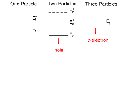
FIG. 1.: Energy levels for the atomic solution of the PAM for infinite $U$. The full lines correspond to the lowest energy levels that generate the reduced subspace of $H_{eff}$.

We will consider the range of concentrations: $\frac{1}{2}\leq n\leq\frac{3}{4}$, where $n=N_{e}/4L$ and $N_{e}$ is the total number of electrons. In this way, the concentration ranges from two to three particles per site. For $t=0$, the ground state of $H$ is massively degenerate, and the corresponding subspace is generated by states containing $L(3-4n)$ local bonding singlets $|\phi^{-}\rangle$ (doubly occupied sites) and $4L(n-\frac{1}{2})$ sites occupied by three particles. Therefore, the effective Hamiltonian which is obtained when $t$ is included perturbatively has a local dimension equal to 3 because each site can be occupied by a bonding singlet (hole) or by three particles state with two possible spin orientations (S=1/2 particle). The huge degeneracy of the ground state is then associated with both the spin and the charge degrees of freedom. We will see below that while the degeneracy associated with the charge degrees of freedom is lifted to first order in $t$, the spin degeneracy is lifted at second order.

To derive an effective Hamiltonian, we first need to identify the possible virtual processes. There are two different types of virtual (excited) states which are obtained by applying the hopping term to the ground state subspace of $H(t=0)$ (see Fig. 2): a) those in which two local nearest neighbor bonding singlets ($2+2$) are excited to local states having one and three particles ($1+3$) and b) those in which a local bonding singlet and a three particle state, which are nearest neighbors, are permuted and excited to the other possible local states (anti-bonding singlet or triplet). In any of these virtual processes, $t$ is much smaller than the energy difference between the virtual and the ground state because $|t|\ll|V|$ and $|\epsilon_{f}|\lesssim|V|$.

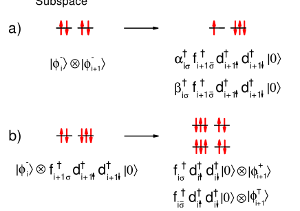
FIG. 2.: Virtual states which are obtained from the application of the hopping term $t$ to the lowest energy subspace of $H(t=0)$.

Introducing the creation and annihilation operators:

$$c^{\dagger}_{{\bf i}\sigma} = (1-n^{f}_{{\bf i}{\bar{\sigma}}})f^{\dagger}_{{\bf i}\sigma}d^{\dagger}_{{\bf i}\uparrow}d^{\dagger}_{{\bf i}\downarrow},$$ (10)

$$c^{\;}_{{\bf i}\sigma} = d^{\;}_{{\bf i}\downarrow}d^{\;}_{{\bf i}\uparrow}f^{\;}_{{\bf i}\sigma}(1-n^{f}_{{\bf i}{\bar{\sigma}}}),$$ (11)

and mapping the bonding singlet, $|\phi^{-}\rangle$, into the empty state or hole, we can write the effective Hamiltonian up to second order in $t$:

$$H_{eff} = -{\tilde{t}}\sum_{{\bf i},\sigma}(c^{\dagger}_{{\bf i}+1\sigma}c^{\;}_{i\sigma}+H.c.)+e_{0}\sum_{{\bf i}}(1-n_{\bf i})$$ (12)

$$+ t^{\prime}_{1}\sum_{{\bf i},\sigma}(c^{\dagger}_{i+1\sigma}n_{i}c^{\;}_{i-1\sigma}+H.c.)$$ (13)

$$+ t^{\prime}_{2}\sum_{{\bf i},\sigma,\sigma^{\prime}}(c^{\dagger}_{i+1\sigma^{\prime}}c^{\dagger}_{i\sigma}c^{\;}_{i\sigma^{\prime}}c^{\;}_{i-1\sigma}+H.c.)$$ (14)

$$+ t^{\prime}_{3}\sum_{{\bf i},\sigma}(c^{\dagger}_{i+1\sigma}(1-n_{\bf i})c^{\;}_{i-1\sigma}+H.c.)$$ (15)

$$+ g\sum_{{\bf i},\sigma}(1-n_{\bf i+1})(1-n_{\bf i})+\epsilon_{f}L$$ (16)

with

$${\tilde{t}} = \frac{ta^{2}}{2},\;\;\;\;\;\;t^{\prime}_{1}=\frac{t^{2}a^{2}}{2(E^{T}_{2}-E^{-}_{2})},\;\;\;\;\;\;$$ (17)

$$t^{\prime}_{2} = \frac{t^{2}a^{2}}{4}\Biggl{[}\frac{b^{2}}{E^{+}_{2}-E^{-}_{2}}-\frac{1}{E^{T}_{2}-E^{-}_{2}}\Biggr{]},$$ (18)

$$t^{\prime}_{3} = \frac{t{\tilde{t}}}{2}\Biggl{[}\frac{(au+\sqrt{2}vb)^{2}}{\epsilon_{f}+E^{-}_{1}-2E^{-}_{2}}+\frac{(av-\sqrt{2}ub)^{2}}{\epsilon_{f}+E^{+}_{1}-2E^{-}_{2}}\Biggr{]}$$ (19)

$$e_{0} = E^{-}_{2}-\epsilon_{f}-2{\tilde{e}}_{0}\;\;\;\;\;\;g=2{\tilde{e}}_{0}-4t^{\prime}_{3}$$ (20)

$${\tilde{e}}_{0} = \frac{t{\tilde{t}}}{2}\Biggl{[}\frac{b^{2}}{E^{+}_{2}-E^{-}_{2}}+\frac{3}{E^{T}_{2}-E^{-}_{2}}\Biggr{]}$$ (21)

The half-filled PAM corresponds to the absence of $c$ electrons (vacuum) and $n=\frac{3}{4}$ corresponds to one $c$ electron per site.

If we only keep the first order terms of $H_{eff}$, the resulting Hamiltonian is an infinite $U$ Hubbard model. In this model, the charge and the spin degrees of freedom are decoupled and therefore the wave function is a product of a charge and a spin component. As a consequence, the infinite $U$ Hubbard Hamiltonian maps into a spinless model for each fixed spin configuration. Therefore, the complete spin degeneracy persists to first order in $t$ while the charge degeneracy is lifted.

The second order terms introduce next nearest neighbor correlated hoppings $t^{\prime}_{1}$, $t^{\prime}_{2}$, $t^{\prime}_{3}$ and a repulsion $g$ between nearest neighbors. The terms $t^{\prime}_{1}$ and $t^{\prime}_{2}$ describe hopping processes where the electron hops over another electron in the intermediate site with and without spin flip. The $t^{\prime}_{3}$ term describes the hopping over an empty site. Notice that $t^{\prime}_{1}$ is the only term which can change the spin ordering.

Using a second order expansion around the strong coupling limit (large $J/t$) of the Kondo lattice model (KLM), Sigrist et al [14] found an effective Hamiltonian for the KLM of the same form as (7). The present result is more general. For specific choices of PAM parameters, (7) reduces to their result (and hence the eigenvalue spectra of two Hamiltonians become identical). The main point is that the equivalence in forms establishes a formal connection between the strong hybridization (mixed valence) and strong coupling regime of the PAM, and the strong coupling limit of the KLM. Given this connection, we recognize that the bonding singlet, represented by a hole in $H_{eff}$, is a Kondo singlet $|\phi^{-}\rangle$ in a mixed valence regime. It is interesting to remark that the large $J/t$ limit of the KLM has instead been associated to the small $U$ limit (weak coupling) of the PAM [15].

Sigrist et al [14] also proved that to leading order in $t^{\prime}_{i}$ ($1\leq i\leq 3$), the ground state of $H_{eff}$ is ferromagnetic for any concentration of $c$ electrons. To this end, they noticed that $t^{\prime}_{1}$ is the only relevant term since it can change the spin configuration. The particular sign of $t^{\prime}_{1}$ allowed them to apply the Perron-Frobenius theorem and demonstrate the ferromagnetic character of the ground state. Following exactly the same procedure, we can prove that the spin degeneracy of the 1D PAM for $t=0$ and $|\epsilon_{f}|\lesssim|V|$ is lifted in a perturbative sense toward a ferromagnetic state for any concentration $\frac{1}{2}\leq n\leq\frac{3}{4}$ with a total spin per site $2(n-\frac{1}{2})$.

The microscopic mechanism for the stabilization of the FM ground state is similar to the one found by Nagaoka [16] in the Hubbard model for dimension larger than one. Even though $H_{eff}$ is a one dimensional model, there are two different ways to move one hole to a next-nearest neighbor site by hopping over one $c$-electron: either by two applications of ${\tilde{t}}$ or by one application of $t^{\prime}_{1}$. Only when the background is FM will both processes give rise to the same final state. If the sign of the final state is the same for both processes, the effective matrix element is reinforced (constructive interference) and kinetic energy of the hole is lowered. This is indeed what happens in $H_{eff}$ due to the positive sign of $t^{\prime}_{1}$. Therefore, the coherent propagation of the Kondo singlet (hole) is responsible for the polarization of the spins which are not quenched by the conduction electrons. Since this coherent propagation is only possible for dense systems where the $f$-orbitals form a lattice, the stabilization of the FM state is excluded from any analysis which only considers the dilute limit (few $f$-orbitals).

The same perturbative analysis used to prove the FM character of the ground state can also be used to show [14, 17] that the low energy spin excitations of $H_{eff}$ are described by a FM Heisenberg model with an effective exchange interaction: ${\bar{J}}=2\frac{t^{\prime}_{1}}{\pi}[\frac{2}{\pi\rho}sin^{2}(\pi\rho)-sin(2\pi\rho)]$, where $\rho$ is the density of $c$-electrons. This effective Heisenberg model operates in a truncated Hilbert space of $H_{eff}$ that only contains spin degrees of freedom. The separation between charge and spin degrees of freedom occurs because to leading order in $t^{\prime}_{i}$, the eigenstates are still factorisable into their orbital and spin components.

In summary, we proved that the PAM has a ferromagnetic ground state in the strong hybridization and strong coupling regime for concentrations between half and three quarters filling. This wide region of concentrations clearly indicates that the microscopic mechanism is not related to an RKKY interaction as is expected for a strong mixed valence regime. Instead, the stabilization of the FM ground state is due to the coherent propagation of the Kondo singlets in a FM background. The mechanism is similar to the one operating in the Nagaoka [16] solution of the infinite $U$ Hubbard model.

It is important to ask what can we expect in higher dimensions. In this case, the spin degeneracy of $H(t=0)$ is lifted to first order in $t$ because there is no separation between the charge and the spin degrees of freedom. It is well known that the ferromagnetic Nagaoka [16] state is stabilized when one electron is added to the half filled system. Different works [18, 19, 20] indicate that a partially polarized FM state is favored for a finite range of concentrations away from half filling. In addition, we have recently found numerical evidence of itinerant ferromagnetism in the PAM for the mixed valence regime and $|V|\lesssim|t|$ [5, 6].

The current situation clearly merits reasking what are the possible scenarios when a dense system is away from half-filling to evolve from the localized to the mixed valence regime. In the localized regime, the hybridization can be considered as a perturbation and the corresponding perturbation theory tells us that the magnetic properties are dominated by the RKKY interaction. When the system approaches the mixed valence regime, there are at least two different possibilities: a) A paramagnetic Fermi liquid, where the absence of magnetic ordering is just a consequence of the Pauli exclusion principle (only a small fraction of the $f$-moment is screened by the conduction electrons) [7]; and b) A partially polarized FM metal (see also [5, 6]) The existence of this second scenario as a possible solution of the PAM provides a natural explanation for a number of U (US, USe, UTe [21], URu_2-xM_xSi₂ with M = Re, Tc and Mn [22]) and Ce based (CeSi_x [8], CeGe₂ [9], Ce(Rh_1-xRu_x)₃B₂ [10], CeSi_1.76Cu_0.24 [11], Ce₃Bi₄, and CeNi_0.8Pt_0.2[12]) materials which exhibit the coexistence of ferromagnetism and Kondo behavior.

In addition, we have established a connection between the strong hyridization limit of the PAM and the strong coupling limit of the KLM which is valid in any dimension. This connection provides a physical meaning for the strong coupling regime of the KLM.

Acknowledgements. This work was sponsored by the US DOE. J. B. acknowledges the support Slovene Ministry of Education Science and Sports and FERLIN.

REFERENCES

- [1] J. R. Schrieffer and P. A. Wolff, Phys. Rev. 149, 4910 (1996).
- [2] K. Ueda, H. Tsunetsugu and M. Sigrist, Phys. Rev. Lett. 68, 1030 (1992).
- [3] T. Yanagisawa and Y. Shimoi, Int. Jour. of Mod. Phys. B 10, 3383 (1996).
- [4] S. Doniach, Physica 91B, 231 (1977); R. Jullien, J. N. Fields and S. Doniach, Phys. Rev. B 16, 4889 (1977).
- [5] C. D. Batista, J. Bonča and J. E. Gubernatis, Phys. Rev. Lett. 88, 187203 (2002).
- [6] C. D. Batista, J. Bonča, J. E. Gubernatis, preprint.
- [7] J. Bonča and J. E. Gubernatis, Phys. Rev. B 58, 6992 (1998).
- [8] H. Yashima, H. Mori and T. Satoh, Solid State Commun. 43, 193 (1982).
- [9] R. Lahiouel, R. M. Galera, J. Pierre, E. Siaud and A. P. Murani, J. Magn. Magn. Mat. 63 64, 98 (1987).
- [10] S. K. Malik, A. M. Umarji, G. K. Shenoy and P. A. Montano and M. E. Reeves, Phys. Rev. B 31, 4728 (1985).
- [11] P. Böni, G. Shirane, Y. Nakazawa, M. Ishikawa and S. Tomiyoshi, J. Phys. Soc. Jpn. 56, 3801 (1987).
- [12] G. Fillion, M. A. Frémy, D. Gignoux, J. C. Gomez Sal and B. Gorges, J. Magn. Magn. Mat. 63 64, 117 (1987).
- [13] R. Chan and M. Gulácsi, Phil. Mag. Lett. 81, 673 (2001).
- [14] M. Sigrist, H. Tsunetsugu, K. Ueda, and T. M. Rice, Phys. Rev. B 46, 13838 (1992).
- [15] H. Tsunetsugu, M. Sigrist and K. Ueda, Rev. Mod. Phys. 69, 809 (1997).
- [16] Y. Nagaoka, Phys. Rev. 147, 392 (1966).
- [17] M. Ogata and H. Shiba, Phys. Rev. B 41, 2326 (1990); Int. J. Mod. Phys. B 5, 31 (1991).
- [18] X. Y. Zhang, E. Abrahams and G. Kotliar, Phys. Rev. Lett. 66, 1236 (1991).
- [19] W. O. Putikka, M. U. Luchini and M. Ogata, Phys. Rev. Lett. 69, 2288 (1992).
- [20] S. Liang and H. Pang, Europhys. Lett. 32, 173 (1995).
- [21] P. Santini, R. Lémanski and P. Erdös, Advan. in Phys. 48, 537 (1999).
- [22] Y. Dalichaouch, M. B. Maple, R. P. Guertin, M. V. Kuric, M. S. Torikachvili and A. L. Giorgi, Physica B 163, 113 (1990).