Thermodynamic properties of ferromagnetic mixed-spin chain systems

Abstract

Using a combination of high-temperature series expansion, exact diagonalization and quantum Monte Carlo, we perform a complementary analysis of the thermodynamic properties of quasi-one-dimensional mixed-spin systems with alternating magnetic moments. In addition to explicit series expansions for small spin quantum numbers, we present an expansion that allows a direct evaluation of the series coefficients as a function of spin quantum numbers. Due to the presence of excitations of both acoustic and optical nature, the specific heat of a mixed-spin chain displays a double-peak-like structure, which is more pronounced for ferromagnetic than for antiferromagnetic intra-chain exchange. We link these results to an analytically solvable half-classical limit. Finally, we extend our series expansion to incorporate the single-ion anisotropies relevant for the molecular mixed-spin ferromagnetic chain material MnNi(NO₂)₄(ethylenediamine)₂, with alternating spins of magnitude 5/2 and 1. Including a weak inter-chain coupling, we show that the observed susceptibility allows for an excellent fit, and the extraction of microscopic exchange parameters.

I Introduction

Promoted by the synthesis of various one-dimensional (1D) bimetallic molecular magnets, the physics of quantum spin chains with mixed magnetic moments is of great interest. Typically, quasi-1D mixed-spin (MS) compounds display antiferromagnetic (AFM) intra-chain exchange Kahn95 ; Caneschi89 ; Nishizawa00 , which has stimulated theoretical investigations of AFM MS models using a variety of techniques such as spin-wave theory Pati97a ; Pati97b ; Brehmer97 ; Yamamoto98aa ; Yamamoto98a ; Yamamoto98b ; Yamamoto98c , variational methods Kolezhuk97 , the density-matrix renormalization group (DMRG)Pati97a ; Pati97b ; Yamamoto98b , and quantum Monte Carlo calculationsBrehmer97 ; Yamamoto98aa ; Yamamoto98a ; Yamamoto98b ; Yamamoto98c . Interestingly, since a unit cell of the MS chain comprises of two different magnetic moments, the spectrum will allow for excitation of ‘acoustic’ as well as ‘optical’ nature Yamamoto98aa ; Yamamoto98b . While not identified unambiguously in present day experiments, the character of these excitations should appear in thermodynamic and other observable properties as two independent energy scales. Nakanishi02

In addition, and apart from the preceding, what remains less well studied are MS chains with ferromagnetic (FM) intra-chain exchange, which arise in materials of recent interest such as MnNi(NO₂)₄(en)₂ with en = ethylenediamine Feyerherm01 . This compound is regarded as a quasi-1D MS material with spins $S=5/2$ and $s=1$ at the Mn and Ni ions, respectively. The susceptibility displays an easy-axis anisotropy. At temperatures below $T_{N}=2.45\textrm{K}$, a weak AFM inter-chain coupling induces AFM ordering. If this antiferromagnetic order is suppressed by a magnetic field of approximately 1.6T, the low-temperature specific heat shows a maximum at $T=6\textrm{K}$ and a shoulder at $T=1.5\textrm{K}$. These features could possibly reflect the two aforementioned characteristic energy scales, however for the case of an FM, rather than an AFM MS chain.

Motivated by this, it is the purpose of this paper to perform a complementary analysis of the thermodynamic properties of FM MS chains, using high-temperature series expansion (HTSE), exact diagonalization (ED), and quantum Monte Carlo (QMC). In particular, our HTSE will be derived for arbitrary alternating spins $S$ and $s$. This will allow not only for a direct comparison with experimental data, but also for a study of a gradual transit to the ‘half-classical’ limit $S\rightarrow\infty$ which is exactly solvable Dembiski75 ; Seiden83 ; Kahn92 . Finally, while our ED and QMC data will be obtained on systems of the smallest possible mixed-spin magnitude, i.e. $S=1$ and $s=1/2$, this is a case also included in the HTSE. In addition, for the sake of completeness and to compare with existing literature, we will also include results for the AFM case.

In this paper, we focus on a chain with two kinds of spin species, i.e. $S$ and $s$, arranged alternatingly and coupled by a nearest-neighbor Heisenberg exchange. Namely, the Hamiltonian reads

$$\mathcal{H}_{\textrm{int}}=-J\sum_{i=1}^{N}\left(\mathbf{S}_{i}\cdot\mathbf{s}_{i}+\mathbf{s}_{i}\cdot\mathbf{S}_{i+1}\right).$$ (1)

The subscript $i=1\ldots N$ refers to the unit cells, and we always use periodic boundary conditions.

In section II, our HTSE approach is detailed. In section III, we turn to a comparison with QMC and ED and the results of the ‘half-classical’ limit. In section IV, we discuss the result of fitting the HTSE to susceptibility data obtained for MnNi(NO₂)₄(en)₂. Conclusions are presented in section V.

II High-temperature series expansion

The HTSE is an expansion in powers of $\beta J$, where $\beta$ is the inverse temperature. Here we use the linked-cluster expansion of Ref. Domb3, . In this method, the series coefficients for the thermodynamic limit are obtained exactly from those calculated on finite-size clusters. In general, this includes the subtraction of contributions from a large number of so-called subclusters. In one dimension, however, significant simplifications occur due to cancellation Baker64 ; Fukushima03 . This is true also for the MS chain systems. That is, in the absence of a magnetic field, the free energy $F$ in the thermodynamic limit is represented by

$$F/N = F_{\ell}(S,s)+F_{\ell}(s,S)$$ (2)

$$-F_{\ell-1}(S,s)-F_{\ell-1}(s,S)+O[(\beta J)^{2\ell}],$$

where $F_{\ell}(S,s)$ is the free energy of the $\ell$-site open-chain system described by

$$\mathcal{H}_{\ell} = -J\sum_{i=1}^{(\ell-1)/2}\left(\mathbf{S}_{i}\cdot\mathbf{s}_{i}+\mathbf{s}_{i}\cdot\mathbf{S}_{i+1}\right)\;(\ell:\textrm{odd})$$ (3)

$$= \mathcal{H}_{\ell-1}-J\mathbf{S}_{\frac{\ell}{2}}\cdot\mathbf{s}_{\frac{\ell}{2}}\;\;(\ell:\textrm{even}),$$

and $F_{\ell}(s,S)$ is obtained by exchanging $S$ and $s$ in $F_{\ell}(S,s)$. Then, a calculation of $\textrm{Tr}[(\mathcal{H}_{\ell})^{n}]$ is needed on a finite system, i.e.,

$$\textrm{Tr}\mathcal{H}_{\ell}^{n}=\sum_{\{m_{i}\}}\langle m_{1}\ldots m_{\ell}|\mathcal{H}_{\ell}^{n}|m_{1}\ldots m_{\ell}\rangle,$$ (4)

where $m_{i}$ represents the magnetic quantum numbers at site $i$. We apply $\mathcal{H}_{\ell}$ order by order on the ket $|m_{1}\ldots m_{\ell}\rangle$. This operation yields linear combinations of kets with coefficients which are functions of $\{m_{i}\}$. To evaluate $\textrm{Tr}\mathcal{H}_{\ell}^{2n}$, products of kets of type $\mathcal{H}_{\ell}^{n}|m_{1}\ldots m_{\ell}\rangle$ are needed at most, while in the case of Tr$\mathcal{H}_{\ell}^{2n+1}$, one can use that $\mathcal{H}_{\ell}^{2n+1}=\mathcal{H}_{\ell}^{n}\mathcal{H}_{\ell}^{n+1}$. In order to evaluate this trace, we use two different algorithms.

Method (i) is based on a direct matrix multiplication for fixed $S$ and $s$. A linear combination of kets with coefficients is regarded as a sparse vector. It is stored as a compressed array of non-zero elements and another array of their pointers to the kets. These pointers are stored in the ascending order so that one can find a needed element using binary search in the array. All the operations are performed using integers, and thus there is no loss of precision.

Method (ii) is designed for arbitrary spins, which is based on an analytic approach to the matrix elements in Eq. (4). It has an advantage for large spins because the method (i) will fail for very large spins due to time and/or memory constraints. After symbolic operations, the summation of the form $\sum_{m=-s}^{s}m^{n}$ can be calculated analytically for arbitrary $n$. For example, when $n=2$, the sum is equal to $\frac{1}{3}s\,(s+1)(2s+1)$. As a result, the series coefficients are obtained as an expression valid for arbitrary $S$ and $s$. Naively it may seem that operators of type $s^{\pm}$ will causes square roots in the matrix elements of the Hamiltonian. However, such square roots are absent in the final result. In fact, the calculation can be carried out disregarding square roots as explained below. Introducing the simplified notation,

$$|\pm n_{1}\ldots\pm n_{\ell})\equiv(s_{1}^{\pm})^{n_{1}}\ldots(s_{\ell}^{\pm})^{n_{\ell}}|m_{1}\ldots m_{\ell}\rangle.$$ (5)

the initial state is represented by $|0\ldots 0)$. Spin operators act on these states as follows. Suppose $|\pm n)$ ($n$¿0) represents the state at site $i$ in the notation (5). Then,

$$s^{z}|\pm n) =(m\pm n)|\pm n),$$ (6)

$$s^{\pm}|\pm n) =|\pm n\pm 1),$$ (7)

and

$$s^{\mp}|\pm n) = s^{\mp}s^{\pm}|\pm n\mp 1)$$ (8)

$$= |\pm n\mp 1)\times$$

$$\;\left\{s(s+1)-(m+n\mp 1)(m+n)\right\}.$$

Note that the norm of $|n)$ is not unity, namely,

$$(\pm n|\pm n)=\prod_{n^{\prime}=1}^{n}\left\{s(s+1)-(m+n^{\prime}\mp 1)(m+n^{\prime})\right\}.$$ (9)

Besides the methods (i) and (ii), the contribution to the specific heat from the largest cluster is calculated separately. Namely, contributions from $\ell$-site chain to $O[(\beta J)^{2\ell-2}]$ and $O[(\beta J)^{2\ell-1}]$ have a simple form; with notation $x\equiv s(s+1)$ and $X\equiv S(S+1)$, for $\ell=2l$ it is proportional to 2$l$ $x^{l}X^{l}$ and for $\ell=2l+1$ to $x^{l}X^{l+1}+x^{l+1}X^{l}$. The prefactors of these terms can be determined by comparing with those of $s=S=1/2$ for any $\ell$ in Ref. Fukushima03, . The methods (i) and (ii) are used only for the rest of the contribution.

We have computed the specific heat for the model (1) with $s=1/2$ and $S=1$, up to 29th order using the method (i). Furthermore, for arbitrary $s$ and $S$, the series has been calculated up to 11th order using the method (ii) and standard symbolic packages Mathematica . By setting $S=s=1/2$, our model is reduced to the homogeneous spin-half Heisenberg chain, and our series agrees with that in the literatureBaker64 . Furthermore, we have also checked that the $S\rightarrow\infty$ limit of the series agrees with the Taylor series of the exact solutionDembiski75 which will be shown in the next section.

III large- and small-spin limits

In this section, we provide evidence for the presence of a double-peak-like structure in the specific heat of the FM MS chain. We begin by recalling the elementary excitations in an MS chain. The dispersion relation of the one-magnon excitations in the FM case reads

$$\omega(k)=J\left(S+s\pm\sqrt{S^{2}+s^{2}+2Ss\cos(k)}\right),$$ (10)

and is shown in Fig. 1 for the extreme quantum case, $s=1/2$ and $S=1$. Similar to the AFM caseYamamoto98aa ; Yamamoto98b , the spectrum consists of both an acoustic and an optical branch reflecting the presence of two different spins in a unit cell. These branches indicate two energy scales in the thermodynamics of the MS chains. The appearance of two one-magnon branches can be qualitatively understood as follows: At $k=\pi$, the excitations correspond to an alternating tilting of either the shorter or the longer spins as indicated by the arrows in Fig. 1. The magnitude of neighboring spins determines the energies of these modes, leading to a splitting of the branches for $S\neq s$. As $k$ is reduced away from $k=\pi$, the magnon eigenstates gradually loose these alternating tilting form, and near $k=0$ become similar in nature to those of uniform chains. The low-temperature specific heat as computed using linear spin-wave theory is expected to be exactTakahashi85 to leading order in $T$. Since $\omega(k)$ is proportional to $k^{2}$ at low energies, the specific heat is thus proportional to $T^{1/2}$ for $T\ll J$.

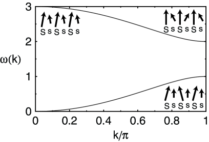
Figure 1: The spin-wave dispersion relation for the FM MS chain with $s=1/2$ and $S=1$. The spatial distance of two spins of the same species in neighboring unit cells is taken to be unity.

We can establish a connection between the high-temperature series for the specific heat and this low-temperature scaling using a suitable Padé analysis. In extrapolating the high-temperature series for the specific heat, information from the ground-state energy, the low-energy excitations, and the high-temperature entropy can be used as follows Bernu01 : The expansion variable is changed from $\beta$ to the internal energy per unit cell, $e=\langle\mathcal{H}_{\textrm{int}}\rangle/N$. Here, $e=0$ for $\beta=0$. The power series of $e(\beta)$ is thus inverted to obtain $\beta(e)$. Let $\mathcal{S}(e)$ denote the entropy per unit cell of the MS chain. From $\beta=\textrm{d}\mathcal{S}/\textrm{d}e$, one obtains

$$\mathcal{S}=\mathcal{S}_{T=\infty}+\int_{0}^{e}\beta(e^{\prime})\textrm{d}e^{\prime},$$ (11)

where $\mathcal{S}_{T=\infty}=\ln(2S+1)+\ln(2s+1)$. The low-temperature behavior of the specific heat, $C\propto T^{1/2}$, translates into $\mathcal{S}\propto(e-e_{0})^{1/3}$ at $e\sim e_{0}$ for the new series, where $e_{0}$ is the ground state energy per site. In Ref. Bernu01, , only the FM $e_{0}$ is used to extrapolate the specific heat of a HTSE for a FM model. Here, we also employ the AFM $e_{0}$, since this additional constraint from the other sign of $J$ does not drastically change the final result, but makes the extrapolation less sensitive to the used Padé approximant. We thus obtain the same extrapolation for both the FM and the AFM case. Namely, the AFM specific heat will be obtained using the substitutions $e\rightarrow-e$ and $\beta J\rightarrow-\beta J$ from the FM case. Then, if the Padé approximant in $e$ is applied to

$$\mathcal{S}^{3}\Big{(}\ln(2S+1)(2s+1)\Big{)}^{-3}\left(1-\frac{e}{e_{0}^{\rm FM}}\right)^{-1}\left(1+\frac{e}{e_{0}^{\rm AFM}}\right)^{-1},$$

the low-temperature behavior and the high-temperature entropy are correctly reproduced. For $s=1/2$ and $S=1$, we use the AFM ground-state energy $e_{0}^{\rm AFM}=-1.45408J$ from Ref. Pati97a, . The extrapolation is found to be rather insensitive to errors in $e_{0}^{\rm AFM}$. For example, an error $10^{-4}J$ in $e_{0}^{\rm AFM}$ affects the AFM specific heat only by $4\times 10^{-4}$ at $T=0.1J$, and even less at higher temperatures. In the following we denote by $P[m/n]$ the rational approximant function in $e$ resulting from a polynomial of order $m$ over a polynomial of order $n$.

In Fig. 2, a comparison is shown between different Padé approximants for the low-temperature specific heat for the $s=1/2$, $S=1$ case. We also include results from stochastic series expansion QMC simulations wessel for both the FM and the AFM case for chains of 100 sites. No deviations were found to the QMC data for 50 sites, and thus we regard these results to represent the thermodynamic limit. For the AFM case, the DMRG results from Ref. Yamamoto98b, are shown in Fig. 2a as well. In contrast to the AFM case, the HTSE result for the low-temperature specific heat for the FM case shows large oscillation upon increasing the order of the series. Comparison with the QMC data shows that the exact solution is located within the range of these oscillations. We take the arithmetic average of $P[12/11]$, $P[13/12]$, $P[14/13]$ and $P[15/14]$ as the final HTSE result, which in the temperature range $0.03J<T<0.45J$ has an error of order 5%.

The specific heat in a larger temperature regime is shown in Fig. 3. We find overall good agreement between the QMC and the HTSE data, both for the AFM and the FM case. In contrast to the homogeneous FM spin-1/2 chain, the FM MS chain displays at least two distinct structures in $C(T)$, namely a peak at $T\sim 0.54J$ and a shoulder at $T\sim 0.25J$. The HTSE result indicates the presence of an additional weak shoulder at $T\sim 0.1J$, which is however difficult to check for using QMC due to increasing statistical errors at that low temperatures.

The features in the intermediate temperature regime become more pronounced with increasing order of the series expansion, probably because the higher-order polynomials can reproduce the involved rapid changes more accurately.

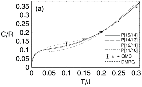
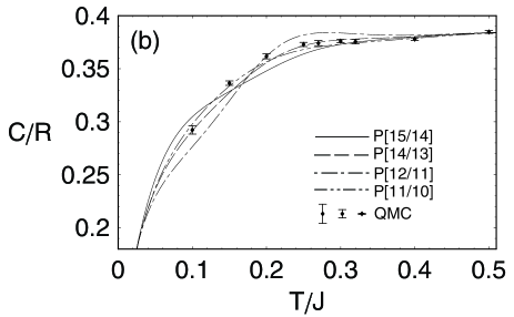
Figure 2: Low-temperature behavior of the specific heat per unit cell of the AFM (a) and FM (b) mixed-spin chain with $s=1/2$, $S=1$ using several different Padé approximants of the HTSE and from QMC. In (a), DMRG results from Ref. Yamamoto98b, are also shown. Here, $R$ is the gas constant.

We have included in Fig. 3 ED results for small finite chains for both the AFM and the FM case. The full spectrum has been calculated for finite chains with up to 7 unit-cells (14 sites). The ED result for 14 sites agrees with the QMC and the HTSE down to temperatures of $T\sim 0.5J$ for the FM case, and $T\sim 0.3J$ for the AFM case. Fig. 3 clearly shows that finite-size effects in the specific heat are significantly larger in the FM than in the AFM case. In the AFM case, the differences between the 12- and 14-site data are already rather small, with a weak shoulder at low temperature signaling the second energy scale in $C\left(T\right)$. For the FM case the ED data show a strong finite-size shift of the specific heat maximum, which gradually develops into the shoulder near $T\sim 0.25J$, which is found both from the HTSE and QMC.

This suggests that long-range collective modes dominate the thermodynamics up to higher temperatures for the FM than for the AFM case. To shed more light onto this difference, let us compare the elementary excitation spectra for the FM and the AFM case: (i) At low temperatures, the specific heat reflects the dispersion of the acoustic branch of excitations. In the long-wavelength limit, the dispersion in linear spin-wave theory reads

$$\omega(k)\sim\frac{Ss}{2|S\pm s|}k^{2},$$

where the plus (minus) sign represents the FM (AFMPati97a ; Brehmer97 ) case. Therefore, the slope of the acoustic branch in the AFM case is larger than in the FM case, making low-temperature shoulders more pronounced for FM MS chains. (ii) The gap between the acoustic and the optical mode in the FM case is larger than in the AFMYamamoto98aa ; Yamamoto98b case, so that the splitting of the structures in $C(T)$ is more evident in the former case. Apart from (i) and (ii), the elementary excitation spectra of the FM and the AFM case resemble each other, pointing towards additional effects from magnon interactions.

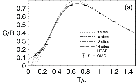
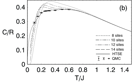
Figure 3: Specific heat per unit cell of the AFM (a) and FM (b) mixed-spin chain with $s=1/2$, $S=1$ as obtained from HTSE, QMC and full diagonalizations for small finite chains.

After analyzing the extreme quantum case with $s=1/2$ and $S=1$, we now discuss the specific heat of MS chains for larger values of $S$, keeping $s=1/2$ fixed. In particular, we want to connect to the exactly solvable Dembiski75 ‘half-classical’ limit, $S\rightarrow\infty$.

Fig. 4 shows the results from the 11th order HTSE for $s=1/2$ and various values of $S$. The temperature is normalized to $|\mathbf{S}|J\equiv J\sqrt{S(S+1)}$ in order to render the ’half-classical’ limit finite. In the limit $S\rightarrow\infty$ the specific heat of the chain with FM couplings is identical to that of the AFM chain, with a distinct peak at $T\sim 0.5\,|\mathbf{S}|J$. At $T=0$ the specific heat of the ‘half-classical’ model is finite. In the quantum case, however, the specific heat vanishes as $T\rightarrow 0$. Using the variable $S$ HTSE, we can link both limiting situations as follows: In the limit $S\rightarrow\infty$, the series coefficients of $(\beta SJ)^{n}$ with odd $n$ converge to zero. Let us compare the $(2n)$-th and $(2n+1)$-th order terms at finite $S$. The ratio of the latter to the former is of $O(t/S)$, where $t\equiv T/(SJ)$. Hence, if the limit $S\rightarrow\infty$ is taken with $t$ fixed, the latter becomes negligible compared to the former as $S\rightarrow\infty$. However, if $S$ is finite, the two terms are comparable for temperatures below $t\sim S^{-1}$. Therefore, even if $S$ is large, the specific heat deviates from the ’half-classical’ behavior below $t\sim S^{-1}$, and approaches zero as $t\rightarrow 0$. As a result, the specific heat will display a double-peak-like structure for large $S$ as well. Summarizing these results from the HTSE, there are two different ways of taking the large-$S$ and $T\rightarrow 0$ limit,

$$\lim_{T\rightarrow 0}\lim_{S\rightarrow\infty}C/R = 1,$$ (12)

$$\lim_{S\rightarrow\infty}\lim_{T\rightarrow 0}C/R = 0.$$ (13)

As seen from Fig. 4 the difference between the FM and the AFM cases are most pronounced in the extreme quantum limit $s=1/2$ and $S=1$, and in the low-temperature regime. The large- and small-spin limits exhibit similar structures, suggesting that the specific heat of MS chain systems in general show a double-peak-like or peak-shoulder structure, both for AFM and FM intra-chain exchange, and for any combination of spins. In the FM case this structure is more pronounced if $|S-s|$ is large, reflecting the size of the gap between the acoustic and the optical mode, similar to the AFM case.Nakanishi02

We note that the specific heat in the high-temperature limit of the AFM case is larger than in the FM case because of quantum effects. This is evident from the first two terms of the series for the specific heat, which we present in Appendix A. These two terms stem from two-site correlations only and dominate the high-temperature behavior. Since the total entropy difference between zero and infinite temperature is the same in both cases, the FM and AFM specific-heat curves therefore have to intersect at low temperatures.

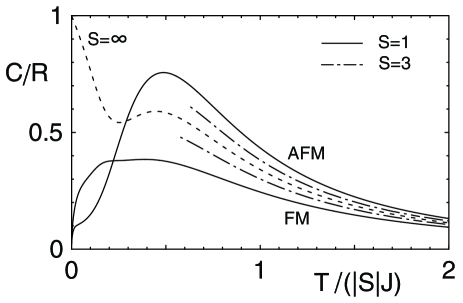
Figure 4: The HTSE results for the dependence on $S$ of the specific heat per unit cell with $s=1/2$ for antiferromagnetic (AFM) and ferromagnetic (FM) coupling, where $|\mathbf{S}|=\sqrt{S(S+1)}$. Here, $S=\infty$ is from Ref. Dembiski75, . Details are in the text.

IV fitting to experimental data

We now turn to a comparison to the susceptibility data observed on MnNi(NO₂)₄(en)₂. In this compound, the symmetry around Ni ions is nearly cubic with however a fairly large anisotropy at the Mn site to be expected Feyerherm01 . Hence, we take into account a single-site anisotropy only on one of the spins, i.e. $S$. The g-factors of the spins $S$ and $s$ are represented by $G$ and $g$, respectively. Therefore, the total Hamiltonian reads

$$\mathcal{H}=\mathcal{H}_{\textrm{int}}+\mathcal{H}_{\textrm{ani}}+\mathcal{H}_{\textrm{mag}},$$ (14)

where

$$\mathcal{H}_{\textrm{ani}} = D\sum_{i=1}^{N}\left(S_{i}^{z}\right)^{2},$$ (15)

$$\mathcal{H}_{\textrm{mag}} = -\mathbf{h}\cdot\sum_{i=1}^{N}(G\,\mathbf{S}_{i}+g\,\mathbf{s}_{i}).$$ (16)

Here, we derive the power series of $\chi$ in $\beta D$ as well as $\beta J$ up to $O(\beta^{7})$. When $D=0$ and $g=G$, the series coefficients coincide with those in the literatureWojtowicz67 ; Freeman72 assuming a misprintmisprint in Ref. Wojtowicz67, . Since the contribution $\mathcal{H}_{\textrm{mag}}$ is used to evaluate the susceptibility we will only consider the case of small Zeeman energies $\left|\mathbf{h}\right|=h\rightarrow 0$ in the following. The orientation of the magnetic field $\mathbf{h}$ will be chosen to be either $\mathbf{h}\|z$ or $\mathbf{h}\|x$. Most theoretical studies of MS systems are limited to the case of $D=0$ and $g=G$, in order to make use of total spin-$z$, i.e. $\sum_{i}(S_{i}^{z}+s_{i}^{z})$, conservation. However, for a proper comparison to experimental data, $D\neq 0$ and $g\neq G$ has to be accepted, leading to

$$\left[\mathcal{H}_{\textrm{int}}+\mathcal{H}_{\textrm{ani}},\mathcal{H}_{\textrm{mag}}\right]\neq 0.$$ (17)

We emphasize, that our HTSE is carried out taking into account this non-commutativity.

Since 3D AFM ordering of MnNi(NO₂)₄(en)₂ below $T_{\textrm{N}}=2.45\textrm{K}$ signals the presence of a non-negligible inter-chain exchange, we will enhance our 1D analysis to incorporate this coupling on a phenomenological basis. That is to say, fits to the experimental results will be performed using an RPA expression

$$\chi\simeq\frac{\chi_{\textrm{1D}}}{1-J_{\perp}\chi_{\textrm{1D}}},$$ (18)

where $\chi_{\textrm{1D}}$ is the susceptibility of the pure 1D system obtained by HTSE and extrapolated by a simple Padé approximation (PA). Here, $J_{\perp}$ effectively models the average inter-chain exchange. Figure 5 shows the results of our fits of $\chi$ to experimental data of the susceptibilityFeyerhermpri with a magnetic field oriented both, perpendicular and parallel to the $c$-axis. Apart from $s=1$ and $S=5/2$ we have used $g=2.24$ and $G=2$ as listed in Ref. Feyerherm01, . Best fits are obtained for $J=2.8\,\textrm{K}$, $J_{\perp}=-0.036\,\textrm{K}$ and $D=-0.36\,\textrm{K}$. As estimated from the PA of the HTSE, in the range plotted, the error involved in the theoretical curve for $\chi_{\textrm{1D}}$ is within the width of the line. As is obviously from the figure our theory allows for an excellent fit to the experimental data down to $T\sim$4K. Only the high-temperature data, for $10\textrm{K}\leq T\leq 25\textrm{K}$ have been utilized to set the parameters $J$, $D$, and $J_{\perp}$. Keeping these fixed, the splitting between $\mathbf{h}\|c$ and $\mathbf{h}\perp c$ of the experimental data tends to become larger than that of the theory for $T<4\textrm{K}$.

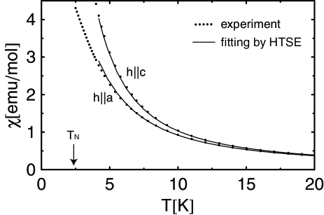
Figure 5: Fitting to susceptibility of MnNi(NO₂)₄(en)₂ by Eq.(18). Here, $(\mu_{\textrm{B}}^{2}N_{\textrm{A}}/k_{\textrm{B}})\chi$ is plotted, where $\mu_{\textrm{B}}$, $N_{\textrm{A}}$ and $k_{\textrm{B}}$ are Bohr magneton, Avogadro’s number and Boltzmann constant, respectively.

In Ref. Feyerherm01, , values of $J\sim 1.9\textrm{K}$ and $D\sim-0.45\textrm{K}$ have been reported for MnNi(NO₂)₄(en)₂. These have been obtained by fitting a directional average of the susceptibility with respect to the magnetic field to the ‘half-classical’ limit, Kahn92 i.e. $S\rightarrow\infty$, applicable for $D=0$. Moreover the effects of interchain coupling have been neglected. To compare with this result we may use $J_{\perp}\equiv 0$ in Eq. (18). In fair agreement with Ref. Feyerherm01, , we find $J\sim 2.4\textrm{K}$ and $D\sim-0.36\textrm{K}$ in this case, with a quality of the fit however, which is inferior to that shown on Fig. 5.

V Summary

We have studied the specific heat and uniform susceptibility of mixed-spin chain systems using a combination of high-temperature series expansion, exact diagonalization, and quantum Monte Carlo techniques. In particular, we have contrasted the cases of FM and AFM intra-chain exchange. A symbolic high-temperature series has been derived for general values of the spin quantum numbers, and including single ion anisotropies. Using this series expansion, we were able to extract the microscopic model parameters for the quasi-one-dimensional FM mixed-spin chain compound MnNi(NO₂)₄(en)₂. Comparing our results to the analytically solvable limit $S\rightarrow\infty$, we found that not only the AFM but also the FM case displays a double-peak-like structure in the specific heat which is due to the presence of both ‘optical’ and ‘acoustic’ excitations. In fact, we find that for FM intra-chain coupling this structure is more pronounced than for AFM exchange. The low-temperature specific heat of MnNi(NO₂)₄(en)₂ shows a weak shoulder around 1.5K if magnetic order is suppressed by a finite magnetic field. It is thus suggestive to associate this shoulder with the presence of ‘acoustic’ excitations in this compound. However, a quantitatively accurate description of the relevant temperature range for the FM mixed-spin chain with $s=1$ and $S=5/2$ in a magnetic field requires further numerical studies and is left for future investigations. Finally, comparing the AFM with the FM case in the extreme quantum limit, i.e. $s=1/2$, $S=1$, we found finite-size effects to be more pronounced in the FM than in the AFM case. This suggests long-range collective excitations to be more relevant for the low-temperature thermodynamics of FM mixed-spin chains.

Appendix A Series Data

Using $X\equiv S(S+1)$ and $x\equiv s(s+1)$, the specific heat series without the single-site anisotropy is given by

$$C=C_{\textrm{D}}+C_{\textrm{ND}}(x,X)+C_{\textrm{ND}}(X,x)+O\left[(\beta J)^{12}\right],$$ (19)

$$C_{\textrm{D}} = \frac{2\,x\,X\,(\beta J)^{2}}{3}-\frac{x\,X\,(\beta J)^{3}}{3}+\left(\frac{2\,x\,X}{15}-\frac{2\,x^{2}\,X^{2}}{15}\right)\,(\beta J)^{4}+\left(\frac{-x\,X}{18}+\frac{2\,x^{2}\,X^{2}}{27}\right)\,(\beta J)^{5}$$ (20)

$$+\left(\frac{8\,x\,X}{315}+\frac{643\,x^{2}\,X^{2}}{7560}+\frac{4\,x^{3}\,X^{3}}{189}\right)\,(\beta J)^{6}+\left(\frac{-23\,x\,X}{1800}-\frac{4043\,x^{2}\,X^{2}}{32400}-\frac{2\,x^{3}\,X^{3}}{135}\right)\,(\beta J)^{7}$$

$$+\left(\frac{19\,x\,X}{2700}+\frac{1162\,x^{2}\,X^{2}}{10125}-\frac{622\,x^{3}\,X^{3}}{18225}-\frac{2\,x^{4}\,X^{4}}{675}\right)\,(\beta J)^{8}$$

$$+\left(\frac{-2231\,x\,X}{529200}-\frac{1489333\,x^{2}\,X^{2}}{15876000}+\frac{115043\,x^{3}\,X^{3}}{2976750}+\frac{4\,x^{4}\,X^{4}}{1575}\right)\,(\beta J)^{9}$$

$$+\left(\frac{15901\,x\,X}{5821200}+\frac{15768563\,x^{2}\,X^{2}}{209563200}-\frac{5996723\,x^{3}\,X^{3}}{943034400}+\frac{36427\,x^{4}\,X^{4}}{3742200}+\frac{4\,x^{5}\,X^{5}}{10395}\right)\,(\beta J)^{10}$$

$$+\left(\frac{-72557\,x\,X}{38102400}-\frac{822853\,x^{2}\,X^{2}}{13395375}-\frac{111661717\,x^{3}\,X^{3}}{3857868000}-\frac{1448899\,x^{4}\,X^{4}}{128595600}-\frac{2\,x^{5}\,X^{5}}{5103}\right)\,(\beta J)^{11},$$

$$C_{\textrm{ND}}(x,X) = \frac{-8\,x\,X^{2}\,(\beta J)^{4}}{45}+\frac{4\,x\,X^{2}\,(\beta J)^{5}}{27}+\left(\frac{-179\,x\,X^{2}}{1890}+\frac{2\,x\,X^{3}}{63}+\frac{10\,x^{2}\,X^{3}}{189}\right)\,(\beta J)^{6}$$ (21)

$$+\left(\frac{157\,x\,X^{2}}{2700}-\frac{x\,X^{3}}{25}-\frac{82\,x^{2}\,X^{3}}{2025}\right)\,(\beta J)^{7}$$

$$+\left(\frac{-124\,x\,X^{2}}{3375}+\frac{124\,x\,X^{3}}{3375}-\frac{6091\,x^{2}\,X^{3}}{364500}-\frac{16\,x\,X^{4}}{3375}-\frac{1064\,x^{2}\,X^{4}}{91125}-\frac{8\,x^{3}\,X^{4}}{675}\right)\,(\beta J)^{8}$$

$$+\left(\frac{3229\,x\,X^{2}}{132300}-\frac{1019\,x\,X^{3}}{33075}+\frac{23281\,x^{2}\,X^{3}}{441000}+\frac{8\,x\,X^{4}}{945}+\frac{128\,x^{2}\,X^{4}}{10125}+\frac{244\,x^{3}\,X^{4}}{23625}\right)\,(\beta J)^{9}$$

$$+\left(\frac{-17137\,x\,X^{2}}{997920}+\frac{24727\,x\,X^{3}}{970200}-\frac{86018257\,x^{2}\,X^{3}}{1257379200}-\frac{11489\,x\,X^{4}}{1091475}+\frac{6287\,x^{2}\,X^{4}}{11642400}\right.$$

$$\left.+\frac{25411\,x^{3}\,X^{4}}{2619540}+\frac{4\,x\,X^{5}}{6237}+\frac{316\,x^{2}\,X^{5}}{155925}+\frac{218\,x^{3}\,X^{5}}{66825}+\frac{2\,x^{4}\,X^{5}}{891}\right)\,(\beta J)^{10}$$

$$+\left(\frac{732629\,x\,X^{2}}{57153600}-\frac{757\,x\,X^{3}}{35280}+\frac{11884871\,x^{2}\,X^{3}}{163296000}+\frac{10279\,x\,X^{4}}{893025}-\frac{5676361\,x^{2}\,X^{4}}{367416000}\right.$$

$$\left.-\frac{3918727\,x^{3}\,X^{4}}{214326000}-\frac{1382\,x\,X^{5}}{893025}-\frac{2672\,x^{2}\,X^{5}}{893025}-\frac{30181\,x^{3}\,X^{5}}{8037225}-\frac{32\,x^{4}\,X^{5}}{14175}\right)\,(\beta J)^{11}.$$

We have computed the series of the susceptibility with the single-site anisotropy up to up to $O(\beta^{7})$, which is too lengthy to be fully listed in this paper. Hence, we show here only the first four terms of the series, and the rest will be provided on request. Since the non-commutativity, Eq. (17), is neglected in Ref. Kahn92, , the $S\rightarrow\infty$ limit of the series below with $D=0$ and $g\neq G$ is different from the function given in Ref. Kahn92, .

$$\chi_{zz} = \beta\,\left(\frac{{g}^{2}\,x}{3}+\frac{{G}^{2}\,X}{3}\right)+{\beta}^{2}\,\left\{\frac{4\,g\,G\,J\,x\,X}{9}-D\,{G}^{2}\,\left[\frac{-X}{15}+\frac{4\,X^{2}}{45}\right]\right\}+{\beta}^{3}\,\Bigg{\{}{g}^{2}\,J^{2}\,\left[\frac{-\left(x\,X\right)}{27}+\frac{2\,x^{2}\,X}{27}\right]$$ (22)

$$+g\,G\,\left[\frac{-\left(J^{2}\,x\,X\right)}{27}-D\,J\,\left(\frac{-4\,x\,X}{45}+\frac{16\,x\,X^{2}}{135}\right)\right]+{G}^{2}\,\left[J^{2}\,\left(\frac{-\left(x\,X\right)}{27}+\frac{2\,x\,X^{2}}{27}\right)+{D}^{2}\,\left(\frac{X}{42}-\frac{4\,X^{2}}{105}+\frac{8\,X^{3}}{945}\right)\right]\Bigg{\}}$$

$$+{\beta}^{4}\,\Bigg{\{}{g}^{2}\,\left[J^{3}\,\left(\frac{x\,X}{108}-\frac{x^{2}\,X}{81}\right)-D\,J^{2}\,\left(\frac{2\,x\,X}{675}-\frac{16\,x^{2}\,X}{675}-\frac{8\,x\,X^{2}}{2025}+\frac{64\,x^{2}\,X^{2}}{2025}\right)\right]+g\,G\,\left[D\,J^{2}\,\left(\frac{4\,x\,X^{2}}{405}-\frac{x\,X}{135}\right)\right.$$

$$\left.+J^{3}\,\left(\frac{x\,X}{90}-\frac{16\,x^{2}\,X}{405}-\frac{16\,x\,X^{2}}{405}+\frac{8\,x^{2}\,X^{2}}{405}\right)+{D}^{2}\,J\,\left(\frac{2\,x\,X}{63}-\frac{16\,x\,X^{2}}{315}+\frac{32\,x\,X^{3}}{2835}\right)\right]$$

$$+{G}^{2}\,\left[J^{3}\,\left(\frac{x\,X}{108}-\frac{x\,X^{2}}{81}\right)-D\,J^{2}\,\left(\frac{x\,X}{54}-\frac{22\,x\,X^{2}}{405}+\frac{16\,x\,X^{3}}{405}\right)-{D}^{3}\,\left(\frac{-X}{90}+\frac{97\,X^{2}}{4725}-\frac{32\,X^{3}}{4725}-\frac{16\,X^{4}}{14175}\right)\right]\Bigg{\}}$$

$$+\ldots,$$

$$\chi_{xx} = \beta\,\left(\frac{{g}^{2}\,x}{3}+\frac{{G}^{2}\,X}{3}\right)+{\beta}^{2}\,\left\{\frac{4\,g\,G\,J\,x\,X}{9}-D\,{G}^{2}\,\left(\frac{X}{30}-\frac{2\,X^{2}}{45}\right)\right\}+{\beta}^{3}\,\Bigg{\{}{g}^{2}\,J^{2}\,\left[\frac{-\left(x\,X\right)}{27}+\frac{2\,x^{2}\,X}{27}\right]$$ (23)

$$+g\,G\,\left[\frac{-\left(J^{2}\,x\,X\right)}{27}-D\,J\,\left(\frac{2\,x\,X}{45}-\frac{8\,x\,X^{2}}{135}\right)\right]+{G}^{2}\,\left[J^{2}\,\left(\frac{-\left(x\,X\right)}{27}+\frac{2\,x\,X^{2}}{27}\right)+{D}^{2}\,\left(\frac{X}{210}-\frac{X^{2}}{315}-\frac{4\,X^{3}}{945}\right)\right]\Bigg{\}}$$

$$+{\beta}^{4}\,\Bigg{\{}{g}^{2}\,\left[J^{3}\,\left(\frac{x\,X}{108}-\frac{x^{2}\,X}{81}\right)-D\,J^{2}\,\left(\frac{-\left(x\,X\right)}{675}+\frac{8\,x^{2}\,X}{675}+\frac{4\,x\,X^{2}}{2025}-\frac{32\,x^{2}\,X^{2}}{2025}\right)\right]$$

$$+g\,G\,\left[D\,J^{2}\,\left(\frac{x\,X}{270}-\frac{2\,x\,X^{2}}{405}\right)+J^{3}\,\left(\frac{x\,X}{90}-\frac{16\,x^{2}\,X}{405}-\frac{16\,x\,X^{2}}{405}+\frac{8\,x^{2}\,X^{2}}{405}\right)\right.$$

$$\left.+{D}^{2}\,J\,\left(\frac{2\,x\,X}{315}-\frac{4\,x\,X^{2}}{945}-\frac{16\,x\,X^{3}}{2835}\right)\right]+{G}^{2}\,\left[J^{3}\,\left(\frac{x\,X}{108}-\frac{x\,X^{2}}{81}\right)-D\,J^{2}\,\left(\frac{-\left(x\,X\right)}{108}+\frac{11\,x\,X^{2}}{405}-\frac{8\,x\,X^{3}}{405}\right)\right.$$

$$\left.-{D}^{3}\,\left(\frac{-X}{2520}-\frac{X^{2}}{1350}+\frac{2\,X^{3}}{1575}+\frac{8\,X^{4}}{14175}\right)\right]\Bigg{\}}+\ldots.$$

References

- (1) O. Kahn, Y. Pei, and Y. Journaux, in Inorganic Materials, edited by D. W. Bruce and D. O’Hare (Wiley, New York, 1996), p. 65.
- (2) A. Caneschi, D. Gatteschi, J.-P. Renard, P. Rey and R. Sessoli, Inorg. Chem. 28, 2940 (1989).
- (3) M. Nishizawa, D. Shiomi, K. Sato, T. Takui, K. Itoh, H. Sawa, R. Kato, H. Sakurai, A. Izuoka, and T. Sugawara, J. Phys. Chem. B 104, 503 (2000).
- (4) S. K. Pati, S. Ramasesha, and D. Sen, Phys. Rev. B 55, 8894 (1997).
- (5) S. K. Pati, S. Ramasesha, and D. Sen, J. Phys.: Condens. Matter 9, 8707 (1997).
- (6) S. Brehmer, H.-J. Mikeska, and S. Yamamoto, J. Phys.: Condens. Matter 9, 3921 (1997).
- (7) S. Yamamoto, S. Brehmer, and H.-J. Mikeska, Phys. Rev. B 57, 13610 (1998).
- (8) S. Yamamoto and T. Fukui, Phys. Rev. B 57, R14008 (1998).
- (9) S. Yamamoto, T. Fukui, K. Maisinger, and U. Schollwöck, J. Phys.: Condensed Matter 10, 11033 (1998).
- (10) S. Yamamoto and T. Sakai, J. Phys. Soc. Japan 67, 3711 (1998).
- (11) A.K. Kolezhuk, H.-J. Mikeska, and S. Yamamoto, Phys. Rev. B 55, R3336 (1997).
- (12) T. Nakanishi and S. Yamamoto, Phys. Rev. B 65, 214418 (2002).
- (13) R. Feyerherm, C. Mathonière, and O. Kahn, J. Phys. Condens. Matter 13, 2639 (2001).
- (14) S. T. Dembiński and T. Wydro, phys. stat. sol. (b) 67, K123 (1975).
- (15) J. Seiden, J. Phys. (Paris) Lett. 44, L947 (1983).
- (16) O. Kahn, Y. Pei, K. Nakatani, Y. Journaux, and J. Sletten, New J. Chem. 16, 269 (1992).
- (17) G. S. Rushbrooke, G. A. Baker Jr., and P. J. Wood, in Phase Transitions and Critical Phenomena, edited by C. Domb and M. S. Green (Academic, London, 1974), vol.3, p.245.
- (18) G. A. Baker Jr., G. S. Rushbrooke, and H. E. Gilbert, Phys. Rev. 135, A1272 (1964).
- (19) N. Fukushima, J. Stat. Phys. 111, 1049 (2003).
- (20) In a finite field, the correction term is replaced by , and the other terms are the same.
- (21) e.g. Mathematica
- (22) M. Takahashi and M. Yamada, J. Phys. Soc. Japan 54, 2808 (1985).
- (23) B. Bernu and G. Misguich, Phys. Rev. B 63, 134409 (2001).
- (24) A. W. Sandvik, Phys. Rev. B 59, R14157 (1999).
- (25) P. J. Wojtowicz, Phys. Rev. 155, 492 (1967).
- (26) S. Freeman and P. J. Wojtowicz, Phys. Rev. B 6, 304 (1972).
- (27) The series coefficients listed in Fig. 2 in Ref. Wojtowicz67, are not consistent with that of the uniform systemBaker64 ; Rushbrooke58 , i.e. the case. Most likely, “” in the table should be replaced by “”.
- (28) R. Feyerherm (private communication).
- (29) G. S. Rushbrooke and P. J. Wood, Mol. Phys. 1, 257 (1958).