Generalization of the Hartree-Fock-Bogoliubov theory: one and two quasiparticle excitations

Abstract

We present a generalization of the Hartree-Fock Bogoliubov (HFB) theory in which the coupling between one and two quasi-particles is taken into account.This is done by writing the excitation operators as linear combinations of one and two HFB quasi-particles. The excitation energies and the quasi-particle amplitudes are given by generalized Bogoliubov equations. The excitation spectrum has two branches. The first one is a discrete branch which is gapless and has a phonon character at large wave-length and, contrarily to HFB, is always stable. This branch is detached from a continuum branch whose threshold, at fixed total momentum, coincides with the two quasi-particle threshold of the HFB theory. The gap between these two branches at P=0 is equal to two times the HFB gap, which then provides for the relevant energy scale. We also give numerical results for a specific case.

I Introduction

The experimental realization of Bose-Einstein condensation in trapped neutral bosonic atoms has opened the opportunity for a comparison of microscopic theories of dilute systems with experimental data 1 . The standard approach is to solve the Gross-Pitaevskii (GP) equation for the condensate wave function and the linear Bogoliubov-de Gennes (BdG) equations for the collective excitations 2 . For $T=0$ this theory has been successfully compared with the existing data 3 -5 .
Physically, the GP + BdG theory is a free quasi-particles theory. However it is not the best of such theory from a variational point of view, being superseded by the Hartree-Fock- Bogoliubov (HFB) theory 6 , where the non-linear BdG equations are solved self-consistently and the GP and BdG equations are coupled. The two approaches agree when we neglect the depletion of the condensate in the self-consistent theory. This would suggest that HFB is the proper theory to use when the fluctuations become important, for example, in trapped gases through the mechanism of Feshbach resonance 7 or at finite temperature. It is however well known that the HFB theory has problems when applied to homogeneous systems 6 . Indeed, the excitation spectrum has a gap which violates the Hugenholtz-Pines theorem, which states that the excitation spectrum should be gapless 8 . The HFB theory is also in contradiction with some thermodynamic data in ⁴He (for example, the specific heat), which requires that, in the large wave-length limit, the excitation spectrum should have a phonon behavior 9 .

In this paper we present a generalization of the HFB theory leading to an excitation spectrum which, in particular, eliminates the gap problem. The key ingredient for this is the inclusion of two quasi-particle components together with their coupling to one quasi-particle components for the description of the excitation spectrum. Excitation energies and the structure of the corresponding modes are given by generalized Bogoliubov equations. The excitation spectrum includes a discrete stable phonon-like excitation branch. In addition to this discrete branch there is a continuum branch whose threshold is located at twice the HFB quasi-particle energy. This branch has, therefore, a gap at total momentum ${\bf P}=0$ which is twice the HFB gap. Therefore, this gap sets an important energy scale for the excitation spectrum.

The use of this mechanism to solve the HFB gap problem has in fact being pioneered more than for decades ago by Takano 10 . A more recent work by Hutchinson at al 11 deals with the coupling between one and two quasi-particle components in a perturbative way, while the work of Kerman and Tommasini 12 deals with the same problem on the basis of the Gaussian functional approximation to a field theoretical variational procedure.

In this paper we use standard equations of motion techniques 14 ; 15 , employed, for example, in reference 13 to study chiral symmetry restoration in the linear $\sigma$ model non-pertubatively. This allows for a clear identification of the dynamical role played by various parts of the many-body hamiltonian when expanded in terms of quasi-particles.

Our paper is organized as follows: In section 2 we briefly discuss the basic properties of the HFB theory. In section 3 we derive the generalized Bogoliubov equations for the excitation energies and quasi-particle amplitudes. Our derivation allows for a clear identification of parts of the hamiltonian responsible for the coupling between on and two quasi-particle components of the excitation operator. In section 4, we show that there exist a Goldstone mode at momentum equal to zero. Our proof of its existence is very simple and clearly related to the violation of number conservation. The results of a numerical application of the theory are discussed in section 5. Specifically we examine the properties of the excitation spectrum, its stability, and change in physical content as a function of the total momentum ${\bf P}$. We also make a comparison with the HFB and Bogoliubov approximations. Our conclusions are presented in section 6. All the expressions needed for numerical applications are given in appendices $A$ and $B$.

II The HFB theory

The starting point is the Grand-Hamiltonian written in second quantization as

$$\hat{h}=\hat{H}-\mu\hat{N}=\sum_{\bf k}(e_{k}-\mu)a_{\bf k}^{\dagger}a_{\bf k}+\frac{1}{2}\sum_{\bf k_{1},k_{2},{\bf q}}V(q)a_{{\bf k_{1}}+{\bf q}}^{\dagger}a_{{\bf k_{2}}-{\bf q}}^{\dagger}a_{\bf k_{1}}a_{\bf k_{2}}$$ (1)

where $e_{k}$ is the free particle kinetic energy,

$$e_{k}=\frac{\hbar^{2}k^{2}}{2m},$$ (2)

$V(q)$ is the Fourier transform per unit volume of the atom-atom interaction potential

$$V(q)=\frac{1}{\Gamma}\int V(r)e^{i{\bf q}.{\bf r}}d^{3}r=\frac{\tilde{V}(q)}{\Gamma},$$ (3)

and the operators $a_{\bf k}^{\dagger}$ e $a_{\bf k}$, respectively, create and annihilate atoms in a state with momentum $\hbar{\bf k}$, the corresponding wave-function $\exp(i{\bf k}.{\bf r})/\sqrt{\Gamma}$ satisfying periodic boundary conditions in a cubic box of volume $\Gamma$.

In a first step we perform a canonical transformation to the quasi-particles by introducing a new set of creation and annihilation operators through the Bogoliubov rotation 16

$$a_{\bf k}=c_{\bf k}+z_{0}\delta_{{\bf k},0}=u_{\bf k}\eta_{\bf k}-v_{\bf k}\eta_{-\bf k}^{\dagger}+z_{0}\delta_{{\bf k},0},$$ (4)

where $u_{\bf k}$ and $v_{\bf k}$ are even functions of ${\bf k}$, $u_{\bf k}=u_{-{\bf k}}$, $v_{\bf k}=v_{-{\bf k}}$, and $z_{0}$ is a c-number. The constant $z_{0}$ appears as a shift in the equation for ${\bf k}=0$ to account for the macroscopic condensate in the zero momentum state. In order to render the transformation canonical, the Bogoliubov factors have to obey the constraint

$$u_{\bf k}^{2}-v_{\bf k}^{2}=1.$$ (5)

It is straightforward to write the Grand-Hamiltonian $\hat{h}$ in the quasi-particle basis. After normal ordering one obtains,

$$\hat{h}=\hat{H}-\mu\hat{N}=h_{0}+\hat{h}_{1}+\hat{h}_{2}+\hat{h}_{3}+\hat{h}_{4}$$ (6)

where the normal ordered operators $\hat{h_{i}}$ contain $i$ quasi-particles. They are written explicitly in Appendix A.

The amplitudes $u_{\bf k}$, $v_{\bf k}$ and the shift $z_{0}$ are determined in the HFB theory by minimizing the expectation value of $\hat{h}$, $\langle\Phi|\hat{h}|\Phi\rangle$ in the quasi-particle vacuum, that is, $\eta_{\bf k}|\Phi\rangle=0$. Since the only term which contributes to the expectation value is the term $h_{0}$, the minimization is equivalent to the equations

$$\frac{\partial h_{0}}{\partial z_{0}} = 0$$ (7)

$$\frac{\partial h_{0}}{\partial v_{\bf k}}+\frac{\partial h_{0}}{\partial u_{\bf k}}\frac{\partial u_{\bf k}}{\partial v_{\bf k}} = 0$$ (8)

with $h_{0}$ given by

$$h_{0} = -z_{0}^{2}\mu+\frac{z_{0}^{4}}{2}V(0)+\sum_{\bf k}[e_{k}-\mu+(V(0)+V(k))z_{0}^{2}]v_{\bf k}^{2}$$ (9)

$$-\sum_{\bf k}V(k)z_{0}^{2}u_{\bf k}v_{\bf k}+\frac{1}{2}\sum_{{\bf k_{1}},{\bf k_{2}}}(V(0)+V(|{\bf k_{1}}-{\bf k_{2}}|)v_{\bf k_{1}}^{2}v_{\bf k_{2}}^{2}$$

$$+\frac{1}{2}\sum_{{\bf k_{1}},{\bf k_{2}}}V(|{\bf k_{1}}-{\bf k_{2}}|)u_{\bf k_{1}}v_{\bf k_{1}}u_{\bf k_{2}}v_{\bf k_{2}}$$

The two equations above can be written in a very compact way if we introduce the Hartree, exchange and pair potentials defined by the following relations 17 :

$${U}_{h} = \sum_{\bf k_{1}}V(0)\langle\Phi|a_{\bf k_{1}}^{\dagger}a_{\bf k_{1}}|\Phi\rangle$$ (10)

$${U}_{ex}(\bf k) = \sum_{\bf k_{1}}V(|{\bf k}-{\bf k_{1}}|)\langle\Phi|a_{\bf k_{1}}^{\dagger}a_{\bf k_{1}}|\Phi\rangle$$ (11)

$${U}_{pair}(\bf k) = \sum_{\bf k_{1}}V(|{\bf k}-{\bf k_{1}}|)\langle\Phi|a_{\bf k_{1}}a_{-\bf k_{1}}|\Phi\rangle$$ (12)

These potentials can be written as the sum of two terms which can be interpreted as related to the condensate and to the non-condensate, respectively

$${U}_{h} = U_{h}^{c}+U_{h}^{nc}=V(0)z_{0}^{2}+\sum_{\bf k_{1}}V(0)\langle\Phi|c_{\bf k_{1}}^{\dagger}c_{\bf k_{1}}|\Phi\rangle$$ (13)

$${U}_{ex}(\bf k) = U_{ex}^{c}+U_{ex}^{nc}=V(k)z_{0}^{2}+\sum_{\bf k_{1}}V(|{\bf k}-{\bf k_{1}}|)\langle\Phi|c_{\bf k_{1}}^{\dagger}c_{\bf k_{1}}|\Phi\rangle$$ (14)

$${U}_{pair}(\bf k) = U_{pair}^{c}+U_{pair}^{nc}=V(k)z_{0}^{2}+\sum_{\bf k_{1}}V(|{\bf k}-{\bf k_{1}}|)\langle\Phi|c_{\bf k_{1}}c_{-\bf k_{1}}|\Phi\rangle$$ (15)

In terms of these potentials the equilibrium equations (7) and (8) can be written as

$$z_{0}[-\mu+{U}_{h}+{U}_{ex}^{nc}(0)+{U}_{pair}^{nc}(0)]=0$$ (16)

$$\tanh 2\sigma_{k}=\frac{{U}_{pair}(\bf k)}{e_{k}+{U}_{h}+{U}_{ex}(\bf k)-\mu}=\frac{{U}_{pair}(\bf k)}{\tilde{e}(\bf k)},$$ (17)

with $u_{\bf k}=\cosh\sigma_{\bf k}$ and $v_{\bf k}=\sinh\sigma_{\bf k}$.

The quasi-particle vacuum $|\Phi\rangle$ does not have a definite number of particles. In order to control the number of particles we determine $\mu$ from the condition that the mean value of the number of particles in the state $|\Phi\rangle$ is $N$, $N=\langle\Phi|\hat{N}|\Phi\rangle$ which gives

$$N=z_{0}^{2}+\sum_{\bf k}v_{\bf k}^{2}$$ (18)

Thus, the set of equations (16), (17) and (18) determine $\mu$, $z_{0}$ and the Bogoliubov amplitudes $u_{\bf k}$ and $v_{\bf k}$. Equations ( 16) and (17) can also be derived by demanding that $\hat{h}_{1}$ vanishes and that $\hat{h}_{2}$ is diagonal in the quasi-particle basis, $\hat{h}_{2}=\sum_{\bf k}\omega({\bf k})\eta_{\bf k}^{\dagger}\eta_{\bf k}$, with $\omega({\bf k})$ the quasi-particle energies, $\omega({\bf k})^{2}=\tilde{e}({\bf k})^{2}-{U}_{pair}(\bf k)^{2}$.

One feature of the HFB theory is that the excitation energy have a gap in the limit $k\rightarrow 0$ 6 ,

$$\omega(0)^{2}=-4\tilde{V}(0)n_{0}{U}_{pair}^{nc}(0)$$ (19)

where $n_{0}=z_{0}^{2}/\Gamma$ is the condensate density. The existence of an energy gap in the excitation spectrum does not agree with the phonon spectrum in superfluid systems and is also in contradiction with the Hugenholtz-Pines (HP) 8 theorem, which sates that the energy of an excitation with wavenumber ${\bf k}$ of a many-body system should vanish when $k\rightarrow 0$.

An approximate way to satisfy the HP theorem is to neglect the so-called anomalous density $m_{\bf k}=\langle\Phi|c_{\bf k}c_{-\bf k}|\Phi\rangle$ in the HFB theory 6 . In this approximation $U_{pair}^{nc}(\bf k)$ vanishes and the gap disappears. This approximation is known as the Popov approximation. In the next section we are going to present a theory that has a gapless dispersion relation while taking $m_{\bf k}$ fully into account. As it turns out, this theory also gives a physical meaning to (19).

III The quasi-particle RPA

As is well known in many-body physics the Random Phase Approximation (RPA) singles out the Goldstone mode due to a symmetry breaking at the mean field level 14 ; 15 .

One among the many ways of deriving the RPA equations, is the linearization of the equations of motion 21 . In principle, if we find operators satisfying the equations

$$[H,Q_{\alpha}^{\dagger}] = \Omega_{\alpha}Q_{\alpha}^{\dagger}$$ (20)

$$Q_{\alpha}|\Psi_{0}\rangle = 0$$ (21)

with the normalization condition

$$\langle\Psi_{0}|[Q_{\beta},Q_{\alpha}^{\dagger}]|\Psi_{0}\rangle=\delta_{\beta,\alpha}$$ (22)

where $|\Psi_{0}\rangle$ is the exact ground state, we have found an exact excited state of the many-body system since, from the above equations, it follows that $|\Psi_{\alpha}\rangle=Q_{\alpha}^{\dagger}|\Psi_{0}\rangle$ is an eigenstate of H with excitation energy equal to $\Omega_{\alpha}$. However this cannot be carried out in general, and we are bound to use approximate methods regarding both $Q_{\alpha}$ and $|\Psi_{0}\rangle$ in the solution of equations (20) and (21). In the method of the linearization of the equations of motion we make an ansatz about the form of the excitation operators, writing it as a linear combination of basic excitations and we linearize the left -hand side of equation (20) with respect to these operators.

In this paper we look for excitation operators which are a combination of one and two HFB quasi-particles,

$$Q_{\bf P}^{\dagger}=x_{\bf P}\eta_{\bf P}^{\dagger}+y_{\bf P}\eta_{-\bf P}+\sum_{{\bf q}\geq 0}X_{{\bf q},{\bf P}}\frac{\eta_{{\bf q}+{\bf P}/2}^{\dagger}\eta_{-{\bf q}+{\bf P}/2}^{\dagger}}{\sqrt{1+\delta_{{\bf q},0}}}+Y_{{\bf q},{\bf P}}\frac{\eta_{-{\bf q}-{\bf P}/2}\eta_{{\bf q}-{\bf P}/2}}{\sqrt{1+\delta_{{\bf q},0}}}$$ (23)

In the equation (23) $Q_{\bf P}^{\dagger}$ creates an excitation with momentum ${\bf P}$ and it is a linear combination of one, $\eta_{\bf P}^{\dagger}$, $\eta_{-\bf P}$ , and two, $\eta_{{\bf q}+{\bf P}/2}^{\dagger}\eta_{-{\bf q}+{\bf P}/2}^{\dagger}$, $\eta_{-{\bf q}-{\bf P}/2}\eta_{{\bf q}-{\bf P}/2}$ HFB quasi- particles. This last term creates (annihilates) a pair with total momentum ${\bf P}(-{\bf P})$ and relative momentum $\bf q$. The coefficients $x_{\bf P}$, $y_{\bf P}$, $X_{{\bf q},{\bf P}}$ and $Y_{{\bf q},{\bf P}}$ are even functions of $\bf P$. As the pair creation and annihilation are invariant by the replacement ${\bf q}\rightarrow-{\bf q}$, $X_{{\bf q},{\bf P}}$ and $Y_{{\bf q},{\bf P}}$ are even functions of $\bf q$ and we restrict the sum in order that the pairs appear only once.

The coefficients in (23) are determined by the method of the equations of motion in the version of references 14 and 15 , which is a systematic way of achieving the linearization referred above. Following these references, notice that from equations (20) and (21) one has

$$\langle\Psi_{0}|[Q_{\bf P},H,Q_{\bf P}^{\dagger}]|\Psi_{0}\rangle=\Omega_{P}\langle\Psi_{0}|[Q_{\bf p},Q_{\bf P}^{\dagger}]|\Psi\rangle$$ (24)

where $[A,B,C]$ is the symmetrized double commutator $\frac{1}{2}([A,[B,C]]+[[A,B],C])$.

Requiring that $\Omega_{\bf P}$ be stationary in a variation of the excitation operators one has:

$$\langle\Phi|[\delta Q_{\bf P},H,Q_{\bf P}^{\dagger}]|\Phi\rangle=\Omega_{P}\langle\Phi|[\delta Q_{\bf p},Q_{\bf P}^{\dagger}]|\Phi\rangle$$ (25)

where $\delta Q_{\bf P}$ is the hermitian conjugate of the operator given by the variation of the coefficients in (23) and, as usual, we replaced the ground state $|\Psi_{0}\rangle$ by the HFB vacuum , $|\Phi\rangle$.

Performing the variation indicated in equation (25), we get for the excitation energies $\Omega_{P}$ and the coefficients

$${\cal X}=\left(\begin{array}[]{c}x_{\bf P}\\ X_{\bf P}\end{array}\right)\quad\mbox{and}\quad{\cal Y}=\left(\begin{array}[]{c}y_{\bf P}\\ Y_{\bf P}\end{array}\right),$$ (26)

the equation

$$\left(\begin{array}[]{cc}{\cal A}&{\cal B}\\ {{\cal B}^{\ast}}&{\cal A}^{\ast}\end{array}\right)\left(\begin{array}[]{c}{\cal X}\\ {\cal Y}\end{array}\right)=\Omega_{P}\left(\begin{array}[]{cc}1&0\\ 0&-1\end{array}\right)\left(\begin{array}[]{c}{\cal X}\\ {\cal Y\par}\end{array}\right),$$ (27)

with the coefficients obeying the normalization condition

$$\langle\Phi|[Q_{\bf P}^{\lambda},Q_{\bf P}^{\dagger^{\tau}}]\Phi\rangle=x_{\bf P}^{\lambda^{\ast}}x_{\bf P}^{\tau}-y_{\bf P}^{\lambda^{\ast}}y_{\bf P}^{\tau}+\sum_{{\bf q}\geq 0}\left(X_{{\bf q},{\bf P}}^{\lambda^{\ast}}X_{{\bf q},{\bf P}}^{\tau}-Y_{{\bf q},{\bf P}}^{\lambda^{\ast}}Y_{{\bf q},{\bf P}}^{\tau}\right)=\delta_{\lambda,\tau}.$$ (28)

For each P we have a number of modes equal to the number of operator pairs plus one, $n_{\mbox{p}airs}+1$, actually this number is denumerable infinite, and this is denoted by the quantum numbers $\lambda$, $\tau$ in equation (28).

In expression (26), $X_{\bf P}(Y_{\bf P})$ stands for the set of $n_{\mbox{p}airs}$ coefficients $X_{{\bf q},{\bf P}}(Y_{{\bf q},{\bf P}})$ and ${\cal A}$ and ${\cal B}$ are, respectively, hermitian and symmetric matrices of dimension $n_{\mbox{p}airs}+1$.

The hermitian matrix ${\cal A}$ is given by

$${\cal A}=\left(\begin{array}[]{cc}{\cal A}^{11}&{\cal A}^{12}\\ {\cal A}^{21}&{\cal A}^{22}\end{array}\right).$$ (29)

The diagonal blocks ${\cal A}^{11}$ and ${\cal A}^{22}$ are hermitian matrices with dimensionality 1 and $n_{\mbox{p}airs}$ respectively. They are given by

$${\cal A}^{11}({\bf P})=\langle\Phi|[\eta_{\bf P},H,\eta_{\bf P}^{\dagger}]|\Phi\rangle,$$ (30)

and

$${\cal A}^{22}({\bf q^{\prime}},{\bf q};{\bf P})=\langle\Phi|[\frac{\eta_{{\bf q^{\prime}}+{\bf P}/2}\eta_{-{\bf q^{\prime}}+{\bf P}/2}}{\sqrt{1+\delta_{{\bf q^{\prime}},0}}},H,\frac{\eta_{{\bf q}+{\bf P}/2}^{\dagger}\eta_{-{\bf q}+{\bf P}/2}^{\dagger}}{\sqrt{1+\delta_{{\bf q},0}}}|\Phi\rangle.$$ (31)

The coupling matrices ${\cal A}^{12}$ and ${\cal A}^{21}$ are hermitian conjugates with dimensions $1\times n_{\mbox{p}airs}$ and $n_{\mbox{p}airs}\times 1$ respectively and are given by

$${\cal A}^{12}({\bf q};{\bf P})=\langle\Phi|[\eta_{\bf P},H,\frac{\eta_{{\bf q}+{\bf P}/2}^{\dagger}\eta_{-{\bf q}+{\bf P}/2}^{\dagger}}{\sqrt{1+\delta_{{\bf q},0}}}]|\Phi\rangle,$$ (32)

The symmetric matrix ${\cal B}$ can be split in a similar way

$${\cal B}=\left(\begin{array}[]{cc}{\cal B}^{11}&{\cal B}^{12}\\ {\cal B}^{21}&{\cal B}^{22}\end{array}\right).$$ (33)

The diagonal blocks ${\cal B}^{11}$ and ${\cal B}^{22}$ are symmetric matrices whose elements are given by

$${\cal B}^{11}({\bf P})=\langle\Phi|[\eta_{\bf P},H,\eta_{\bf-P}]|\Phi\rangle,$$ (34)

and

$${\cal B}^{22}({\bf q^{\prime}},{\bf q};{\bf P})=\langle\Phi|[\frac{\eta_{{\bf q^{\prime}}+{\bf P}/2}\eta_{-{\bf q^{\prime}}+{\bf P}/2}}{\sqrt{1+\delta_{{\bf q^{\prime}},0}}},H,\frac{\eta_{-{\bf q}-{\bf P}/2}\eta_{{\bf q}-{\bf P}/2}}{\sqrt{1+\delta_{{\bf q},0}}}|\Phi\rangle.$$ (35)

The coupling matrices ${\cal B}^{12}$ and ${\cal B}^{21}$ are transpose of each other and given by

$${\cal B}^{12}({\bf q};{\bf P})=\langle\Phi|[\eta_{\bf P},H,\frac{\eta_{-{\bf q}-{\bf P}/2}\eta_{{\bf q}-{\bf P}/2}}{\sqrt{1+\delta_{{\bf q},0}}}]|\Phi\rangle,$$ (36)

Note that the matrices 12 and 21 couple one and two quasi-particle excitations whereas the matrices 11 and 22 act only inside the one and two quasi-particle basis, respectively. As shown in appendix B, the matrices 12 and 21 depend only on $\hat{h}_{3}$, (see Eq. 6). Therefore this term is responsible for the coupling between the one and two quasi-particle components. On the other hand the matrices 11 and 22, that do not mix these two components, depend only on $\hat{h}_{2}$ and $\hat{h}_{4}$. All the matrix elements are computed in detail in appendix B.

If the coupling terms $\hat{h}_{3}$ and $\hat{h}_{4}$ are set to zero we have that ${\cal B}=0$ and ${\cal A}$ is diagonal with eigenvalues $\omega({\bf P})$ and $\omega_{2}({\bf q},{\bf P})=\omega({\bf q}+{\bf P}/2)+\omega({-\bf q}+{\bf P}/2)$ which correspond to one and two free quasi-particle energies.

As the static quantities are real, the elements of the matrices ${\cal A}$ and ${\cal B}$ are real and the RPA equations can be written in a more compact and symmetrical form if we introduce the following new variables:

$$\phi_{1}({\bf P}) = x_{\bf P}+y_{\bf P}$$

$$\phi_{2}({\bf q};{\bf P}) = X_{{\bf q},{\bf P}}+Y_{{\bf q},{\bf P}}$$

$$\pi_{1}({\bf P}) = ({x_{\bf P}-y_{\bf P}})$$

$$\pi_{2}({\bf q};{\bf P}) = ({X_{{\bf q},{\bf P}}-Y_{{\bf q},{\bf P}}})$$ (37)

Grouping $\phi_{1}$,$\phi_{2}$ and $\pi_{1}$, $\pi_{2}$ in order to have the following $n_{\mbox{pairs}}+1$ column matrices

$${\cal Q}=\left(\begin{array}[]{c}\phi_{1}({\bf P})\\ \phi_{2}({\bf q};{\bf P})\end{array}\right)\;\;\;\;\;\ {\cal P}=\left(\begin{array}[]{c}\pi_{1}({\bf P})\\ \pi_{2}({\bf q};{\bf P})\end{array}\right)$$ (38)

we can rewrite the equations (27) in a very compact form 11 ; 12

$$\Omega{\cal Q} = {\cal A}_{-}{\cal P}$$ (39)

$$\Omega{\cal P} = {\cal A}_{+}{\cal Q}$$ (40)

where now we work with two symmetric matrices ${\cal A}_{+}$ and ${\cal A}_{-}$ which are given in terms of the matrices ${\cal A}$ and ${\cal B}$ as

$${\cal A}_{+} = {\cal A}+{\cal B}$$ (41)

$${\cal A}_{-} = {\cal A}-{\cal B}$$ (42)

The elements of these matrices can be written as:

$${\cal A}_{-}^{11}={\cal A}_{+}^{11}=\omega({\bf P})$$ (43)

$${\cal A}_{-}^{12}({\bf q},{\bf P})=\frac{z_{0}}{\sqrt{1+\delta_{{\bf q},0}}}C_{0}({\bf P})\{C_{0}(-)C_{0}(+)[V(+)+V(-)]+[C_{0}(+)C_{0}(-)$$

$$-C_{0}^{-1}(+)C_{0}^{-1}(-)]V({\bf P})\}$$ (44)

$${\cal A}_{+}^{12}({\bf q},{\bf P})=\frac{z_{0}}{2\sqrt{1+\delta_{{\bf q},0}}}C_{0}^{-1}({\bf P})\{[C_{0}^{-1}(+)C_{0}(-)+C_{0}(+)C_{0}^{-1}(-)][V(+)+$$

$$V(-)]\}$$ (45)

$${\cal A}_{-}^{22}({\bf q},{\bf q}^{\prime},{\bf P})=[\omega(+)+\omega(-)]\delta_{{\bf q},{\bf q}^{\prime}}+$$

$$\frac{1}{2\sqrt{(1+\delta_{{\bf q},0})(1+\delta_{{\bf q}^{\prime},0})}}\{[C_{0}^{-1}(+^{\prime})C_{0}^{-1}(-^{\prime})C_{0}^{-1}(+)C_{0}^{-1}(-)$$

$$+C_{0}(+^{\prime})C_{0}(-^{\prime})C_{0}(+)C_{0}(-)][V(|{\bf q}-{\bf q}^{\prime}|)+V(|{\bf q}+{\bf q}^{\prime})]+[C_{0}^{-1}(+^{\prime})C_{0}^{-1}(-^{\prime})-$$

$$C_{0}(+^{\prime})C_{0}(-^{\prime})][C_{0}^{-1}(+)C_{0}^{-1}(-)-C_{0}(+)C_{0}(-)]V({\bf P})\}$$ (46)

$${\cal A}_{+}^{22}({\bf q},{\bf q}^{\prime},{\bf P})=[\omega(+)+\omega(-)]\delta_{{\bf q},{\bf q}^{\prime}}+$$

$$\frac{1}{2\sqrt{(1+\delta_{{\bf q},0})(1+\delta_{{\bf q}^{\prime},0})}}[C_{0}^{-1}(+^{\prime})C_{0}(-^{\prime})C_{0}^{-1}(+)C_{0}(-)+$$

$$C_{0}(+^{\prime})C_{0}^{-1}(-^{\prime})C_{0}(+)C_{0}^{-1}(-)]V(|{\bf q}-{\bf q}^{\prime}|)+[C_{0}^{-1}(+^{\prime})C_{0}(-^{\prime})C_{0}^{-1}(-)C_{0}(+)+$$

$$C_{0}(+^{\prime})C_{0}^{-1}(-^{\prime})C_{0}(-)C_{0}^{-1}(+)]V(|{\bf q}+{\bf q}^{\prime}|).$$ (47)

These expressions show the remarkable result that all the matrix elements depend on the static factors through only one function i.e.

$$C_{0}({\bf q})=u_{\bf q}-v_{\bf q}$$ (48)

where we used the notation $\pm=\pm{\bf q}+{\bf P}/2$ and $\pm^{\prime}=\pm{\bf q}^{\prime}+{\bf P}/2$. By solving the coupled equations (39) and (40) we will find the new excitations which will now have one and two quasi-particle contributions. The results for the excitation energies will lead to a discrete branch and a continuum whose threshold coincides with the two quasi-particle threshold of the HFB theory. The discrete branch is detached from the continuum and due to the coupling between the one and two quasi-particles will be pushed down and become gapless. This fact can be proved for any pseudo-potential as will be shown in the next section

IV The Goldstone Mode

Equations (27) have a zero energy solution when ${\bf P}=0$, $\Omega_{0}=0$, with zero-norm, the Goldstone mode 18 . To identify this solution one has to consider the generator of the symmetry violated by the theory which, in our case, is the $U(1)$ symmetry whose generator is the number operator. This operator when written in the HFB basis possesses components that are present in the general ”anzatz” for the excitation operators, eq.(23). These components will be identified with the excitation operator of the Goldstone mode $\hat{Q}_{G}$.

Thus to find $\hat{Q}_{G}$ we start writing the number operator

$$\hat{N}=\sum_{\bf k}a_{\bf k}^{\dagger}a_{\bf k}$$ (49)

in terms of the HFB quasi-particles $\eta_{\bf k}^{\dagger}$, $\eta_{\bf k}$, giving

$$\hat{N}=N+z_{0}(u_{0}-v_{0})(\eta_{0}+\eta_{0}^{\dagger})-\sum_{{\bf k}\geq 0}\frac{2u_{\bf k}v_{\bf k}}{1+\delta_{{\bf k},0}}(\eta_{\bf k}^{\dagger}\eta_{-{\bf k}}^{\dagger}+\eta_{\bf k}\eta_{-{\bf k}})+\sum_{\bf k}(u_{\bf k}^{2}+v_{\bf k}^{2})\eta_{\bf k}^{\dagger}\eta_{\bf k}.$$ (50)

Comparing with the general ”anzatz” eq.(23) we identify the excitation operator of the Goldstone mode with

$$\hat{Q}_{G}=z_{0}(u_{0}-v_{0})(\eta_{0}+\eta_{0}^{\dagger})-\sum_{{\bf k}\geq 0}\frac{2u_{\bf k}v_{\bf k}}{1+\delta_{{\bf k},0}}(\eta_{\bf k}^{\dagger}\eta_{-{\bf k}}^{\dagger}+\eta_{\bf k}\eta_{-{\bf k}}).$$ (51)

Given this form, our next task is to prove that, when ${\bf P}=0$, there is a zero-energy solution of (27) of zero norm with,

$$x_{0} = y_{0}=z_{0}(u_{0}-v_{0})$$ (52)

$$X_{{\bf q},0} = Y_{{\bf q},0}=-\frac{2u_{\bf q}v_{\bf q}}{\sqrt{1+\delta_{{\bf q},0}}}.$$ (53)

Equation (27) is equivalent to the coupled equations (39) and (40). Since the Goldstone mode has zero-energy and zero-norm one has $\Omega_{0}=0$ and ${\cal P}=0$ and the coupled equations reduce to

$${\cal A}_{+}{\cal Q}_{G}=0$$ (54)

with

$${\cal Q}_{G}=\left(\begin{array}[]{c}\phi_{1}(0)\\ \phi_{2}({\bf q};0)\end{array}\right)=\left(\begin{array}[]{c}2x_{0}\\ 2X_{{\bf q},0}\end{array}\right)$$ (55)

From the expression of the matrix elements of ${\cal A}_{+}$ , Eqs. (44) and (46) (at ${\bf P}=0$), ${\cal Q}_{G}$ given above is a zero-energy solution of the eqs. (39) and (40) provided the following identities are satisfied

$$\frac{1}{2}\omega_{0}(u_{0}-v_{0})^{2}+U_{pair}^{nc}(0)=0$$ (56)

$$U_{pair}({\bf q})-2\omega_{\bf q}u_{\bf q}v_{\bf q}=0$$ (57)

These identities are easily seen to hold if we use the following relations obeyed by the static quantities:

$$u_{\bf q}^{2}=\frac{1}{2}\left(\frac{\tilde{e}_{\bf q}}{\omega_{q}}+1\right),\;\;\;\;v_{\bf q}^{2}=\frac{1}{2}\left(\frac{\tilde{e}_{\bf q}}{\omega_{\bf q}}-1\right),$$ (58)

$$2u_{\bf q}v_{\bf q}=\frac{U_{pair}({\bf q})}{\omega_{\bf q}}.$$ (59)

In the equations of motion method the connection between the Goldstone mode excitation operator $\hat{{\cal Q}}_{G}$ and the number operator $\hat{N}$ goes as follows. Since $[\hat{h},\hat{N}]=0$ one has

$$\langle\Phi|[\delta\hat{Q},[\hat{h},\hat{N}]]|\Phi\rangle=0.$$ (60)

At first glance there is a difficulty to conclude from the above equation that $\hat{Q}_{G}$ is a zero-energy solution of Eq.(25), caused by the presence of the term $\sum_{\bf k}(u_{\bf k}^{2}+v_{\bf k}^{2})\eta_{\bf k}^{\dagger}\eta_{\bf k}$ in Eq.(50) which does not belong to the general ”ansatz” eq.(23). However this term does not give any contribution to (60) and since in our case the double-commutator is identical to the symmetrized double-commutator one has

$$\langle\Phi|[\delta\hat{Q},\hat{h},\hat{Q}_{G}]|\Phi\rangle=0$$ (61)

showing that the last term in Eq.(48) does not play any role and indeed $\hat{Q}_{G}$ is a zero-energy solution of eq.(21).

In the HFB case we could proceed in the same fashion. However in this case the terms which do not belong to the HFB ”ansatz” do contribute to the matrix element (25) and, as a consequence, the HFB equations do not have a zero-energy mode, the excitation spectrum always has a ”gap”.

V Numerical Results

In this section, to ilustrate the predictions of the theory outlined in this paper and compare with the HFB and Bogoliubov approximations, we present and discuss the results obtained by solving equations (39) and 40 in a specific case.

To begin with, we choose as our pseudo-potential in momentum space, $\tilde{V}(q)$, a purely repulsive Gaussian defined by 19 ; 20

$$\tilde{V}(k)=\frac{4\pi\hbar^{2}a}{m}e^{-\frac{\sigma^{2}k^{2}}{2}}$$ (62)

where, as usual, the pseudo potential at $k=0$ and the scattering length are related by the expression

$$a=\frac{m\tilde{V}(0)}{4\pi\hbar^{2}}$$ (63)

We measure energies in units of $\hbar^{2}/(2ma^{2})$ and lengths in units of the scattering length $a$. The width of the pseudo potential was chosen to be of the order of the scattering length $\sigma=2.8a$ as in 20 . The only parameter left is the total density $\rho$ which was taken to be such that $a^{3}\rho=10^{-2}$ and $10^{-3}$. These choices of the “dilution parameter” falls between the values corresponding to the dilute experiments and to liquid Helium. Values such as $10^{-3}$ and $10^{-2}$ for the trapped BEC can be achieved in experiments conducted close to a Feshbach resonance 7 .

Once the parameters are specified, we calculate the energy of the discrete branch, the continuum threshold and the structure of the excitation operators of the discrete branch. The first step in these calculations is to solve the self-consistent static equations, (16),(17) and (18)which are needed in the determination of the ${\cal A}_{+}$ and ${\cal A}_{-}$ matrices (41) and (42).The next step is to solve the coupled equations (39) and (40). The standard way to proceed is to take the thermodynamic limit and solve the corresponding coupled integral equations. In this paper, we took a different route: we solved the coupled equations (39)and (40),for a box with volume $V$. The value of the volume $V$ is increased and the whole calculation is done again, until “saturation” is observed, indicating that the thermodynamic limit has been sufficiently reached for these quantities.

In Fig.1 we present results for $a^{3}\rho=10^{-2}$ since the qualitative behavior of the calculated quantities does not depend on the value of the density. We start by looking at the discrete branch in Fig.1a. In the long-wave length limit this branch is gapless, as shown in section 3, has a phonon like dispersion relation i.e $\Omega_{P}=cP$ and it is always stable.

We have also verified numerically that the continuum threshold starts at the minimum value for the two quasi-particles HFB energies, $\omega_{2}({\bf q},{\bf P})=\omega({\bf q}+{\bf P}/2)+\omega(-{\bf q}+{\bf P}/2)$ at a fixed value of ${\bf P}$, which in our case always happens at ${\bf q}=0$.

We can compare our results with the HFB and Bogoliubov approximations. In the HFB approximation we have free quasi-particles, and the one and two quasi-particle branches are decoupled. As shown if Fig.1(b) both branches have a gap and, in the limit of long wave length, it is not linear in ${\bf P}$. It is possible to show that these two branches always cross at some value of ${\bf P}$. At small $P$ the one quasi-particle branch energy is always lower than the two quasi-particle threshold due to the existence of the gap, $\omega_{2}(0,0)=2\omega(0)$, whereas for large $P$ is just the opposite, $\omega_{2}(0,{\bf P})\approx P^{2}/2<\omega({\bf P})\approx P^{2}$, always leading to a crossing of the one quasi-particle branch and the two quasi-particle threshold. As a consequence of the crossing the one quasi-particle branch always becomes unstable eventually.

For $a^{3}\rho=10^{-2}$, the crossing point happens at $P=.63a^{-1}$ therefore the one quasi-particle branch is stable for $P<.63a^{-1}$, becoming unstable for $P>.63a^{-1}$. If we compare with Fig. 1a we see that the discrete branch ”avoids” the crossing moving away from that point and rapidly approaching the two quasi-particle threshold after the crossing point. This effect is seen in grater detail in Fig. 2(c).

In the Bogoliubov approximation, shown in Fig. 1(c), the two branches are gapless and phonon like in the long wavelength limit. In this approximation the one quasi-particle branch is always unstable 21 .For $a^{3}\rho=10^{-2}$ and momenta $P<0.54a^{-1}$ the one quasi-particle branch and the two quasi-particle threshold are degenerate. In this case the one quasi-particle decays into two quasi-particles where one of them carries all the momentum and energy. This is possible because the one quasi-particle branch is gapless. For $P>.54a^{-1}$ the one quasi-particle branch lies above the continuum threshold that occurs for zero relative momentum ${\bf q}=0$.

In conclusion, we found that the energy of the discrete branch, interpolates between the Bogoliubov one quasi-particle spectrum and the HFB two quasi-particle threshold, with a relatively sharp transition region near the onset of instability of the HFB one quasi-particle spectrum, as illustrated in Figs. 2(a), 2(c) for $a^{3}\rho=10^{-2}$ and in Figs. 3(a), 3(c) for $a^{3}\rho=10^{-3}$. From these graphs we also see that the sound velocities are practically equal to the sound velocities of the Bogoliuvov approximation.

We extracted information on the composition of the excitation operator as a function of the total momentum ${\bf P}$ by calculating the quantity

$$c_{1}({\bf P})=x_{\bf P}^{2}-y_{\bf P}^{2}$$ (64)

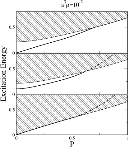
Figure 1: The excitation spectrum according to the RPA, (a), to the HFB theory, (b), and in the Bogoliubov approximation, (c) for $a^{3}\rho=10^{-2}$. In fig 1(a) the solid lines indicate the discrete branch and the continuum threshold, whereas in figs (b) and (c) the lower solid line is the one quasi-particle branch. The dashed line corresponds to the region where the energy of the one quasi-particle branch is greater than the threshold of the two quasi-particle branch. The excitation energy is measured in units of $\hbar^{2}/(2ma^{2})$ and the momenta in units of $\hbar/a$. See text for details.

which corresponds to the relative weight of the one quasi-particle component. Analogously for the two quasi-particle component we can define

$$c_{2}({\bf P})=\sum_{{\bf q}\geq 0}(X_{{\bf q},{\bf P}}^{2}-Y_{{\bf q},{\bf P}}^{2}).$$ (65)

These two relative weights are related through the normalization condition (28) that gives

$$c_{1}({\bf P})+c_{2}({\bf P})=1$$ (66)

Fig. 2(b) and 3(b) show the values of $c_{1}(P)$ and $c_{2}(P)$ as a function of the total momentum $P$ for $a^{3}\rho=10^{-2}$ and $10^{-}3$ respectively. In the long wavelength regime the excitation operator is predominantly a one quasi-particle operator. On the other hand in the short wavelength regime it becomes predominantly a two quasi-particle operator as it approaches asymptotically the continuum threshold. Note that there is a sharp transition between this two regimes, the effect being more pronounced at higher densities. Comparing Figs. 2(a),2(b) and 3(a),3(b), we see that the change from a predominantly one quasi-particle to a predominantly two quasi-particle physical content of the discrete branch of the excitation spectrum and of its corresponding excitation operator occur in the same momentum range.

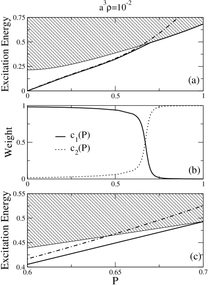
Figure 2: Fig.2(a) shows the RPA discrete excitation energy and continuum threshold (solid lines) and the Bogoliubov one quasi-particle excitation energy (dot-dashed line). In Fig. 2(b) $c_{1}({\bf P})$ (solid line) and $c_{2}({\bf P})$ (dashed line) give , respectively, a measure of the one and two quasi-particle character of the discrete branch, as a function of $P$, for $a^{3}\rho=10^{-2}$, Fig. 2(c) is a zoom of Fig. 2(a) near the transition region. Units as in Fig.1.

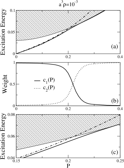
Figure 3: Fig.3(a) shows the RPA discrete excitation energy and continuum threshold (solid lines) and the Bogoliubov one quasi-particle excitation energy (dot-dashed line). In Fig. 3(b) $c_{1}({\bf P})$ (solid line) and $c_{2}({\bf P})$ (dashed line) give , respectively, a measure of the one and two quasi-particle character of the discrete branch, as a function of $P$, for $a^{3}\rho=10^{-3}$, Fig. 3(c) is a zoom of Fig. 2(a) near the transition region. Units as in Fig.1.

VI Conclusion

In this paper we presented a generalization of the HFB theory, cast in terms of well known methods of equations of motion in order to access the excitation spectrum of a condensed many- boson system. The key ingredient for the generalization is the coupling of the one and two quasi-particle components to form the excitation modes. These are determined by solving the appropriate generalized Bogoliubov equations for the relevant amplitudes and excitation energies.

The generalized Bogoliubov equations are shown to have a Goldstone mode at zero transfered momentum, whose structure is related to that generated by the particle number operator. Correspondingly, an examination of the properties of the excitation spectrum reveals a detached gapless excitation branch with phonon-like dispersion at small momenta and a continuum branch starting at the two quasi-particle threshold of the HFB theory. The detached branch has a predominantly one quasi-particle character at small momenta, where it closely approximates the Bogoliubov one quasi-particle spectrum. At high momenta it approaches the continuum threshold and eventually acquires a predominantly two quasi-particle character in what can be seen as an avoided crossing situation, due to the coupling between one and two quasi-particle components included in the calculation. The transition from one to two quasi-particle character is relatively sharp and occurs near the onset of instability of the HFB one quasi-particle spectrum. Differently from the Bogoliubov and HFB approximations the detached phonon-like branch is always stable.

The presence of the continuum branch serves, in particular, to give physical significance to the HFB one quasi-particle energy gap, this being the quantity which sets the appropriate energy scale for the continuum threshold.

The features revealed in this generalized theory are closed linked to the depletion of the condensate caused by the two body interaction effects. They should be particularly relevant, therefore, in cases where such depletion effect become important. This happens for larger condensates densities and/or larger values of the relevant scattering length (implying stronger effective interaction) a situation that may be realized experimentally, for example, by taking advantages of Feshbach resonances.

Appendix A

Appendix A The Grand-Hamiltonian written in normal order

The Grand-Hamiltonian can be written in the following form

$$\hat{h}=\hat{h}_{0}+\hat{h}_{1}+\hat{h}_{2}+\hat{h}_{3}+\hat{h}_{4}$$ (67)

where $\hat{h}_{i}$ corresponds to the normal ordered component with $i$ quasi-particle operators.In turn,we will write each $\hat{h}_{i}$ as :

$$\hat{h}_{i}=\sum_{j=0}^{i}\hat{h}_{i-j,j}$$ (68)

where $i-j$ stands for the number of quasi-particle creation operators and $j$ for the number of annihilation operators. In what follows we will give explicit expressions for all the components appearing in (67)

A.1 i) $\hat{h}_{0}$

$$\hat{h}_{0} = -z_{0}^{2}\mu+\frac{z_{0}^{4}}{2}V(0)+\sum_{\bf k}[e_{k}-\mu+(V(0)+V(k))z_{0}^{2}]v_{\bf k}^{2}$$ (69)

$$-\sum_{\bf k}V(k)z_{0}^{2}u_{\bf k}v_{\bf k}+\frac{1}{2}\sum_{{\bf k_{1}},{\bf k_{2}}}(V(0)+V(|{\bf k_{1}}-{\bf k_{2}}|)v_{\bf k_{1}}^{2}v_{\bf k_{2}}^{2}$$

$$+\frac{1}{2}\sum_{{\bf k_{1}},{\bf k_{2}}}V(|{\bf k_{1}}-{\bf k_{2}}|)u_{\bf k_{1}}v_{\bf k_{1}}u_{\bf k_{2}}v_{\bf k_{2}}$$

A.2 ii) $\hat{h}_{1}$

$$\hat{h}_{1}=h_{10}\eta_{0}^{\dagger}+h_{01}\eta_{0}$$ (70)

where

$$h_{10}=h_{01}=(-\mu+U_{h}+U_{ex}^{nc}(0)+U_{pair}^{nc}(0))z_{0}(x_{0}-y_{0})$$ (71)

From eq.(71) it follows that $\hat{h}_{1}=0$ as a consequence of the equilibrium equation (16).

A.3 iii) $\hat{h}_{2}$

$$\hat{h}_{2} = \sum_{k}h_{11}(\bf k)\eta_{{\bf k}}^{\dagger}\eta_{\bf k}$$ (72)

$$+h_{20}({\bf k})\eta_{\bf k}^{\dagger}\eta_{-\bf k}^{\dagger}+h_{02}({\bf k})\eta_{\bf k}\eta_{-\bf k}$$

where

$$h_{11}({\bf k})=\tilde{e}({\bf k})\cosh 2\sigma_{\bf k}-U_{pair}({\bf k})\sinh 2\sigma_{\bf k}$$ (73)

$$h_{20}({\bf k})=h_{02}({\bf k})=-\tilde{e}({\bf k})\sinh 2\sigma_{\bf k}+U_{pair}({\bf k})\cosh 2\sigma_{\bf k}$$ (74)

From the equilibrium equation (17) we see immediately that the non-diagonal components in equation (72), $h_{20}({\bf k}),h_{02}({\bf k})$ vanish and the coefficient of the diagonal component $h_{11}({\bf k})$ is equal to $\omega_{{\bf k}}$ leading to

$$\hat{h}_{2}=\sum_{k}\omega({\bf k})\eta_{\bf k}^{\dagger}\eta_{\bf k}$$ (75)

A.4 iv) $\hat{h}_{3}$

$\hat{h}_{3}$ can be written as

$$\hat{h}_{3} = \sum_{{\bf k},{\bf k^{\prime}}}\{h_{1,2}({\bf k},{\bf k^{\prime}})\eta_{{\bf k}+{\bf k}}^{\dagger}\eta_{\bf k}\eta_{\bf k^{\prime}}+h_{2,1}({\bf k},{\bf k^{\prime}})\eta_{\bf k^{\prime}}^{\dagger}\eta_{\bf k}^{\dagger}\eta_{{\bf k}+{\bf k^{\prime}}}$$ (76)

$$+h_{3,0}({\bf k},{\bf k^{\prime}})\eta_{{\bf k}+{\bf k^{\prime}}}^{\dagger}\eta_{-{\bf k}}^{\dagger}\eta_{-{\bf k^{\prime}}}^{\dagger}+h_{0,3}({\bf k},{\bf k^{\prime}})\eta_{{\bf k}+{\bf k^{\prime}}}\eta_{-{\bf k}}\eta_{-{\bf k^{\prime}}}\}$$

where the $h_{i,k}$ coefficients are given by

$$h_{1,2}({\bf k},{\bf k^{\prime}}) = h_{2,1}({\bf k},{\bf k^{\prime}})=\frac{z_{0}}{2}\left\{[u_{{\bf k}+{\bf k^{\prime}}}u_{\bf k^{\prime}}+v_{{\bf k}+\bf{k^{\prime}}}v_{\bf k^{\prime}}][u_{\bf k}-v_{\bf k}]V(k)\right.$$ (77)

$$\left.+[u_{{\bf k}+{\bf k^{\prime}}}u_{\bf k}+v_{{\bf k}+\bf{k^{\prime}}}v_{\bf k}][u_{\bf k^{\prime}}-v_{\bf k^{\prime}}]V(k^{\prime})\right.$$

$$\left.-[u_{{\bf k}+{\bf k}^{\prime}}-v_{{\bf k}+{\bf k}^{\prime}}][u_{\bf k}v_{\bf k^{\prime}}+v_{\bf k}u_{\bf k^{\prime}}]V(|{\bf k}+{\bf k^{\prime}}|)\right\}$$

$$h_{3,0}({\bf k},{\bf k^{\prime}}) = h_{0,3}({\bf k},{\bf k^{\prime}})=\frac{z_{0}}{2}\left\{[u_{{\bf k}+{\bf k^{\prime}}}v_{\bf k}v_{\bf k^{\prime}}-v_{{\bf k}+{\bf k^{\prime}}}u_{\bf k}u_{\bf k^{\prime}}][V(k)+V(k^{\prime})]\right\}.$$

Note that all the coefficients obey the symmetry propriety $h_{i,j}({\bf k},{\bf k^{\prime}})=h_{i,j}(-{\bf k},-{\bf k^{\prime}})=h_{i,j}({\bf k^{\prime}},{\bf k})$.

A.5 v) $\hat{h}_{4}$

Analogously to the previous case we can write $\hat{h}_{4}$ as

$$\hat{h}_{4} = \sum_{{\bf k_{1}},{\bf k_{2}},{\bf q}}h_{1,3}({\bf k_{1}},{\bf k_{2}},{\bf q})\eta_{{\bf k_{2}}-{\bf q}}^{\dagger}\eta_{-{\bf k_{1}}-{\bf q}}\eta_{{\bf k_{1}}}\eta_{\bf k_{2}}$$ (79)

$$+h_{3,1}({\bf k_{1}},{\bf k_{2}},{\bf q})\eta_{{\bf k_{1}}}^{\dagger}\eta_{{\bf k_{2}}}^{\dagger}\eta_{-{\bf k_{1}}-{\bf q}}^{\dagger}\eta_{{\bf k_{2}}-{\bf q}}$$

$$+h_{4,0}({\bf k_{1}},{\bf k_{2}},{\bf q})\eta_{{\bf k_{1}}+{\bf q}}^{\dagger}\eta_{{\bf k_{2}}-{\bf q}}^{\dagger}\eta_{-{\bf k_{1}}}^{\dagger}\eta_{-{\bf k_{2}}}^{\dagger}$$

$$+h_{0,4}({\bf k_{1}},{\bf k_{2}},{\bf q})\eta_{{\bf k_{1}}+{\bf q}}\eta_{{\bf k_{2}}-{\bf q}}\eta_{-{\bf k_{1}}}\eta_{-{\bf k_{2}}}$$

$$+h_{2,2}({\bf k_{1}},{\bf k_{2}},{\bf q})\eta_{{\bf k_{1}}+{\bf q}}^{\dagger}\eta_{{\bf k_{2}}-{\bf q}}^{\dagger}\eta_{{\bf k_{1}}}\eta_{\bf k_{2}}$$

where the coefficients are given by

$$h_{3,1}({\bf k_{1}},{\bf k_{2}},{\bf q})=h_{1,3}({\bf k_{1}},{\bf k_{2}},{\bf q})=-[u_{{\bf k_{2}}-{\bf q}}v_{{\bf k_{1}}+{\bf q}}u_{\bf k_{1}}u_{\bf k_{2}}+$$

$$v_{{\bf k_{2}}-{\bf q}}u_{{\bf k_{1}}+{\bf q}}v_{\bf k_{1}}v_{\bf k_{2}}]V(q)$$ (80)

$$\hat{h}_{4,0}({\bf k_{1}},{\bf k_{2}},{\bf q})=\hat{h}_{0,4}({\bf k_{1}},{\bf k_{2}},{\bf q})=\frac{1}{2}u_{{\bf k_{1}}+{\bf q}}u_{{\bf k_{2}}-{\bf q}}v_{\bf k_{1}}v_{\bf k_{2}}V(q)$$ (81)

$$\hat{h}_{2,2}({\bf k_{1}},{\bf k_{2}},{\bf q})=\frac{1}{2}\{[u_{{\bf k_{1}}+{\bf q}}u_{\bf k_{1}}+v_{{\bf k_{1}}+{\bf q}}v_{\bf k_{1}}][u_{{\bf k_{2}}-{\bf q}}u_{\bf k_{2}}+v_{{\bf k_{2}}-{\bf q}}v_{\bf k_{2}}]V(q)$$

$$+[u_{{\bf k_{2}}-{\bf q}}u_{\bf k_{1}}v_{{\bf k_{1}}+{\bf q}}v_{\bf k_{2}}+u_{{\bf k_{1}}+{\bf q}}u_{{\bf k_{2}}}v_{{\bf k_{2}}-{\bf q}}v_{\bf k_{1}}]V(|{\bf k_{1}}+{\bf k_{2}}|)\}$$ (82)

These coefficients,except $h_{3,1}$ and $h_{1,3}$ obey the symmetry property

$$h_{i,j}({\bf k_{1}},{\bf k_{2}},{\bf q})=h_{i,j}({\bf k_{2}},{\bf k_{1}},-{\bf q})=h_{i,j}(-{\bf k_{1}},-{\bf k_{2}},-{\bf q})$$ (83)

Appendix B

Appendix B RPA Matrices

In this appendix we evaluate the elements of the matrices $\cal A$ and $\cal B$. The key property that we will use to calculate the average value of the symmetrized double commutators is that $|\Phi\rangle$ is the quasi-particle vacuum. In order to work with more compact expressions we introduce the following quantities

$$C_{0}({\bf k}) = u_{\bf k}-v_{\bf k}$$ (84)

$$C_{1}({\bf k},{\bf k^{\prime}}) = C_{1}({\bf k}^{\prime},{\bf k})=C_{1}(-{\bf k},-{\bf k^{\prime}})=u_{\bf k}u_{\bf k^{\prime}}+v_{\bf k}v_{\bf k^{\prime}}$$ (85)

$$C_{2}({\bf k},{\bf k^{\prime}}) = C_{2}({\bf k}^{\prime},{\bf k})=C_{2}(-{\bf k},-{\bf k^{\prime}})=u_{\bf k}v_{\bf k^{\prime}}+v_{\bf k}u_{\bf k^{\prime}}.$$ (86)

where (85) and (86) are usually called coherence factors and are well known in the study of Bose systems 9 .

B.1 The matrix $\cal A$

${\cal A}^{11}({\bf P})$ is given by,

$${\cal A}^{11}({\bf P})=\langle\Phi|[\eta_{\bf P},H,\eta_{\bf P}^{\dagger}]|\Phi\rangle.$$ (87)

From the property that $|\Phi\rangle$ is the quasi-particle vacuum it follows immediately that only $\hat{h}_{2}$ contributes to this matrix element, with the result

$${\cal A}^{11}({\bf P})=\omega({\bf P}).$$ (88)

The elements of the $1\times npair$ matrix ${\cal A}^{12}$ are given by

$${\cal A}^{12}({\bf q};{\bf P})=\langle\Phi|[\eta_{\bf P},H,\frac{\eta_{{\bf q}+{\bf P}/2}^{\dagger}\eta_{-{\bf q}+{\bf P}/2}^{\dagger}}{\sqrt{1+\delta_{{\bf q},0}}}]|\Phi\rangle$$ (89)

The only contribution to this matrix element comes from $\hat{h}_{3}$ through the term $\hat{h}_{12}$ , giving

$${\cal A}^{12}({\bf q};{\bf P}) = -2\frac{h_{1,2}({\bf q}+{\bf P}/2,-{\bf q}+{\bf P}/2)}{\sqrt{1+\delta_{{\bf q},0}}}.$$ (90)

Using the expression for $h_{12}$ term show in Eq.(77) we can write (90) in terms of the coherence factors (85), (86) obtaining

$${\cal A}^{12}({\bf q};{\bf P})=\frac{1}{\sqrt{1+\delta_{{\bf q},0}}}\{C_{0}(+)C_{1}({\bf P},-)V(+)+C_{0}(-)C_{1}({\bf P},+)V(-)$$

$$-C_{0}(P)C_{2}(+,-)V(P)\}$$ (91)

where we used the notation $\pm=\pm{\bf q}+{\bf P}/2$ and $\pm^{\prime}=\pm{\bf q}^{\prime}+{\bf P}/2$. The elements of the $npairs\times 1$ matrix ${\cal A}^{21}$ is the hermitian conjugate of the matrix ${\cal A}^{12}$. The elements of $npairs\times npairs$ matrix ${\cal A}^{22}({\bf q^{\prime}},{\bf q};{\bf P})$ are given by

$${\cal A}^{22}({\bf q^{\prime}},{\bf q};{\bf P})=\langle\Phi|[\frac{\eta_{{\bf q^{\prime}}+{\bf P}/2}\eta_{-{\bf q^{\prime}}+{\bf P}/2}}{\sqrt{1+\delta_{{\bf q^{\prime}},0}}},H,\frac{\eta_{{\bf q}+{\bf P}/2}^{\dagger}\eta_{-{\bf q}+{\bf P}/2}^{\dagger}}{\sqrt{1+\delta_{{\bf q},0}}}]|\Phi\rangle,$$ (92)

Both $\hat{h}_{2}$, through the term $\hat{h}_{1,1}$, and $\hat{h}_{4}$ through the term $\hat{h}_{2,2}$ contribute to this matrix element, leading to

$${\cal A}^{22}({\bf q^{\prime}},{\bf q};{\bf P})=[\omega(-{\bf q}+{\bf P}/2)+\omega({\bf q}+{\bf P}/2)]\delta_{{\bf q},{\bf q}^{\prime}}+\frac{1}{\sqrt{(1+\delta_{{\bf q},0})(1+\delta_{{\bf q}^{\prime},0})}}\{$$

$$h_{2,2}({\bf q}+{\bf P}/2,-{\bf q}+{\bf P}/2,{\bf q}^{\prime}-{\bf q})+h_{2,2}({\bf q}^{\prime}+{\bf P}/2,-{\bf q}^{\prime}+{\bf P}/2,{\bf q}-{\bf q}^{\prime})+$$

$$h_{2,2}(-{\bf q}+{\bf P}/2,{\bf q}+{\bf P}/2,{\bf q}^{\prime}+{\bf q})+h_{2,2}(-{\bf q}^{\prime}+{\bf P}/2,{\bf q}^{\prime}+{\bf P}/2,{\bf q}+{\bf q}^{\prime})\}.$$ (93)

Using the expression for $h_{2,2}$ calculated in the previous appendix we get

$${\cal A}^{22}({\bf q^{\prime}},{\bf q};{\bf P})=[\omega(-)+\omega(+)]\delta_{{\bf q},{\bf q}^{\prime}}+\frac{1}{\sqrt{(1+\delta_{{\bf q},0})(1+\delta_{{\bf q}^{\prime},0})}}\{$$

$$C_{2}(+^{\prime},-^{\prime})C_{2}(+,-)V(P)+C_{1}(+,+^{\prime})C_{1}(-,-^{\prime})V(|{\bf q}-{\bf q}^{\prime}|)+$$

$$C_{1}(+^{\prime},-)C_{1}(+,-^{\prime})V(|{\bf q}+{\bf q}^{\prime}|)\}$$ (94)

B.2 The matrix $\cal B$

For the matrix B we start with $B^{11}$

$${\cal B}^{11}({\bf P})=\langle\Phi|[\eta_{\bf P},H,\eta_{\bf-P}]|\Phi\rangle,$$ (95)

By inspection, we see that there are no terms in the Hamiltonian that contributes to this matrix element, hence

$${\cal B}^{11}({\bf P})=0.$$ (96)

Next we consider the matrix elements of ${\cal B}^{12}$ given by

$${\cal B}^{12}({\bf q};{\bf P})=\langle\Phi|[\eta_{\bf P},H,\frac{\eta_{-{\bf q}-{\bf P}/2}\eta_{{\bf q}-{\bf P}/2}}{\sqrt{1+\delta_{{\bf q},0}}}]|\Phi\rangle,$$ (97)

In this case the only contribution comes from $\hat{h}_{3}$ through the term $\hat{h}_{3,0}$

$${\cal B}^{12}({\bf q};{\bf P}) = -\frac{2}{\sqrt{1+\delta_{{\bf q},0}}}[h_{3,0}({\bf q}+{\bf P}/2,-{\bf q}+{\bf P}/2)+$$ (98)

$$h_{3,0}(-{\bf q}+{\bf P}/2,-{\bf P})+h_{3,0}({\bf q}+{\bf P}/2,-{\bf P})]$$

which can be written in terms of the coherence factors as

$${\cal B}^{12}({\bf q};{\bf P})=-\frac{1}{\sqrt{1+\delta_{{\bf q},0}}}\{C_{0}(+)C_{2}({\bf P},-)V(+)$$

$$C_{0}(-)C_{2}({\bf P},+)V(-)+C_{0}(P)C_{2}(+,-)V(P)]\}$$ (99)

The matrix ${\cal B}^{12}$ is the transpose of ${\cal B}^{12}$.

For $B^{22}({\bf q^{\prime}},{\bf q};{\bf P})$ we have

$$B^{22}({\bf q^{\prime}},{\bf q};{\bf P})=\langle\Phi|[\frac{\eta_{{\bf q^{\prime}}+{\bf P}/2}\eta_{-{\bf q^{\prime}}+{\bf P}/2}}{\sqrt{1+\delta_{{\bf q^{\prime}},0}}},H,\frac{\eta_{{\bf q}-{\bf P}/2}\eta_{-{\bf q}-{\bf P}/2}}{\sqrt{1+\delta_{{\bf q},0}}}|\Phi\rangle,$$ (100)

The only non vanishing contribution to this matrix element comes from $\hat{h}_{4}$ through the term $\hat{h}_{4,0}$, giving:

$$B^{22}({\bf q^{\prime}},{\bf q};{\bf P})=-h_{0,4}(-{\bf q}+{\bf P}/2,-{\bf q}^{\prime}-{\bf P}/2,{\bf q}-{\bf q^{\prime}})$$

$$-h_{0,4}({\bf q}+{\bf P}/2,-{\bf q^{\prime}}-{\bf P}/2,-{\bf q}^{\prime}-{\bf q})$$

$$-h_{0,4}(-{\bf q}+{\bf P}/2,{\bf q}+{\bf P}/2,-{\bf q}^{\prime}+{\bf q})$$

$$-h_{0,4}({\bf q}+{\bf P}/2,-{\bf q}+{\bf P}/2,-{\bf q}-{\bf q}^{\prime})$$

$$-h_{0,4}(-{\bf q}+{\bf P}/2,{\bf q^{\prime}}-{\bf P}/2,{\bf q}^{\prime}+{\bf q})$$

$$-h_{0,4}({\bf q}+{\bf P}/2,{\bf q}^{\prime}-{\bf P}/2,{\bf q}^{\prime}-{\bf q})$$

$$-h_{0,4}(-{\bf q}+{\bf P}/2,{\bf q}+{\bf P}/2,{\bf q}+{\bf q^{\prime}})$$

$$-h_{0,4}({\bf q}+{\bf P}/2,-{\bf q}+{\bf P}/2,{\bf q}^{\prime}-{\bf q})$$

$$-h_{0,4}({\bf q}^{\prime}-{\bf P}/2,-{\bf q}+{\bf P}/2,{\bf P})-h_{0,4}({\bf q}^{\prime}-{\bf P}/2,{\bf q}+{\bf P}/2,{\bf P})$$

$$-h_{0,4}(-{\bf q}^{\prime}-{\bf P}/2,-{\bf q}+{\bf P}/2,{\bf P})-h_{0,4}(-{\bf q}^{\prime}-{\bf P}/2,{\bf q}+{\bf P}/2,{\bf P})$$

$$+q\rightleftharpoons q^{\prime},P\rightarrow-P$$ (101)

which can be written, in terms of the coherence factors as

$$B^{22}({\bf q^{\prime}},{\bf q};{\bf P})=-\frac{1}{\sqrt{(1+\delta_{{\bf q},0})(1+\delta_{{\bf q}^{\prime},0})}}\{C_{2}[+,+^{\prime}]C_{2}[-,-^{\prime}][V(|{\bf q}+{\bf q}^{\prime}|)$$

$$+V(|{\bf q}-{\bf q}^{\prime}|)]+C_{2}[+,-]C_{2}[+^{\prime},-^{\prime}]V(P)\}$$ (102)

Appendix C Acknoledgements

This work was supported by FAPESP under the contract number 00/00649-9. P.T. and M.O.C.P. are supported by FAPESP. EJVP is partially supported by CNPq. The authors would like to thank Dr. Eddy Timmermnas for his critical reading of the manuscript.

References

• (1) K.B. Davis et al Phys. Rev. Lett. 75, 3969 (1995), M.H. Anderson et al. Science 296, 198 (1995) and C.C. Bradley et al Phys. Rev. Lett. 75, 1687 (1995)
• (2) F. Dalfovo, S. Giorgini, L.P. Pitaevskii and S. Stringari, Rev. Mod. Phys. 71, 463 (1999).
• (3) P.A. Ruprecht, M. Edwards, K. Burnett and C.W. Clark Phys. Rev. A 54, 4178 (1996).
• (4) M. Edwards,P.A. Ruprecht, K. Burnett, R. J. Dodd and C.W. Clark Phys. Rev. Lett. 77, 1671 (1996).
• (5) D.A. Hutchinson, W. Zaremba and A. Griffin Phys. Rev. Lett 78, 1842 (1997)
• (6) A. Griffin Phys. Rev B 53, 9341 (1996)
• (7) S.L. Cornish, N.R. Claussen, J.L. Roberts, E.A. Cornell and C.E. Wieman Phys. Rev. Lett. 85, 1795 (2000).
• (8) N.M. Hugenholtz and D. Pines Phys Rev. 116, 489(1959).
• (9) A. Griffin, Excitations in a Bose-Condensed Liquid, (Cambridge University Press, 1993).
• (10) F. Takano, Phys. Rev 123, 699 (1961).
• (11) D.A.W. Hutchinson et al, J. Phys. B 33, 3825 (2000).
• (12) A. K. Kerman, P. Tommasini, Ann. Phys. 260, 250 (1997).
• (13) D.J. Rowe, Rev. Mod. Phys. 40, 153 (1968).
• (14) J. Dukelsky and P. Schuck, Nucl. Phys. A 628, 17 (1998).
• (15) Z. Aouissat, G. Chanfray, P. Schuck e J. Wambach, Nucl. Phys. A 603, 458 (1996).
• (16) A.L. Fetter and J.D. Walecka, Quantum theory of many particle systems (McGraw-Hill, 1971).
• (17) W.A.B. Evans and Y. Imry, Nuovo Cimento B 63, 155 (1969).
• (18) J.P. Blaizot and G. Ripka Quantum theroy of finite systems (MIT press, 1986)
• (19) S. Giorgini, J.Boronat, and J. Casulleras, Phys. Rev. A 60, 5129 (1999)
• (20) S. Fantoni, T.M. Nguyen, A. Sarsa and S.R. Shenoy Phys. Rev A 66, 033604 (2002).
• (21) P. Noziéres, D. Pines The Theory of Quantum Liquids (Perseu Books Publishing, L.L.C., 1999)