One and Two-Electron Spectral Function Expressions in the Vicinity of the Upper-Hubbard Bands Lower Limit

Abstract

In this paper we derive general expressions for few-electron spectral functions of the one-dimensional Hubbard model for values of the excitation energy in the vicinity of the $M^{th}$ upper-Hubbard band lower limit. Here $M=1,2,...$ is the rotated-electron double occupation, which vanishes for the ground state and is a good quantum number for all values of the on-site Coulomb repulsion $U$. Our studies rely on a combination of symmetries of the model with a recent finite-energy holon and spinon description of the quantum problem. We apply our general scheme to the one-electron addition spectral function, dynamical structure factor, and spin singlet Cooper pair addition spectral function. Our results provide physically interesting information about the finite-energy spectral properties of the many-electron one-dimensional quantum liquid.

1 INTRODUCTION

Recent experimental studies of quasi-one-dimensional (1D) materials observed unusual finite-energy/frequency spectral properties, which are far from being well understood [1, 2, 3, 4, 5]. Several of these experimental studies reveal the occurrence of charge-spin separation in terms of independent holon and spinon excitation modes [2, 4, 5, 6, 7, 8, 9, 10]. For values of the excitation energy larger than the transfer integrals associated with electron hopping between the chains, the 1D Hubbard model [11] is expected to provide a good description of the physics of these materials [4, 5]. Unfortunately, an accurate determination of the spectral properties for finite values of the excitation energy and of the Coulomb repulsion is until now still lacking. Most accurate results correspond to the limit of infinite on-site Coulomb repulsion [12] where the Bethe-ansatz [11] wave function is easier to handle, yet the solution of the problem remains complex in this limit.

In this paper we combine the holon, spinon, and pseudoparticle accurate description recently introduced and studied in Refs. [6, 7] and the pseudofermion representation very recently introduced in Ref. [8] with symmetries of the 1D Hubbard model to derive general expressions for few-electron spectral functions in the vicinity of the lower limit of the upper Hubbard bands. For finite values of the excitation energy and on-site repulsion $U$ there are not many previous studies of few-electron spectral function weight distributions. The interesting studies of the one-electron spectral functions presented in Ref. [12] refer to the limit of infinite $U$. There are numerical studies of these functions for $U\approx 4t$ [13]. Moreover, the weight distribution of the real part of the frequency dependent optical conductivity in the vicinity of the optical pseudogap was previously studied in Refs. [14, 15]. The very recent results presented in Ref. [10] refer to the one-electron spectral-function weight-distribution in the vicinity of singular branch lines. Some of these lines cross the upper-Hubbard band lower-limit points considered in this paper. However, our results are complementary of those presented in Ref. [10], which were obtained by use of the method of Ref. [16]. Indeed, our weight-distribution expressions are valid when one approaches these points along all finite-weight directions except those corresponding to the above-mention singular branch lines. The values of the critical exponents which control the weight distribution are different for these lines and for all the remaining directions of the ($k,\,\omega$)-plane considered here.

We evaluate expressions for the critical exponents that control the weight distribution of few-electron spectral functions for excitation energies corresponding to the vicinity of the $M^{th}$ upper Hubbard band lower-limit points. (The method used in this paper is different from that of Ref. [16], which was used in Ref. [10] in the study of the weight distribution in the vicinity of the singular branch lines.) Our studies rely on a symmetry which is specific for the model when defined in the reduced Hilbert subspace associated with the ($k,\,\omega$)-plane region in the vicinity of the above lower-limit points. Few-electron spectral functions can include several upper Hubbard bands, the $M^{th}$ band being spanned by excited states of rotated electron double occupation $M>0$. The lower Hubbard band corresponds to the spectral-weight distribution generated by excited states of rotated-electron double occupation $M=0$. For one-electron and two-electron spectral functions only the first few upper bands have a significant amount of spectral weight [16]. Although our general expressions refer to the lower-limit points of all upper Hubbard bands, we apply our method only to the study of weight distributions corresponding to upper bands with a significant amount of spectral weight. For the one-electron addition spectral function and dynamical structure factor (and the spin singlet Cooper pair addition spectral function) only the $M=1$ first Hubbard band has (and both the $M=1$ first and $M=2$ second upper Hubbard bands have) a significant amount of weight.

Our motivation in studying the finite-energy one-electron spectral function is that our method provides the exponents of the singular spectral features beyond the branch lines considered in Ref. [10]. The latter lines are observed in quasi-1D materials [9, 10]. Thus, the study of other finite-energy singular spectral features is of interest for the further understanding of the unusual spectral properties observed in these materials. Both for the dynamical structure factor and other spectral functions we do not consider the low-energy features because those can be investigated by standard two-component conformal-field theory. Our aim in studying the Cooper-pair spectral function is to clarify whether there are singular spectral features at the upper-Hubbard bands lower limit. Indeed, in the limit of small on-site repulsion and for electronic densities very close to one, such singular features would appear at low energy and could lead to a superconductivity instability in a system of weakly coupled Hubbard chains, as further discussed in later sections.

The paper is organized as follows: In Sec. II we summarize the 1D Hubbard model. In Sec. III we introduce the holon-spinon Hamiltonian and study the 1D Hubbard model spectrum in the vicinity of the lower limit of the upper Hubbard bands. In Sec. IV we use the holon and spinon conservation laws and other symmetries of the model in the evaluation of general expressions for few-electron spectral functions. Moreover, we apply our method to the study of the one-electron addition spectral function, dynamical structure factor, and singlet Cooper pair addition spectral function. Finally, Sec. V contains the concluding remarks.

2 THE 1D HUBBARD MODEL

In a chemical potential $\mu$ and magnetic field $H$ the 1D Hubbard Hamiltonian can be written as,

$$\hat{H}={\hat{H}}_{SO(4)}+\sum_{\alpha=c,\,s}\mu_{\alpha}\,{\hat{S}}^{\alpha}_{z}\,;$$

$${\hat{H}}_{SO(4)}=-t\sum_{j=1}^{N_{a}}\sum_{\sigma=\uparrow,\downarrow}[c_{j,\,\sigma}^{{\dagger}}\,c_{j+1,\,\sigma}+c^{{\dagger}}_{j+1,\,\sigma}\,c_{j,\,\sigma}]+U\,\sum_{j=1}^{N_{a}}[\hat{n}_{j,\,\uparrow}-1/2]\,[\hat{n}_{j,\,\downarrow}-1/2]\,,$$

where $c_{j,\,\sigma}^{\dagger}$ and $c_{j,\,\sigma}$ are the spin $\sigma$ electron creation and annihilation operators at site $j$, respectively. The operator $\hat{n}_{j,\,\sigma}=c_{j,\,\sigma}^{\dagger}\,c_{j,\,\sigma}$ counts the number of spin $\sigma$ electrons at real-space lattice site $j=1,...,N_{a}$. The number of lattice sites $N_{a}$ is even and large and $N_{a}/2$ is odd. We consider periodic boundary conditions. Moreover, $\mu_{c}=2\mu$, $\mu_{s}=2\mu_{0}H$, $\mu_{0}$ is the Bohr magneton, and ${\hat{S}}^{c}_{z}=-(1/2)[N_{a}-\hat{N}]$ and ${\hat{S}}^{s}_{z}=-(1/2)[{\hat{N}}_{\uparrow}-{\hat{N}}_{\downarrow}]$ are the diagonal generators of the $\eta$-spin and spin $SU(2)$ algebras [17], respectively. The operators ${\hat{N}}=\sum_{\sigma}\hat{N}_{\sigma}$ and ${\hat{N}}_{\sigma}=\sum_{j}\hat{n}_{j,\,\sigma}$ count the number of electrons and spin $\sigma$ electrons, respectively. The Hamiltonian $\hat{H}_{SO(4)}$ defined in Eq. (2) commutes with the six generators of the $\eta$-spin and spin algebras [17]. The Bethe-ansatz solvability of the 1D Hubbard model is restricted to the Hilbert subspace spanned by the lowest-weight states (LWSs) of the $\eta$ spin and spin algebras, i.e. such that $S^{\alpha}=-S^{\alpha}_{z}$ [6] for $\alpha=c$ and $\alpha=s$, respectively. Here $S_{c}$ (and $S_{s}$) denotes the $\eta$-spin (and spin) value. The momentum operator reads,

$$\hat{P}=\sum_{\sigma=\uparrow,\,\downarrow}\sum_{k}\,\hat{N}_{\sigma}(k)\,k\,,$$ (2)

where the spin $\sigma$ momentum distribution operator is given by $\hat{N}_{\sigma}(k)=c_{k,\,\sigma}^{\dagger}\,c_{k,\,\sigma}$ and the operator $c_{k,\,\sigma}^{\dagger}$ (and $c_{k,\,\sigma}$) creates (and annihilates) a spin $\sigma$ electron at momentum $k$. The momentum operator (2) commutes with the Hamiltonians of Eq. (2).

There are $N_{\uparrow}$ spin-up electrons and $N_{\downarrow}$ spin-down electrons in the chain of $N_{a}$ sites, lattice constant $a$, and length $L=[N_{a}\,a]$ associated with the model (2). Throughout this paper we use units of Planck constant one and of lattice spacing $a=1$ and denote the electronic charge by $-e$. The Fermi momenta read $k_{F\sigma}=\pi n_{\sigma}$ and $k_{F}=\pm[k_{F\uparrow}+k_{F\downarrow}]/2=\pi n/2$, where $n_{\sigma}=N_{\sigma}/N_{a}$ and $n=N/N_{a}$. The electronic density can be written as $n=n_{\uparrow}+n_{\downarrow}$ and the spin density is given by $m=n_{\uparrow}-n_{\downarrow}$. In general we consider electronic densities $n$ and spin densities $m$ in the domains $0\leq n\leq 1$ and $0\leq m\leq n$, respectively. Our general correlation-function expressions are derived for the metallic phase of electronic densities $0<n<1$ and spin densities $0<m<n$. However, taking the limit $n\rightarrow 1$ in some of these expressions leads to correct expressions for the $n=1$ Mott-Hubbard insulator phase. Also the $m=0$ spectral function expressions can in general be obtained by taking the limit $m\rightarrow 0$ in our general expressions. In our applications to the study of specific spectral functions we consider such $m=0$ expressions only.

The concept of rotated electron [6, 7, 8] is associated with a unitary transformation introduced in Ref. [18]. For such rotated electrons, double occupation is a good quantum number for all values of the on-site Coulombian repulsion $U$. The electrons that occur in the 1D Hubbard model (2) are defined by $c_{j,\,\sigma}^{{\dagger}}$, while the rotated electron operator ${\tilde{c}}_{j,\,\sigma}^{{\dagger}}$ is given by, ${\tilde{c}}_{j,\,\sigma}^{{\dagger}}={\hat{V}}^{{\dagger}}(U/t)\,c_{j,\,\sigma}^{{\dagger}}\,{\hat{V}}(U/t)$, where ${\hat{V}}(U/t)$ is the electron - rotated-electron unitary operator defined by Eqs. (10)-(12) of Ref. [8]. As a result of the Hilbert-space electron - rotated-electron unitary rotation, all energy eigenstates of the model are described in terms of occupancy configurations of $s_{c}=1/2$ and $\sigma_{c}=\pm 1/2$ holons, $s_{s}=1/2$ and $\sigma_{s}=\pm 1/2$ spinons, and $c$ pseudoparticles [6]. Here we denoted the $\eta$-spin and spin projections of the quantum objects by $\sigma_{c}$ and $\sigma_{s}$, respectively, whereas their $\eta$-spin and spin values are denoted by $s_{c}$ and $s_{s}$, respectively. In this paper we call the holons and spinons according to their values of $\sigma_{c}=\pm 1/2$ and $\sigma_{s}=\pm 1/2$, respectively. We denote by $M_{\alpha,\,\pm 1/2}$ the number of $\pm 1/2$ holons ($\alpha=c$) or $\pm 1/2$ spinons ($\alpha=s$). The value of the number of rotated-electron doubly occupied and unoccupied sites (and spin-down and spin-up rotated-electron singly occupied sites) equals that of the holon numbers $M_{c,\,-1/2}$ and $M_{c,\,+1/2}$ (and spinon numbers $M_{s,\,-1/2}$ and $M_{s,\,+1/2}$), respectively. Thus, rotated-electron double occupation $M$ is such that $M=M_{c,\,-1/2}$. Moreover, $M_{\alpha}=M_{\alpha,\,+1/2}+M_{\alpha,\,-1/2}$ and $N_{c}=M_{s}$, where $N_{c}$ is the number of $c$ pseudoparticles. The $\pm 1/2$ holons and $c$ pseudoparticles carry charge $\pm 2e$ and $-e$, respectively, whereas the spinons have no charge degrees of freedom. The $c\nu$ pseudoparticles (and $s\nu$ pseudoparticles) associated with Takahasi’s charge (and spin) ideal string excitations of length $\nu$ [11, 6] are $\eta$-spin singlet $2\nu$-holon (and spin singlet $2\nu$-spinon) composite quantum objects [6, 7, 8]. The $\pm 1/2$ holons (and $\pm 1/2$ spinons) which are not part of such $2\nu$-holon composite $c\nu$ pseudoparticles (and $2\nu$-spinon composite $s\nu$ pseudoparticles) are called $\pm 1/2$ Yang holons (and $\pm 1/2$ HL spinons) [6]. In the designations HL spinon and Yang holon, HL stands for Heilmann and Lieb and Yang refers to C. N. Yang, respectively, who are the authors of the papers of Ref. [17]. We denote by $N_{\alpha\nu}$ the number of composite $\alpha\nu$ pseudoparticles belonging to branches $\alpha=c,\,s$ and $\nu=1,2,...$. We call $L_{\alpha,\,\pm 1/2}$ the number of $\pm 1/2$ Yang holons ($\alpha=c$) or $\pm 1/2$ HL spinons ($\alpha=s$). Note that $M_{\alpha,\,\pm 1/2}=L_{\alpha,\,\pm 1/2}+\sum_{\nu=1}^{\infty}\nu\,N_{\alpha\nu}$.

Below we are mostly interested in excited states without HL spinons and $s\nu$ pseudoparticles such that $\nu>1$. Therefore, for simplicity often we replace the pseudoparticle branch index $s1$ by $s$. Thus, throughout this paper the notations $s1$ and $s$ are equivalent. For the subspaces spanned by the ground state and excited states generated from it by a finite number of pseudoparticle and/or Yang holon processes, the $c$, $s$, and $c1$ pseudoparticles carry band momentum $q$ such that $|\,q|\leq q_{c}^{0}=\pi$, $|\,q|\leq q_{s}^{0}=k_{F}$, and $|\,q|\leq q_{c1}^{0}=[\pi-2k_{F}]$, respectively. This refers to electronic densities $0<n<1$ and spin density $m=0$. For these densities the ground state is such that there are no $-1/2$ Yang holons, the $c1$ and $s$ pseudoparticle bands are empty and filled, respectively, and the $c$ pseudoparticles occupy $0\leq|\,q|\leq q_{Fc}^{0}=2k_{F}$ and thus leave $2k_{F}<|\,q|\leq\pi$ empty [6, 7]. Following the notation of Ref. [7], we call an electron ensemble space a Hilbert subspace spanned by all states with fixed values for the $N_{\uparrow}$ and $N_{\downarrow}$ electron numbers. Furthermore, we call a CPHS ensemble space, where CPHS stands for $c$ pseudoparticle, $-1/2$ holon, and $-1/2$ spinon, a Hilbert subspace spanned by all states with fixed values for the numbers $N_{c}$, $M_{c,\,-1/2}$, and $M_{s,\,-1/2}$. A CPHS ensemble subspace is a Hilbert subspace spanned by all states with fixed values for the numbers $N_{c}$, $L_{c,\,-1/2}$, and $L_{s,\,-1/2}$ and for the sets of numbers $\{N_{c\nu}\}$ and $\{N_{s\nu}\}$ corresponding to $\nu=1,2,...$ branches. We note that one does not need to provide the values of $M_{c,\,+1/2}$ and $M_{s,\,+1/2}$ in order to specify a CPHS ensemble space, since these numbers are not independent [7]. Also the numbers $L_{c,\,+1/2}$ and $L_{s,\,+1/2}$ are not independent and one does not need to provide these values in order to specify a CPHS ensemble subspace.

Finally, let us introduce the useful quantum number $\iota=sgn(q)1=\pm 1$ which refers to the number of right pseudoparticle movers ($\iota=+1$) and left pseudoparticle movers ($\iota=-1$). The numbers $N_{c,\,\iota}$ of $c$ pseudoparticles and $N_{\alpha\nu,\,\iota}$ of $\alpha\nu$ pseudoparticles of $\iota$ character are good quantum numbers. We thus introduce the $c$ pseudoparticle and $\alpha\nu$ pseudoparticle current numbers,

$$J_{c}={1\over 2}\sum_{\iota=\pm 1}(\iota)\,N_{c,\,\iota}\,;\hskip 14.22636ptJ_{\alpha\nu}={1\over 2}\sum_{\iota=\pm 1}(\iota)\,N_{\alpha\nu,\,\iota}\,.$$ (3)

The numbers $N_{c,\,\iota}$ and $N_{\alpha\nu,\,\iota}$ can be expressed as $N_{c,\,\iota}=N_{c}/2+\iota\,J_{c}$ and $N_{\alpha\nu,\,\iota}=N_{\alpha\nu}/2+\iota\,J_{\alpha\nu}$.

Each CPHS ensemble Hilbert subspace characterized by fixed values for the sets of numbers $N_{c}$, $\{N_{\alpha\nu}\}$ such that $\alpha=c,s$ and $\nu=1,2,3,...$, and $\{L_{\alpha,\,-1/2}\}$ such that $\alpha=c,s$ contains different subspaces with different values for the sets of current numbers $J_{c}$ and $\{J_{\alpha\nu}\}$ such that $\alpha=c,s$ and $\nu=1,2,...$. According to the notation of Ref. [8], we call these subspaces J-CPHS ensemble subspaces.

3 THE HOLON-SPINON HAMILTONIAN AND THE UPPER HUBBARD BANDS LOWER LIMIT SPECTRUM

The correlation function expressions are determined by transitions from the ground state to excited states. Let us consider that the initial ground state belongs to a canonical ensemble space associated with densities such that $0<n<1$ and $0<m<n$. Often we consider such ground states. In the application of our results to the evaluation of specific spectral function expressions we are mostly interested in $m=0$ initial ground states. Fortunately, we are able to derive the corresponding $m=0$ expressions from the general correlation functions expressions obtained for $0<m<n$. Let us introduce the Hamiltonians ${\hat{H}}_{GL}$ and ${\hat{H}}_{HS}$ such that,

$${\hat{H}}_{GL}=\hat{H}-{\hat{H}}_{HS}\,;$$

$${\hat{H}}_{HS}=2\mu\,{\hat{M}}_{c,\,-1/2}+2\mu_{0}\,H\,\Bigl{[}{\hat{M}}_{s,\,-1/2}-{\hat{N}}_{s1}\Bigr{]}+\sum_{\nu=2}^{\infty}\epsilon^{0}_{s\nu}(0)\,{\hat{N}}_{s\nu}\,.$$ (4)

Here $\hat{H}$ is the 1D Hubbard model (2), ${\hat{H}}_{HS}$ is the holon-spinon Hamiltonian, and in ${\hat{H}}_{GL}$ the letters GL stand for gapless. Indeed, the energy spectrum of the Hamiltonian ${\hat{H}}_{GL}$ of Eq. (4) is gapless. Moreover, ${\hat{M}}_{\alpha,\,-1/2}$ is the $-1/2$ holon ($\alpha=c$) and $-1/2$ spinon ($\alpha=s$) number operator given in Eqs. (24) and (25) of Ref. [8], ${\hat{N}}_{s\nu}$ is the $s\nu$ pseudoparticle number operator, and $\epsilon^{0}_{s\nu}(q)$ is the $s\nu$ pseudoparticle energy band defined in Refs. [6, 7, 8]. For $m\rightarrow 0$ and $\nu>1$ this energy band is such that $\epsilon^{0}_{s\nu}(q)=0$.

Since the numbers of $-1/2$ holons, $-1/2$ spinons, and $s\nu$ pseudoparticles are good quantum numbers, the three Hamiltonians of Eq. (4) commute with each other. Thus, these Hamiltonians have the same energy eigenstates, only the corresponding energy eigenvalues being in general different. Let us consider an energy-$E$ eigenstate of the 1D Hubbard model. Such a state is also an energy eigenstate of the holon-spinon Hamiltonian ${\hat{H}}_{HS}$ whose energy eigenvalue $\omega_{HS}$ reads,

$$\omega_{HS}=2\mu\,M_{c,\,-1/2}+2\mu_{0}\,H\,\Bigl{[}M_{s,\,-1/2}-N_{s1}\Bigr{]}+\sum_{\nu=2}^{\infty}\epsilon^{0}_{s\nu}(0)\,N_{s\nu}\,.$$ (5)

It is also an energy eigenstate of the Hamiltonian ${\hat{H}}_{GL}$ of Eq. (4) of eigenvalue $E_{GL}=[E-\omega_{HS}]$. Analysis of the finite-size corrections of the energy $\Delta E_{GL}=[E_{GL}-E_{GS}]\approx 0$ of all low-energy states of the Hamiltonian ${\hat{H}}_{GL}$ reveals that the ground state of the 1D Hubbard model is also the state of minimal energy $\Delta E_{GL}=[E_{GL}-E_{GS}]=0$ for such a Hamiltonian. Indeed, for all canonical ensemble spaces the latter Hamiltonian and the 1D Hubbard model (2) have the same ground state. The general spectrum of interest for the problem of the few-electron spectral functions of the 1D Hubbard model for excitation energies $\omega=[E-E_{GS}]=\omega_{HS}+\Delta E_{GL}$ such that $\Delta E_{GL}=[E_{GL}-E_{GS}$ is small can be written as the sum of the finite energy $\omega_{HS}$ plus the gapless contribution $\Delta E_{GL}$ expressed in terms of the pseudoparticle energy bands [7, 8]. This gapless contribution is the excitation energy of the same states relative to the Hamiltonian ${\hat{H}}_{GL}$ of Eq. (4).

The ground-state normal-ordered expression of an operator $\hat{O}$ is defined as $:\hat{O}:\equiv\hat{O}-\langle GS|\,\hat{O}|\,GS\rangle$, where $|\,GS\rangle$ is the ground state. Let $|ex\rangle$ be any excited state. The corresponding deviation $\Delta O$ is defined as $\Delta O\equiv\langle ex|\,\hat{O}|\,ex\rangle-\langle GS|\,\hat{O}|\,GS\rangle$. From now on we will deal mostly with the two Hamiltonians (2) and ${\hat{H}}_{GL}$ of Eq. (4) while acting in the reduced Hilbert subspaces spanned by excited states with small excitation energy $\Delta E_{GL}$ for the Hamiltonian ${\hat{H}}_{GL}$. Thus, it is useful to introduce the ground-state normal-ordered Hamiltonians $:{\hat{H}}_{GL}:$ and $:\hat{H}:$ such that,

$$:{\hat{H}}_{GL}:=:\hat{H}:-{\hat{H}}_{HS}\,,$$ (6)

where $\hat{H}$ is the 1D Hubbard model (2). (Note that since the energy eigenvalue $\omega_{HS}$ (5) of the holon-spinon Hamiltonian ${\hat{H}}_{HS}$ vanishes for the ground state, its ground-state normal-ordered expression is such that $:{\hat{H}}_{HS}:={\hat{H}}_{HS}$.) While the Hamiltonian $:{\hat{H}}_{GL}:$ of Eq. (6) describes the gapless part of the excitations, the holon-spinon Hamiltonian ${\hat{H}}_{HS}$ of Eqs. (4) and (6) controls the finite-energy physics. Creation of a $-1/2$ holon requires a minimal amount of excitation energy $2\mu$. Creation of a $-1/2$ spinon (except those which are part of $s1$ pseudoparticles) requires a minimal amount of excitation energy $2\mu_{0}H$. Creation of a $s\nu$ pseudoparticle of bare-momentum $q$ and belonging to a $\nu>1$ branch involves creation of $\nu$ $-1/2$ spinons and is associated with an energy given by $2\nu\mu_{0}H+\epsilon^{0}_{s\nu}(q)$. Creation of a $c\nu$ pseudoparticle of bare-momentum $q$ involves creation of $\nu$ $-1/2$ holons and requires an amount of energy $2\nu\mu+\epsilon^{0}_{c\nu}(q)$. (The pseudoparticle energy bands $\epsilon^{0}_{s\nu}(q)$ and $\epsilon^{0}_{c\nu}(q)$ are studied in Refs. [6, 7].)

Although our expressions refer to general values of spin density $m$ such that $0<m<n$, in the case of applications to few-electron spectral functions we are most interested in zero-magnetization. Thus, for simplicity we consider excited states without $-1/2$ HL spinons and without $s\nu$ pseudoparticles belonging to $\nu>1$ branches. We emphasize that finite-energy states with finite occupancies for these quantum objects play an important role only for finite values of the spin density. One arrives to the same final $m=0$ expressions from our general $0<m<n$ scheme regardless we consider excited states with or without $-1/2$ HL spinons and $s\nu$ pseudoparticles belonging to $\nu>1$ branches.

For $m\rightarrow 0$ intial ground states only excited states with finite $-1/2$ holon occupancies have a gapped energy spectrum. These states have a minimal finite excitation energy given by,

$$\omega_{HS}=E_{u}\,M_{c,\,-1/2}=E_{u}\,\Bigl{[}\,L_{c,\,-1/2}+\sum_{\nu=1}^{\infty}\nu\,N_{c\nu}\Bigr{]}\,,$$ (7)

Here the energy $E_{u}\equiv 2\mu$ is defined by Eq. (107) of Ref. [8]. In the limit $m\rightarrow 0$ and for $0\leq n\leq 1$ it is an increasing function of the on-site repulsion $U$ such that $E_{u}=4t\cos(\pi n/2)$ for $U/t\rightarrow 0$ and $E_{u}=U+4t\cos(\pi n)$ for $U/t\rightarrow\infty$. For any value of $U/t$ it is a decreasing function of the electronic density $n$ such that $E_{u}=U+4t$ as $n\rightarrow 0$ and $E_{u}$ approaches the value of the Mott-Hubbard gap $E_{MH}$ as $n\rightarrow 1$. For values of rotated-electron double occupation $M$ such that $M>0$, the energy $\omega_{HS}=M\,E_{u}$ of Eq. (7) is finite and corresponds to the lower limit of the $M^{th}$ upper Hubbard band.

Transitions from a ground state to excited states belonging to a given J-CPHS ensemble subspace can be labelled by the set of deviation numbers and deviation current numbers $\{\Delta N_{\alpha}\}$, $\{\Delta J_{\alpha}\}$, $\{\Delta N_{c\nu}\}=\{N_{c\nu}\}$, $\{\Delta J_{c\nu}\}=\{J_{c\nu}\}$, and $\{\Delta L_{c,\,-1/2}\}=\{L_{c,\,-1/2}\}$ where $\alpha=c,\,s$ and $\nu=1,\,2,...$. Since there are no $c\nu$ pseudoparticles and $-1/2$ Yang holons in the ground state, below we replace the deviations $\Delta N_{c\nu}$, $\Delta J_{c\nu}$, and $\Delta L_{c,\,-1/2}$ by the corresponding number and current number values $N_{c\nu}$, $J_{c\nu}$, and $L_{c,\,-1/2}$, respectively. All states belonging to the same J-CPHS ensemble subspace have the same number of $-1/2$ holons and thus the same energy eigenvalue $\omega_{HS}=M\,E_{u}$ relative to the holon-spinon Hamiltonian ${\hat{H}}_{HS}$ of Eq. (4). We are mostly interested in the reduced J-CPHS ensemble subspaces. Such subspaces are the part of the general J-CPHS ensemble subspaces which is spanned by states of excitation energy $\omega$ (relative to the 1D Hubbard model) such that $\Delta E_{GL}=(\omega-M\,E_{u})$ is small. Transitions from a ground state to these states correspond to transitions to the lower limit of the $M^{th}$ upper Hubbard band. Importantly, the $c\nu$ pseudoparticle creation processes which generate the $M_{c,\,-1/2}=M=1,2,...$ excited states of vanishing energy $\Delta E_{GL}\approx 0$ and $M>0$ excitation energy $\Delta E=\omega\approx M\,E_{u}$ for the 1D Hubbard model involve $c\nu$ pseudoparticles of bare-momentum value $q\approx\pm q^{0}_{c\nu}=\pm[\pi-2k_{F}]$ only. In addition, these states can involve $-1/2$ Yang holons creation and low-energy $c$ and $s$ pseudoparticle creation and/or annihilation and particle-hole pseudoparticle processes in the vicinity of the corresponding $c$ and $s$ pseudoparticle Fermi points. Moreover, since we are considering final states with no $-1/2$ HL spinons and no $s\nu$ pseudoparticles belonging to $\nu>1$ branches, the number deviations and numbers $\Delta N_{c}$, $\Delta N_{s}$, $L_{c,\,-1/2}$, and $\{N_{c\nu}\}$ where $\nu=1,\,2,...$ obey the sum rules (51) and (52) of Ref. [7] with $\Delta L_{s,\,-1/2}=0$ and $\Delta N_{s\nu}=0$ for $\nu>1$ (In that reference $N_{s\nu}$ is denoted by $N_{s,\,\nu}$.)

When defined in a reduced J-CPHS ensemble subspace, the momentum operator (2) can be written in normal order relative to the ground state as follows,

$$:\hat{P}:={\hat{P}}_{0}+:{\hat{P}}_{GL}:\,;$$

$${\hat{P}}_{0}=\sum_{\alpha=c,s}q^{0}_{F\alpha}\,2\,:{\hat{J}}_{\alpha}:+\sum_{\nu=1}^{\infty}2k_{F}\,2\,{\hat{J}}_{c\nu}+\pi\,{\hat{M}}_{c,\,-1/2}\,.$$ (8)

Here ${\hat{P}}_{0}$ is the momentum associated with the holon-spinon Hamiltonian ${\hat{H}}_{HS}$ of Eq. (4). Moreover, the ground-state normal-ordered operator $:{\hat{P}}_{GL}:$ of Eq. (8) is the momentum operator associated with the Hamiltonian $:{\hat{H}}_{GL}:$ of Eq. (6) and reads,

$$:{\hat{P}}_{GL}:={2\pi\over N_{a}}\,\sum_{\alpha=c,s}\,:{\hat{N}}_{\alpha}:\Bigl{[}:{\hat{J}}_{\alpha}:-\delta_{\alpha,\,c}\,\sum_{\nu=1}^{\infty}{\hat{J}}_{c\nu}\Bigr{]}+{\hat{P}}_{ph}\,;$$

$${\hat{P}}_{ph}={2\pi\over N_{a}}\,\sum_{\alpha=c,s}\sum_{\iota=\pm 1}\iota\,{\hat{N}}^{ph}_{\alpha,\,\iota}\,.$$ (9)

The operator ${\hat{P}}_{ph}$ is such that ${\hat{N}}^{ph}_{\alpha,\,\iota}$ counts the number $N^{ph}_{\alpha,\,\iota}$ of momentum $\iota\,[2\pi/N_{a}]$ elementary particle-hole pseudoparticle processes around the $\alpha=c$ and $\alpha=s$ Fermi points $\iota\,q^{0}_{Fc}=\iota\,2k_{F}$ and $\iota\,q^{0}_{Fs}=\iota\,k_{F\downarrow}$, respectively.

The momentum operators involved in Eq. (8) commute with each other and with the three Hamiltonians appearing in Eq. (6). Thus, the energy eigenstates are also eigenstates of the latter momentum operators. The corresponding momentum eigenvalues are such that,

$$\Delta P=k_{M}^{l}+\Delta P_{GL}\,;\hskip 14.22636ptk_{M}^{l}=\sum_{\alpha=c,\,s}q^{0}_{F\alpha}\,2\,\Delta J_{\alpha}+\,\sum_{\nu=1}^{\infty}2k_{F}\,2\,J_{c\nu}+\pi\,M_{c,\,-1/2}\,.$$ (10)

The index $l$ labels the different momentum values $k_{M}^{l}$ occurring for the same value of rotated-electron double occupation $M$, as illustrated in the applications provided below. The momentum $\Delta P_{GL}$ of Eq. (10) reads,

$$\Delta P_{GL}={2\pi\over N_{a}}\,\Bigl{[}\,\Delta N_{c}\,[\Delta J_{c}-\sum_{\nu=1}^{\infty}J_{c\nu}]+\Delta N_{s}\,\Delta J_{s}+\sum_{\iota=\pm 1}\sum_{\alpha=c,\,s}\iota\,N^{ph}_{\alpha,\,\iota}\Bigr{]}\,.$$ (11)

The current number deviations $\Delta J_{c}$, $\Delta J_{s}$, and $J_{c\nu}=\Delta J_{c\nu}$ of Eqs. (10) and (11) are given by,

$$\Delta J_{c}=\Bigl{(}{\Delta N_{c}+\Delta N_{s}+\sum_{\nu=1}^{\infty}N_{c\nu}\over 2}\Bigr{)}\,{\rm mod1}\,;\hskip 14.22636pt\Delta J_{s}=\Bigl{(}{\Delta N_{c}\over 2}\Bigr{)}\,{\rm mod1}\,;$$

$$J_{c\nu}={1\over 2}\sum_{\iota=\pm 1}\,\iota\,N_{c\nu,\,\iota}\,.$$ (12)

The momentum values $k_{M}^{l}$ defined in Eq. (10) play the same role for the J-CPHS ensemble subspaces as the energies $\omega_{HS}=M\,E_{u}$ for the CPHS ensemble spaces. While the straight horizontal line $(k,\,\omega=M\,E_{u})$ defines the lower limit of the $M^{th}$ upper Hubbard band, the points $(k=k_{M}^{l},\,\omega=M\,E_{u})$ of the same line define the edges of the $M^{th}$ upper Hubbard band, as further discussed in Sec. IV. We call ${\cal H}_{red}$ the reduced J-CPHS ensemble subspaces spanned by states of momentum $k$ and excitation energy $\omega$ such that $(k-k_{M}^{l})$ and $(\omega-M\,E_{u})$ are small. These subspaces are characterized both by specific values for the set of deviation numbers and numbers $\{\Delta N_{\alpha}\}$, $\{N_{c\nu}\}$, $\{\Delta J_{\alpha}\}$, $\{J_{c\nu}\}$, and $\{L_{c,\,-1/2}\}$ where $\alpha=c,\,s$ and $\nu=1,\,2,...$ and by small values for $(k-k_{M}^{l})$ and $(\omega-M\,E_{u})$.

It is useful for our studies to find the specific form of the general energy spectrum $\Delta E_{GL}$ of the Hamiltonian $:{\hat{H}}_{GL}:$ of Eq. (6) for the excited states which span a reduced subspace ${\cal H}_{red}$. That energy spectrum can be expressed in terms of a phase-shift momentum functional associated with pseudofermions introduced in Ref. [8]. According to the results of that reference, there is a canonical transformation that maps $\alpha$ pseudoparticles and $c\nu$ pseudoparticles onto $\alpha$ pseudofermions and $c\nu$ pseudofermions, respectively. While the $\alpha$ pseudoparticles and $c\nu$ pseudoparticles carry bare-momentum $q$, the $\alpha$ pseudofermions carry momentum $\bar{q}=q+Q_{\alpha}(q)/N_{a}$ and the $c\nu$ pseudofermions carry momentum $\bar{q}=q+Q_{c\nu}(q)/N_{a}$. The functionals $Q_{\alpha}(q)$ and $Q_{c\nu}(q)$ are defined in Eq. (73) of Ref. [8]. After some algebra one finds that for the above states $\Delta E_{GL}$ has the following leading-order $1/N_{a}$ finite-size energy terms,

$$\Delta E_{GL}={2\pi\over N_{a}}\,\sum_{\alpha=c,s}\,\sum_{\iota=\pm 1}\,v_{\alpha}\Bigl{[}\,\Delta^{\iota}_{\alpha}+N^{ph}_{\alpha,\,\iota}\Bigr{]}+O({1\over N_{a}})\,.$$ (13)

Here $v_{\alpha}$ stands for the light group velocity $v_{\alpha}\equiv v_{\alpha}(q^{0}_{F\alpha})$ where $v_{\alpha}(q)=\partial\epsilon_{\alpha}(q)/\partial q$ for $\alpha=c$ and $\alpha=s$. Moreover, $N^{ph}_{\alpha,\,\iota}=0,1,2,...$ is the number of elementary particle-hole pseudoparticle processes around the $\iota=\pm 1$ Fermi points of the $c$ and $s$ pseudoparticle bands and $2\,\Delta^{\iota}_{\alpha}$ stands for the following functional,

$$2\,\Delta^{\iota}_{\alpha}=\Bigl{[}{N_{a}\over 2\pi}\,\Bigl{(}\Delta q^{0}_{F\alpha,\,\iota}+{Q_{\alpha}(q^{0}_{F\alpha,\,\iota})\over N_{a}}\Bigr{)}\Bigr{]}^{2}\,;\hskip 14.22636pt\alpha=c,\,s\,;\hskip 8.5359pt\iota=\pm 1\,,$$ (14)

where $Q_{\alpha}(q)/N_{a}$ is the above $\alpha$ pseudofermion momentum functional. Note that since $\bar{q}=q+Q_{\alpha}(q)/N_{a}$, the functional (14) is proportional to the square of the $\alpha$ pseudofermion Fermi momentum deviation $\Delta{\bar{q}}^{0}_{F\alpha,\,\iota}=\Delta q^{0}_{F\alpha,\,\iota}+Q_{\alpha}(q^{0}_{F\alpha,\,\iota})/N_{a}$. In Appendix A it is found that for the excited states that span the reduced J-CPHS ensemble subspaces ${\cal H}_{red}$ the functional (14) can be written as,

$$2\,\Delta^{\iota}_{\alpha}=\Bigl{[}\iota\sum_{\alpha^{\prime}=c,s}\,\xi^{0}_{\alpha,\,\alpha^{\prime}}\,{\Delta N_{\alpha^{\prime}}\over 2}+\xi^{1}_{\alpha,\,c}\,[\Delta J_{c}-\sum_{\nu=1}^{\infty}J_{c\nu}]+\xi^{1}_{\alpha,\,s}\,\Delta J_{s}\Bigr{]}^{2}\,.$$ (15)

Here the parameters $\xi^{j}_{\alpha,\,\alpha^{\prime}}$ are defined by Eq. (40) of Appendix A.

A property with a deep physical meaning is that the finite-size energy spectrum of the $c\nu$ pseudoparticles vanishes as the limit $q\rightarrow\pm q^{0}_{c\nu}=\pm[\pi-2k_{F}]$ is approached. In that limit the $c\nu$ pseudoparticles become localized and non-interacting objects, as found in Ref. [7] and discussed in Appendix A. In contrast, creation of $c\nu$ pseudoparticles at other bare-momentum values leads to finite-size $c\nu$ energy corrections and to values of excitation energy $\omega$ such that $\Delta E_{GL}=(\omega-M\,E_{u})$ is finite. In that case the finite-energy problem cannot be mapped onto a low-energy conformal-field theory and our method does not apply. Behind this vanishing of the finite-size $c\nu$ energy spectrum there is a symmetry which imposes that the $\nu$-$-1/2$ Yang holon and $c\nu$ pseudoparticle energy and momentum spectra become the same as $q\rightarrow\pm[\pi-2k_{F}]$ for one of the bare-momentum values $-[\pi-2k_{F}]$ or $+[\pi-2k_{F}]$. Creation of $\nu$ $-1/2$ Yang holons contributes to the 1D Hubbard model energy spectrum $\omega=\omega_{HS}+\Delta E_{GL}$ through the finite-energy term $\omega_{HS}=M\,E_{u}$ of Eq. (7) by an energy amount $\nu\,E_{u}$, but does not lead to any contribution to the gapless spectrum $\Delta E_{GL}$ (13) and thus to the value of the functional (15). Therefore, an excitation involving $c$ and $s$ pseudoparticle processes and creation of $\nu$ $-1/2$ Yang holons leads to an energy spectrum of the form (13), whose functional $2\,\Delta^{\iota}_{\alpha}$ is given by (15) with $\Delta J_{c}-\sum_{\nu=1}^{\infty}J_{c\nu}$ replaced by $\Delta J_{c}$. Except for this difference, the $c\nu$ pseudoparticle and $\nu$-$-1/2$ holon contributions to the energy spectrum $\omega=\omega_{HS}+\Delta E_{GL}$ and functional (15) are the same. However, the role of the $c$ pseudoparticle current number deviation shift $-\sum_{\nu=1}^{\infty}J_{c\nu}$ is to introduce a counter term whose presence assures that two $M>0$ finite-energy excited states with the same $c$ and $s$ pseudoparticle occupancies and either one $c\nu$ pseudoparticle such that $\nu=M$ or $M$ $-1/2$ Yang holons, respectively, have the same momentum and energy spectrum. The same holds for general $M>0$ excited states such that $M=\sum_{\nu}^{\infty}\nu\,N_{c\nu}+L_{c,\,-1/2}$. For simplicity, let us consider that $M=1$. In this case the current $-\sum_{\nu=1}^{\infty}J_{c\nu}$ reads $-J_{c1}=\mp 1/2$ and zero for creation of a $c1$ pseudoparticle and a $-1/2$ Yang holon, respectively. According to Eq. (12), for states with the same $c$ and $s$ pseudoparticle number deviations the value of the $c$ current number deviation $\Delta J_{c}$ for the one-$c1$ pseudoparticle states differs from the corresponding number of the one-$-1/2$ Yang holon states by $\pm 1/2$. Thus, for one of the two possible values of opposite sign of the current number $-J_{c1}=\mp 1/2$ such difference is precisely cancelled. For that one-$c1$ pseudoparticle state the current number $\Delta J_{c}-J_{c1}$ equals the current number $\Delta J_{c}$ of the one-$-1/2$ Yang holon state.

4 SPECTRAL FUNCTION EXPRESSIONS IN THE VICINITY OF THE UPPER-HUBBARD BANDS LOWER LIMITS

In this section we derive general finite-energy expressions for few-electron spectral functions for excitation energy and momentum values in the vicinity of upper-Hubbard bands lower limits. Moreover, we apply these general expressions to the study of specific one-electron and two-electron functions.

4.1 THE GENERAL FINITE-ENERGY SPECTRAL FUNCTION EXPRESSIONS

Although for $M\,E_{u}>0$ the energy spectrum $\omega=M\,E_{u}+\Delta E_{GL}$ of the the 1D Hubbard-model in the reduced subspace ${\cal{H}}_{red}$ refers to a finite-energy problem, the functionals $2\Delta^{\iota}_{c}$ and $2\Delta^{\iota}_{s}$ appearing in Eq. (13) equal the $c$ and $s$ primary-field dimensions of a low-energy two-component conformal-field theory [19, 20]. We note that the momentum spectrum (11) can be expressed in terms of these functionals as $\Delta P_{GL}={2\pi\over N_{a}}\,\sum_{\alpha=c,s}\,\sum_{\iota=\pm 1}\,\iota\,[\,\Delta^{\iota}_{\alpha}+N^{ph}_{\alpha,\,\iota}]$. Furthermore, manipulation on the integral equations that define the phase shifts of the $\xi^{1}_{\alpha,\,\alpha^{\prime}}$ and $\xi^{0}_{\alpha,\,\alpha^{\prime}}$ expressions given in Eq. (40) of Appendix B, reveals that those are entries of known matrices. The two corresponding matrices are the transpose of the dressed charge matrix and the inverse of the transpose of the dressed charge matrix, respectively, of the low-energy 1D Hubbard model conformal field theory [19, 20]. This property allows the evaluation of the 1D Hubbard-model few-electron spectral function expressions for momentum $k$ and excitation energy $\omega$ such that both $(k-k_{M}^{l})$ and $(\omega-M\,E_{u})$ are small. For $M\,E_{u}>0$ such a 1D Hubbard model finite-energy problem cannot be solved by standard low-energy conformal field theory.

Let ${\hat{\phi}}_{\vartheta}(x,\,t)$ (and ${\hat{\phi}}^{GL}_{\vartheta}(x,\,t)$) represent an one-electron or two-electron physical field and $\vartheta=1p,\,\rho,\,ss$ refer for example to one-electron, charge, and singlet superconductivity, respectively. The time evolution of ${\hat{\phi}}_{\vartheta}(x,\,t)$ (and ${\hat{\phi}}^{GL}_{\vartheta}(x,\,t)$) is described by the 1D Hubbard Hamiltonian $:\hat{H}:$ (and Hamiltonian $:{\hat{H}}_{GL}:$ of Eq. (6)). The space translations are described by the momentum operator $:\hat{P}:$ of Eq. (8) (and $:{\hat{P}}_{GL}:$ of Eq. (9)). The asymptotic expression for the low-energy correlation function of the physical field ${\hat{\phi}}^{GL}_{\vartheta}(x,\,t)$ can be obtained by use of conformal-field theory. Such an expression, combined with the relation between the three Hamiltonians of Eq. (6) and their symmetries, is used in Appendix B to show that the leading term in the asymptotic expansion of the corresponding finite-energy correlation function of the 1D Hubbard model is of the following form,

$$\chi_{\vartheta}(x,\,t)=\langle GS|\,{\hat{\phi}}_{\vartheta}(x,\,t)\,{\hat{\phi}}_{\vartheta}(0,0)\,|\,GS\rangle\propto\prod_{\alpha=c,\,s}\prod_{\iota=\pm 1}{e^{-i[k_{M}^{l}\,x-M\,E_{u}\,t]}\over(x-\iota v_{\alpha}\,t)^{2\Delta^{\iota}_{\alpha}}}\,.$$ (16)

Here $\Delta^{\iota}_{\alpha}$ is the functional defined in Eq. (15) and $v_{\alpha}$ stands for the light group velocity $v_{\alpha}\equiv v_{\alpha}(q^{0}_{F\alpha})$. Comparison with the low-energy correlation-function expression (44) of Appendix A for ${\hat{\phi}}^{GL}_{\vartheta}(x,\,t)$ reveals that there is in expression (16) an extra phase factor $e^{-i[k_{M}^{l}\,x-M\,E_{u}\,t]}$. In spite of that, for values of the momentum $k$ and excitation energy $\omega$ such that both $(k-k_{M}^{l})$ and $(\omega-M\,E_{u})$ are small the asymptotic of the finite-energy correlation function is of algebraic type. The non-interacting character of the $-1/2$ Yang holons and $c1$ pseudoparticles as the limit $q\rightarrow\pm q^{0}_{c\nu}=\pm[\pi-2k_{F}]$ is approached justifies that the creation of such objects is a finite-energy process that leads to the phase-factor $e^{-i[k_{M}^{l}\,x-M\,E_{u}\,t]}$ of expression (16) only.

In order to derive the expressions of the few-electron spectral functions one needs the imaginary part of the correlation functions in the $k$ and $\omega$ plane. Let $\chi_{\vartheta}(k,\,\omega)$ be the Fourier transform of the function $\chi_{\vartheta}(x,\,t)$ given in Eq. (16). The $\chi_{\vartheta}(k,\,\omega)$ expression is controlled by the same universal exponent when one approaches the point $(k=k_{M}^{l},\,\omega=M\,E_{u})$ from all directions $(k\rightarrow k_{M}^{l},\,\omega\rightarrow M\,E_{u})$ in the finite spectral-weight region corresponding to the reduced subspace ${\cal{H}}_{red}$, except for the four lines such that $(\omega-M\,E_{u})\approx\pm v_{\alpha}\,(k-k_{M}^{l})$. (Two lines for each $\alpha=c,s$ pseudoparticle branch – in some cases only two of these four lines are inside the finite spectral-weight region.) These lines are associated with the slope at the point $(k=k_{M}^{l},\,\omega=M\,E_{u})$ of the general $\alpha$ branch lines studied for few-electron spectral functions in Refs. [10, 16]. In the vicinity of these lines the $\omega$ dependence of the weight distribution is also in general of power-law type but is controlled by exponents different from that given below. Thus, our studies are complementary to those of Refs. [10, 16]. For simplicity, we consider that the critical point is approached through the line defined by $k=k_{M}^{l}$ and $\omega\rightarrow M\,E_{u}$. In this case we find the following expressions for $\chi_{\vartheta}(k,\,\omega)$,

$${\rm Im}\,\chi_{\vartheta}(k_{M}^{l},\,\omega)\propto\Bigl{(}\omega-M\,E_{u}\Bigr{)}^{\zeta_{\vartheta}}\,,$$ (17)

and

$${\rm Re}\,\chi_{\vartheta}(k_{M}^{l},\,\omega) \propto \Bigl{(}\omega-M\,E_{u}\Bigr{)}^{\zeta_{\vartheta}}\,;\hskip 8.5359pt\zeta_{\vartheta}\neq 0\,,$$ (18)

$$\propto -\ln\,(\omega-M\,E_{u})\,;\hskip 8.5359pt\zeta_{\vartheta}=0\,,$$

where the exponent reads,

$$\zeta_{\vartheta}=-2+\sum_{\alpha=c,\,s}\,\sum_{\iota=\pm 1}\,2\Delta_{\alpha}^{\iota}\,,$$ (19)

and the functional $2\Delta_{\alpha}^{\iota}$ is given in Eq. (15). Expression (17) corresponds to the leading term of an expansion in the small energy $(\omega-M\,E_{u})$. The exponent $\zeta_{\vartheta}$ is a rapidly increasing function of the number of excited pseudoparticles. The non-interacting character of the $-1/2$ Yang holons and $q=\pm q^{0}_{c\nu}$ $c\nu$ pseudoparticles justifies that for $m\rightarrow 0$ the $U/t$ and $n$ dependence of the exponent (19) occurs through the parameter $K_{\rho}$ of Ref. [22] only, as confirmed by the exponent expressions found below. (This is not in general true for the branch-line exponents of Refs. [10, 16], whose expressions involve the momentum-dependent phase shifts defined in Ref. [8].) Importantly, when for one-electron (and two-electron) correlation functions the exponent $\zeta_{\vartheta}$ tends to $-1$ (and $-2$) as $U/t\rightarrow 0$ or $U/t\rightarrow\infty$, expression (17) is not valid. In this limit the correlation-function expression is such that,

$$\chi_{\vartheta}(k_{M}^{l},\,\omega)\propto{1\over\omega-M\,E_{u}-i\beta}\,;\hskip 28.45274pt{\rm Im}\,\chi_{\vartheta}(\pm k_{M}^{l},\,\omega)\propto\delta(\omega-M\,E_{u})\,,$$ (20)

where $\beta$ is real and infinitesimal and thus the spectral function ${\rm Im}\chi_{\vartheta}(\pm k_{M}^{l},\omega)$ is $\delta$-function like.

For simplicity, the general expression (17) refers to the vertical line corresponding to to $k=k_{M}^{l}$ and small values of $(\omega-M\,E_{u})$, yet the exponent (19) controls the weight distribution for all other lines crossing the point $(k=k_{M}^{l},\,\omega=M\,E_{u})$ except for the $\alpha$ branch lines. Thus, although in our applications to the one-electron addition spectral function, dynamical structure factor, and singlet Cooper pair addition spectral function we use the $k=k_{M}^{l}$ expression (17), we emphasize that similar expressions apply to the weight distribution associated with momentum values $k$ and excitation energy $\omega$ such that $(k-k_{M}^{l})$ and $(\omega-M\,E_{u})$ are small.

Except in particular limits of parameter space, our present method does not provide the values of the constants that multiply the weight-distribution power-law expressions. This justifies the use of the proportionally symbol $\propto$ in the general expression (17). Fortunately, there is a relation between the value of the critical exponents that control the weight distributions in the vicinity of the different upper Hubbard band lower-limit points and the relative value of the corresponding power-law multiplicative constants. In general, the smallest is the critical exponent, the largest is the value of the corresponding multiplicative constant. Such a relation is confirmed by analysis of the results obtained for $U/t\rightarrow\infty$ by the method of Ref. [12]. The finite-$U/t$ numerical results of Ref. [13] and the small $U/t$ results of Ref. [15] also confirm that relation. Moreover, often the form of the weight distributions at $U/t=0$ also provides an useful boundary condition. Thus, our considerations for finite values of $U/t$ concerning the relative amount of spectral weight located in the vicinity of the different upper Hubbard band lower-limit points result from comparison with the known limiting results, including those given in the above references.

For $M\,E_{u}=0$ our correlation-function expressions reduce to the well known conformal-field general expressions [19]. However, for $M\,E_{u}>0$ our expressions provide new useful information about the finite-energy spectral properties of the 1D Hubbard model.

4.2 INTRODUCTION TO THE FEW-ELECTRON FINITE-ENERGY PROBLEM

All our applications refer to positive excitation energy $\omega$. In this case the general correlation function $\chi_{\vartheta}(k,\,\omega)$ can be written in terms of a Lehmann representation as follows,

$$\chi_{\vartheta}(k,\,\omega)=\sum_{j}{|\langle j|{\hat{\cal{O}}}_{\vartheta}(k)|GS\rangle|^{2}\over\omega-\omega_{j,\,0}-i\beta}\,,$$ (21)

where $\beta\rightarrow 0$ and the operator ${\hat{\cal{O}}}_{\vartheta}(k)$ is the Fourier transform of the general one-electron or two-electron physical field ${\hat{\phi}}_{\vartheta}(x,\,0)$ of Eq. (45) of Appendix B. The $j$ summations run now over all available final excited energy eigenstates and $\omega_{j,\,0}=[E_{i}-E_{GS}]$ are the Hubbard-model excitation energies relative to the initial ground state.

In our applications of the general spectral-function expressions we consider the following operators ${\hat{\cal{O}}}_{\vartheta}(k)$: The spin-up one-electron addition operator, the charge operator, and the singlet-superconductivity Cooper-pair addition operator,

$${\hat{\cal{O}}}_{1p}(k)=c^{\dagger}_{k,\,\uparrow}\,;\hskip 14.22636pt{\hat{\cal{O}}}_{\rho}(k)=\sum_{k^{\prime}}\sum_{\sigma=\downarrow,\uparrow}\,c^{\dagger}_{k^{\prime},\,\sigma}\,c_{k+k^{\prime},\,\sigma}\,;$$

$${\hat{\cal{O}}}_{ss}(k)=\sum_{k^{\prime}}c^{\dagger}_{k^{\prime},\,\downarrow}\,c^{\dagger}_{k-k^{\prime},\,\uparrow}\,.$$ (22)

As above, here we use the notations $\vartheta=1p$ for one-electron, $\vartheta=\rho$ for charge, and $\vartheta=ss$ for $s$-wave singlet superconductivity. We are particularly interested in the spectral functions associated with the imaginary part of the correlation function (21),

$${\rm Im}\,\chi_{\vartheta}(k,\,\omega)=\pi\,\sum_{j}|\langle j|\,{\hat{\cal{O}}}_{\vartheta}(k)|\,GS\rangle|^{2}\,\delta(\omega-\omega_{j,\,0})\,;\hskip 14.22636pt\vartheta=1p,\,\rho,\,ss\,.$$ (23)

We consider the case of ground states of spin density $m\rightarrow 0$. In this case the energy $\omega_{HS}=M\,Eu$ given in Eq. (7) defines the lower limit of the $M^{th}$ upper Hubbard band. Often the momentum values $k_{M}^{l}$ given in Eq. (10) and associated with the $M^{th}$ upper Hubbard band are such that $k_{M}^{l}=[\pi-l\,k_{0}]$ where $k_{0}$ is a spectral-function dependent momentum. In our applications we consider Hubbard bands generated by dominant processes only. According to the results of Ref. [16], for the spin-up one-electron addition operator ${\hat{\cal{O}}}_{1p}(k)=c^{\dagger}_{k,\uparrow}$ and charge operator ${\hat{\cal{O}}}_{\rho}(k)=\sum_{k^{\prime}}\sum_{\sigma=\downarrow,\uparrow}\,c^{\dagger}_{k^{\prime},\,\sigma}\,c_{k+k^{\prime},\,\sigma}$ (and singlet-superconductivity operator ${\hat{\cal{O}}}_{ss}(k)=\sum_{k^{\prime}}c^{\dagger}_{k^{\prime},\downarrow}\,c^{\dagger}_{k-k^{\prime},\uparrow}$) more than 99% of the spectral weight corresponds to excited states such that $M_{c,\,-1/2}=M=0,\,1$ (and $M_{c,\,-1/2}=M=0,\,1,\,2$). States with $M_{c,\,-1/2}=M>1$ (and $M_{c,\,-1/2}=M>2$) lead to nearly no spectral weight and are omitted below. For electron addition and the dynamical structure factor we study the weight distribution for domains of the ($k,\,\omega$)-plane corresponding to small values of $(k-k_{1}^{l})$ and $(\omega-E_{u})$ just above the lower limit of the first upper Hubbard band. For the regions corresponding to other momentum values and small energy $(\omega-E_{u})$ these spectral functions vanish because there is no spectral weight. In the case of the singlet Cooper pair spectral function we study the weight distribution both for domains of the ($k,\,\omega$)-plane corresponding to small values of $(k-k_{1}^{l})$ and $(\omega-E_{u})$ just above the lower limit of the first upper Hubbard band and $(k-k_{2}^{l})$ and $(\omega-2E_{u})$ just above the lower limit of the second upper Hubbard band.

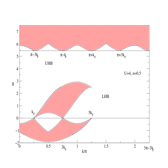
Figure 1: Regions of the ($k,\,\omega$)-plane where accordingly to the restrictions associated with the dominant holon and spinon microscopic processes studied in reference [16] there is a significant amount of one-electron spectral weight for on-site repulsion $U=4t$, electronic density $n=1/2$, and spin density $m=0$. Note that an extended momentum scheme is used. The one-electron addition upper and lower Hubbard band spectral functions correspond to values of excitation energy such that $\omega>E_{u}$ and $0<\omega<E_{u}$, respectively.

¿From analysis of the energy spectrum of the excited states generated by dominant processes, one finds that the $M^{th}$ Hubbard band finite-spectral-weight region of the $(k,\,\omega)$-plane whose lower limit is located at the line $\omega=M\,E_{u}$ is for all values of $k$ separated from the next lower-limit line $\omega=[M+1]\,E_{u}$ of the $[M+1]^{th}$ Hubbard band by a region with nearly no spectral weight. The latter region of the $(k,\,\omega)$-plane is out of the range of the excitations generated by dominant processes. This holds for all few-electron spectral functions and is illustrated in Fig. 1 for the specific case of the one-electron spectral function. For on-site repulsion $U=4t$, electronic density $n=1/2$, and spin density $m=0$ the regions of the ($k,\,\omega$)-plane whose spectral weight is generated by dominant processes are shown in the figure by shaded areas. The dominant processes also include pseudoparticle particle-hole processes which lead to spectral weight both inside and outside but in the close vicinity of the shaded domains of Fig. 1. In that figure an extended momentum scheme centered at momentum $k=0$ (and $k=\pi$) is used for electron removal and the $M=0$ lower Hubbard band (and $M=1$ first upper Hubbard band). The one-electron addition upper and lower Hubbard band spectral functions correspond to values of excitation energy such that $\omega>E_{u}$ and $\omega>0$, respectively. Note that for all values of $k$ there is indeed a region with nearly no spectral weight located between the finite-weight regions corresponding to the $M=0$ and $M=1$ Hubbard bands. In the figure the one-electron removal spectral function corresponds to $\omega<0$. The figure shows the locations ($k=\pi-l\,k_{F},\,\omega=E_{u}$) for the four $l=\pm 1,\pm 3$ upper Hubbard band lower-limit points whose weight distribution is studied below. There are also two upper Hubbard band lower-limit points for $l=\pm 5$ which are not shown in the figure.

As in the case of the one-electron spectral weight represented in the figure, it occurs for all few-electron spectral functions that in the straight and horizontal lower limit upper Hubbard band lines ($k,\,\omega=M\,E_{u}$) of the $(k,\,\omega$)-plane there is finite spectral weight for a set of discrete momentum values only, as mentioned above. These discrete momentum values coincide with the momenta $k_{M}^{l}$ given in Eq. (10). The four momenta $k=\pi-l\,k_{F}$ where $l=\pm 1,\,\pm 3$ that are shown in Fig. 1 are examples of such momentum values. Each of these momentum values correspond to a different reduced J-CPHS ensemble subspace of the CPHS ensemble space spanned by states of rotated electron double occupation $M$ and with an occupancy of $M=M_{c,\,-1/2}$ $-1/2$ holons. Our scheme provides the weight distribution for small energies $(\omega-M\,E_{u})$ corresponding to regions of the ($k,\,\omega$)-plane just above such straight and horizontal lower-limit upper Hubbard band lines. For the straight and horizontal lines parallel to the lower-limit lines and corresponding to values of $\omega$ such that $(\omega-M\,E_{u})$ is small, there is finite spectral weight for small momentum domains centered around the set of momentum values $k=k_{M}^{l}$.

The correlation-function expressions obtained from standard conformal-field theory [19, 20] correspond to a specific limit of our scheme such that $M=0$. The corresponding low-energy edges result from ground-state transitions to $M_{c,\,-1/2}=M=0$ excited states. In figure 1 this corresponds to the finite-weight regions in the vicinity of the three points ($k=k_{F},\,\omega=0$), ($k=3k_{F},\,\omega=0$), and ($k=5k_{F},\,\omega=0$). In the following applications of our finite-energy method we do not consider weight distributions resulting from such low-energy transitions, which can be evaluated by means of two-component conformal-field theory [20]. Our studies are restricted to the weight distribution of each of the above spectral functions in the vicinity of finite-energy points associated creation of $-1/2$ Yang holons and/or $c\nu$ pseudoparticles of bare momentum $q\approx\pm q^{0}_{c\nu}=\pm[\pi-2k_{F}]$. The weight distributions resulting from creation of $c\nu$ pseudoparticles at other bare-momentum values appear at finite energy $\omega$ such that $(\omega-\omega_{HS})$ is finite. These weight distributions cannot be evaluated by our method and are studied elsewhere [9, 10, 16]. Below we find that several critical exponents which control the weight distribution in the vicinity of the first and second upper Hubbard band lower-limit points equal corresponding exponents that control the low-energy weight distributions studied in Ref. [20]. However, we note that in the figures that reference these exponents were plotted for finite values of the magnetic field whereas our study refers to zero field and magnetization.

Transitions from the ground state to excited states belonging to the same J-CPHS ensemble subspace are of the same type, whereas transitions of different type refer to excited states belonging to different J-CPHS ensemble subspaces. In some cases we extend this concept to pairs of J-CPHS ensemble subspaces with the same absolute momentum value for $k^{l}_{M}$.

4.3 ONE-ELECTRON ADDITION UPPER-HUBBARD BAND WEIGHT DISTRIBUTION

We start by considering addition of a spin-up electron. According to Eq. (12) and Eqs. (51) and (52) of Ref. [7] with $\Delta L_{s,\,-1/2}=0$ and $\Delta N_{s\nu}=0$ for $\nu>1$, in the case of the $M_{c,\,-1/2}=M=1$ type of transitions one has that $\Delta N_{c}=\Delta N_{s}=-1$ and $\Delta J_{s}=\pm 1/2$. There are two one-$-1/2$ Yang holon types of transitions and six one-$q=\pm q^{0}_{c1}=\pm[\pi-2k_{F}]$ $c1$ pseudoparticle types of transitions. For $m\rightarrow 0$ the number of momentum values $k=k_{1}^{l}$ associated with dominant processes such that $\omega=E_{u}$ is in the present case six. These momentum values read $\pi-l\,k_{F}$ where $l=\pm 1,\,\pm 3,\,\pm 5$. Indeed, two one-$-1/2$ Yang holon type of transitions and two of the six one-$q=\pm q^{0}_{c1}=\pm[\pi-2k_{F}]$ $c1$ pseudoparticle type of transitions have the same momentum and energy spectrum. Thus, they contribute to the same upper Hubbard band lower-limit weight distribution located around the points $(k=\pi\mp k_{F},\,\omega=E_{u})$. These are the two one-$-1/2$ Yang holon types of transitions such that $L_{c,\,-1/2}=1$, $\Delta J_{c}=0$, and $\Delta J_{s}=\pm 1/2$ and the two one-$q=\pm q^{0}_{c\nu}=\pm[\pi-2k_{F}]$ $c1$ pseudoparticle types of transitions such that $N_{c1}=1$, $\Delta J_{c}=\pm 1/2$, $J_{c1}=\pm 1/2$, and $\Delta J_{s}=\pm 1/2$. Two other upper Hubbard band lower-limit points are ($k=\pi\mp 3k_{F}$, $\omega=E_{u}$). The corresponding spectral weight is generated by types of transitions such that $N_{c1}=1$, $\Delta J_{c}=\pm 1/2$, $J_{c1}=\mp 1/2$, and $\Delta J_{s}=\mp 1/2$. Below we also study the weight distribution in the vicinity of these points. In their vicinity there is a smaller amount of spectral weight than in the vicinity of the above two former points. Finally, the weight located in the vicinity of the remaining two points is even smaller. It is generated by transitions such that $N_{c1}=1$, $\Delta J_{c}=\pm 1/2$, $J_{c1}=\mp 1/2$, and $\Delta J_{s}=\pm 1/2$. These two points are located at ($k=\pi\mp 5k_{F}$, $\omega=E_{u}$). In the following we study the weight distribution around the above six upper Hubbard band lower-limit points located at ($k=\pi-l\,k_{F},\,\omega=E_{u}$) where $l=\pm 1,\,\pm 3,\,\pm 5$.

Let us consider the limit $m\rightarrow 0$ where the spin-up and spin-down one-electron spectral functions have the same form. Use of the general expression (17) leads for excitation energy $\omega$ just above $E_{u}$ and momentum values $k=\pi-l\,k_{F}$ where $l=\pm 1,\,\pm 3,\,\pm 5$ to,

$${\rm Im}\,\chi_{1p}(\pi-l\,k_{F},\,\omega)\propto(\omega-E_{u})^{\zeta_{1p}^{|l|}}\,;\hskip 14.22636ptl=\pm 1,\,\pm 3,\,\pm 5\,.$$ (24)

In this case the general exponent (19) is given by,

$$\zeta_{1p}^{|l|}=-{3\over 2}+{1\over 2}\,\Bigl{[}\,[1/\sqrt{2K_{\rho}}]^{2}+[l\,\sqrt{2K_{\rho}}/2]^{2}\Bigr{]}\,;\hskip 14.22636ptl=\pm 1,\,\pm 3,\,\pm 5\,.$$ (25)

To reach this result we first evaluated the expression for general values of $m$ in terms of the parameters (40) of Appendix A. Use of the limiting values for these parameters given in the same Appendix then leads to expression (25). The same procedure is followed in the calculation of the $m\rightarrow 0$ weight distribution of the dynamical structure factor and singlet Cooper pair spectral function given below. Note that in the present case all the transitions leading to the weight distributions (24) involve creation of both a $c$ pseudoparticle hole and a $s$ pseudoparticle hole. Note also that the dependence on $n$ and $U/t$ of the exponent (25) occurs through the parameter $K_{\rho}$ only, as mentioned in the previous section. For $m=0$ this is a general property of the critical exponents that control the weight distribution in the vicinity of the upper-Hubbard bands lower limit. In contrast, the expressions of the exponents that control the weight distribution in the vicinity of the branch lines studied in Ref. [10] involve the momentum-dependent phase shifts defined in Ref. [8].

The exponent (25) is a function of $U/t$ which for electronic densities $n$ such that $0<n<1$ changes from $\zeta_{1p}^{|l|}\rightarrow(l^{2}-5)/4=-1,\,1,\,5$ for $l=\pm 1,\,\pm 3,\,\pm 5$, respectively, as $U/t\rightarrow 0$ to $\zeta_{1p}^{|l|}\rightarrow(l^{2}-8)/8=-7/8,\,1/8,\,17/8$ for $l=\pm 1,\,\pm 3,\,\pm 5$, respectively, as $U/t\rightarrow\infty$. Note that as the critical exponent (25) approaches $-1$ for $l=\pm 1$ as $U/t\rightarrow 0$ the spectral function behaves as given in Eq. (20). The exponents (25) are plotted in Figs. 2 (a) and (b) for $k=\pi\mp k_{F}$ and $k=\pi\mp 3k_{F}$, respectively, as a function of the electronic density $n$ and for different values of $U/t$. The $l=\pm 5$ exponent is not plotted in the figure. This exponent is larger than two and corresponds to regions of very little spectral weight. The exponents plotted in Fig. 2 are monotonous functions of $n$. The exponent $\zeta_{1p}^{1}$ is always negative and such that $-1\leq\zeta_{1p}^{1}\leq-7/8$ and is associated with a weight-distribution singularity. It increases for increasing values of $U/t$. For finite values of $U/t$ it is a function of the electronic density $n$ with a minimum for an intermediate value of $n$. The exponent $\zeta_{1p}^{3}$ is always positive and such that $1/8\leq\zeta_{1p}^{3}\leq 1$ and is associated with a weight-distribution edge. The exponent $\zeta_{1p}^{3}$ decreases for increasing values of $U/t$. For finite values of $U/t$ it is a function of the electronic density $n$ with a maximum for an intermediate value of $n$.

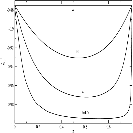
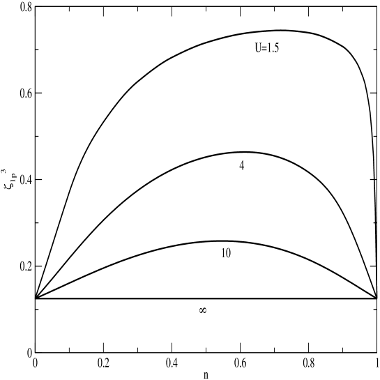
Figure 2: The upper Hubbard band one-electron exponents (a) $\zeta_{1p}^{1}$ and (b) $\zeta_{1p}^{3}$ given in Eq. (25) as a function of the electronic density $n$ for $U=1.5t$, $U=4t$, $U=10t$, and $U\rightarrow\infty$ (horizontal lines).

For all values of $U/t$ there is more spectral weight around the lower-limit upper Hubbard band points located at ($k=\pi\mp k_{F},\,\omega=E_{u}$) than around the points located at ($k=\pi\mp 3k_{F},\,\omega=E_{u}$). Moreover, the amount of weight in the vicinity of the points located at ($k=\pi\mp 3k_{F},\,\omega=E_{u}$) is larger than that of the weight located in the vicinity of the points ($k=\pi\mp 5k_{F},\,\omega=E_{u}$). For $U/t\rightarrow 0$ the spectral weight located in the vicinity of the points ($k=\pi\mp 3k_{F},\,\omega=E_{u}$) and ($k=\pi\mp 5k_{F},\,\omega=E_{u}$) disappears. As mentioned above, the value of the critical exponent plotted in Fig. 2 (a) is $-1$ for $U/t\rightarrow 0$. Thus, in this limit the spectral function behaves as given in expression Eq. (20). Importantly, in that limit the energy $E_{u}$ of the upper Hubbard band lower limit equals the non-interacting electronic spectrum at ($k=\pi\mp k_{F},\,\omega=E_{u}$). It follows that our general $U/t$ weight distribution leads to the correct non-interacting spectrum in the $U/t\rightarrow 0$ limit. In this paper we study the weight distribution in the vicinity of points located in the lower limit of the Hubbard bands. The branch-line studies of Ref. [10] reveal that the lower-Hubbard band and upper-Hubbard band spectral weights become connected at $k=\pi-k_{F}$ as $U/t\rightarrow 0$. For finite values of $U/t$, the finite-weight regions of these two bands are separated by a region out of the range of dominant processes. This is confirmed by analysis of Fig. 1.

Our above finite-energy expressions were derived for the metallic phase corresponding to electronic densities $0<n<1$. In the limit $n\rightarrow 1$ and finite values of $U/t$ expressions (25) lead to the correct $n=1$ results. In that limit and for $m\rightarrow 0$ the upper Hubbard band lower-limit points ($k=\pi\mp k_{F},\,\omega=E_{u}$) coincide with the lower-limit points ($k=\pi\mp 3k_{F},\,\omega=E_{u}$), and ($k_{=}\pi\mp 5k_{F},\,\omega=E_{u}$). Thus, in this case the smallest of the three exponents (25), such that $l=1$, controls the leading-order weight-distribution term (24).

In the limit $n\rightarrow 1$ the equality of the exponent that controls the electron removal lower-Hubbard band and the $l=\pm 1$ finite-energy electron addition exponent (25) is required by particle-hole symmetry. Our results reveal that in the metallic phase the $l=\pm 1$, $l=\pm 3$, and $l=\pm 5$ finite-energy exponents (25) also equal the exponents that control the weight distribution in the vicinity of the three zero-energy points located at ($k=\pm k_{F},\,\omega=0$), ($k=\pm 3k_{F},\,\omega=0$), and ($k=\pm 5k_{F},\,\omega=0$), respectively. (The points ($k=k_{F},\,\omega=0$), ($k=3k_{F},\,\omega=0$), and ($k=5k_{F},\,\omega=0$) are shown in Fig. 1.) For $l=\pm 1$ the exponent expression (25) was already found in Ref. [20]. It corresponds to the $H\rightarrow 0$ expressions of the one spin-up and spin-down electron exponents given in Table I of that reference, where $H$ is the magnetic field.

There are not many previous results about the excitation energy and momentum dependence of the weight distribution in the vicinity of the UHB lower-limit points considered above. Conformal-field theory does not apply to finite energy. The method used in Ref. [12] refers to $U/t\rightarrow\infty$ where the UHB lower limit corresponds to $\omega=E_{u}=\infty$. Thus, the UHB was not considered in the finite-energy studies of that reference. The point ($k=\pi-\,k_{F},\,\omega=E_{u}$) corresponds to ($k=\pi/2,\,(\omega-\mu)/t\approx 0.5$) and ($k=7\pi/12\approx 0.58\,\pi,\,(\omega-\mu)/t\approx 1$) in Figs. 3 and 4 of Ref. [13], respectively. The spectral weight of Fig. 3 is for half filling and $U/t=4$. (The figure zero-energy is the middle of the Mott-Hubbard gap.) The weight of Fig. 4 is for electronic density $n=5/6$ and $U/t=4$. These weight distributions were obtained by numerical calculations based on a combination of exact diagonalizations of finite clusters with strong-coupling perturbation theory and are consistent with our results. Unfortunately, a quantitative comparison is not possible because the method used in Ref. [13] does not provide accurate information about the weight-distribution dependence on the excitation energy and momentum.

4.4 THE DYNAMICAL STRUCTURE FACTOR UPPER-HUBBARD BAND WEIGHT DISTRIBUTION

According to Eq. (12) and Eqs. (51) and (52) of Ref. [7] with $\Delta L_{s,\,-1/2}=0$ and $\Delta N_{s\nu}=0$ for $\nu>1$, for $M_{c,\,-1/2}=M=1$ types of transitions one has in this case that $\Delta N_{c}=-2$, $\Delta N_{s}=-1$, and $\Delta J_{s}=0$. These transitions generate spectral weight in the vicinity of two upper Hubbard band lower-limit points. There are two one-$-1/2$ Yang holon types of transitions and two one-$q=\pm q^{0}_{c1}=\pm[\pi-2k_{F}]$ $c1$ pseudoparticle types of transitions which contribute to these weight distributions. The former two types of transitions correspond to $L_{c,\,-1/2}=1$ and $\Delta J_{c}=\pm 1/2$. The latter two types correspond to $N_{c1}=1$, $\Delta J_{c}=0$, and $J_{c1}=\mp 1/2$. The weight distribution in the vicinity of the two upper Hubbard band lower-limit points located at ($k=\pi\mp 2k_{F},\,\omega=E_{u}$) results from transitions belonging to these two types. Use of the general expression (17) leads in the limit $m\rightarrow 0$ to the following expression for the dynamical structure factor for excitation energy $\omega$ such that $(\omega-E_{u})$ is small and momentum values $k=\pi\mp 2k_{F}$,

$${\rm Im}\,\chi_{\rho}(\pi\mp 2k_{F},\,\omega)\propto(\omega-Eu)^{\zeta_{\rho}}\,.$$ (26)

¿From use of Eq. (19), we find the following expression for the critical exponent $\zeta_{\rho}$ in the limit $m\rightarrow 0$,

$$\zeta_{\rho}=-2\Bigl{[}1-[\sqrt{2K_{\rho}}/2]^{2}-[1/\sqrt{2K_{\rho}}]^{2}\Bigr{]}\,.$$ (27)

The exponent (27) is plotted in Fig. 3 as a function of the electronic density $n$ for different values of $U/t$. This exponent is a function of $U/t$ which for electronic densities densities $n$ such that $0<n<1$ and spin density $m=0$ changes from $\zeta_{\rho}\rightarrow 0$ as $U/t\rightarrow 0$ to $\zeta_{\rho}\rightarrow 1/2$ as $U/t\rightarrow\infty$. For the $n=1$ Mott-Hubbard insulator phase the exponent reads $1/2$ for all finite values of $U/t$. The exponent $\zeta_{\rho}$ is always positive and such that $0\leq\zeta_{\rho}\leq 1/2$ and is associated with a weight-distribution edge. It increases for increasing values of $U/t$. For finite values of $U/t$ it is a function of the electronic density $n$ with a minimum for an intermediate value of $n$.

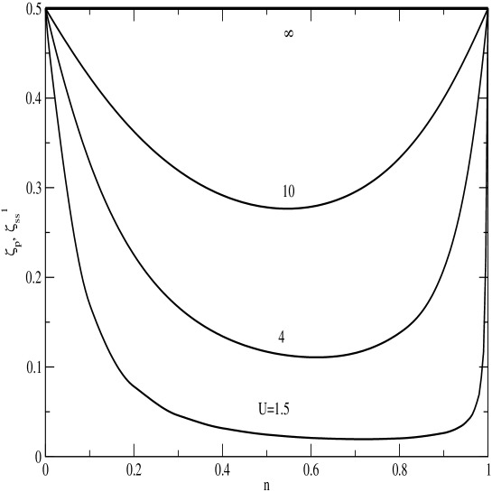
Figure 3: The exponents $\zeta_{\rho}=\zeta_{ss}^{1}$ (27) that control the weight distribution of the upper Hubbard band dynamical structure factor and second upper Hubbard band singlet Cooper pair spectral function, respectively, as a function of the electronic density $n$ for $U=1.5t$, $U=4t$, $U=10t$, and $U\rightarrow\infty$.

In contrast to the above one-electron problem, the spectral weight associated with the dynamical structure factor upper Hubbard band vanishes in the limit $U/t\rightarrow\infty$. For the $n=1$ Mott-Hubbard transition, the whole dynamical structure factor vanishes as $U/t\rightarrow\infty$. This behavior is related to the vanishing of the kinetic energy as $U/t\rightarrow\infty$ [21]. The dynamical structure factor upper Hubbard band exponent (27) had not been studied until now. It controls an onset of spectral weight whose $\omega$ derivative is infinite at the lower limit of the upper Hubbard band $\omega=E_{u}$ and raises upwards according to the power law (26).

In general the momentum values $k=\pi\mp 2k_{F}$ are finite and thus in the metallic phase the weight distribution (26) is not related to the zero-momentum frequency dependent optical conductivity. However, in the limit $n\rightarrow 1$ these momentum values vanish. Thus, for the particular case of the Mott-Hubbard insulator one can use the following relation between ${\rm Im}\,\chi_{\rho}(k,\,\omega)$ and the regular part of the frequency dependent optical conductivity $\sigma^{reg}(\omega)$,

$${\rm Re}\,\sigma^{reg}(\omega)\propto\lim_{k\rightarrow 0}{\omega\,{\rm Im}\,\chi_{\rho}(k,\,\omega)\over k^{2}}\,,$$ (28)

to find the ${\rm Re}\,\sigma^{reg}(\omega)$ weight distribution in the vicinity of the upper Hubbard band lower-limit point located at ($k=0,\,\omega=Eu=E_{MH}$). Use of this relation reveals that the exponent (27) controls the frequency dependence of that weight distribution. Combination of Eqs. (26) and (28) for $n\rightarrow 1$ and $E_{u}\rightarrow E_{MH}$ leads to,

$${\rm Re}\,\sigma^{reg}(\omega)\propto(\omega-E_{MH})^{1/2}\,.$$ (29)

This expression applies to all finite values of $U/t$.

In contrast to the upper Hubbard band dynamical structure factor expression (26) which refers to $k=\pi\mp 2k_{F}$ and values of $\omega$ such that $(\omega-E_{u})$ is small, the frequency dependence (29) of the $k=0$ optical conductivity in the vicinity of the upper Hubbard band lower-limit point was studied by other methods [14, 15]. In reference [14] that zero-momentum conductivity edge was studied for the metallic phase, whose critical exponent is different from the exponent (27). However, in the limit $n\rightarrow 1$ the zero-momentum density dependent exponent found in such a reference provides the correct half-filling exponent. In spite of the different method used in the evaluation of that exponent, the half-filling expression derived in Ref. [14] coincides with that of Eq. (29). Moreover, the same optical conductivity edge was studied in Ref. [15] for both small and large values of $U/t$. These investigations also lead to the same critical exponent $1/2$ for both these limits, in agreement with expression (29) which is valid for all finite values of $U/t$. As the conductivity exponent $-1/2$ is characteristic of a finite-energy semiconductor edge, also the conductivity exponent $1/2$ is now believed to be an universal signature of the Mott-Hubbard insulator [14, 15].

4.5 SPIN-SINGLET COOPER-PAIR FIRST AND SECOND UPPER-HUBBARD BAND WEIGHT DISTRIBUTIONS

The energy $E_{u}$ becomes small for low values of $U/t$ and electronic densities $n$ in the vicinity of one. Thus, it is interesting to clarify whether there are singular spectral features in the Cooper-pair spectral function at the upper-Hubbard bands lower limit. Indeed, for the above values of $U/t$ and electronic density such singular features could lead to a superconductivity instability for a system of weakly coupled Hubbard chains. Unfortunately, the only singular feature found below is a $\delta$ function peak located at the point $(k=\pi,\,\omega=E_{u})$. That isolated peak results from the $\eta$-pairing mechanism [17]. As the electronic density $n$ approaches one the weight of that peak vanishes as $(1-n)$. While this spectral structure cannot lead to a superconductivity instability for the coupled-chain system, other singular features for excitation energy above the first upper Hubbard band lower limit could exist, as further discussed in Sec. V.

According to Eqs. (12) and Eqs. (51) and (52) of Ref. [7] with $\Delta L_{s,\,-1/2}=0$ and $\Delta N_{s\nu}=0$ for $\nu>1$, in the case of the $M_{c,\,-1/2}=M=1$ type of transitions there is for the spin-singlet Cooper-pair spectral function a one-$-1/2$ Yang holon type of transition and three one-$q=\pm q^{0}_{c1}=\pm[\pi-2k_{F}]$ $c1$ pseudoparticle types of transitions. However, we find that the one-$q=\pm q^{0}_{c1}=\pm[\pi-2k_{F}]$ $c1$ pseudoparticle transition whose excitation momentum and energy is the same as the momentum and energy of the one-$-1/2$ Yang holon type of transition does not contribute to the singlet Cooper pair spectral function. Thus, only the one-$-1/2$ Yang holon type of transition and two of the three one-$q=\pm q^{0}_{c1}=\pm[\pi-2k_{F}]$ $c1$ pseudoparticle types of transitions contribute to weight-distribution features. We find that the weight-distribution feature generated by the one-$-1/2$ Yang holon transition is a single $\delta$ peak located in the first upper Hubbard band lower limit at $k=\pi$ and $\omega=E_{u}$. The matrix element between the corresponding $c1$ pseudoparticle excited state with the same momentum $k=\pi$ and excitation energy $\omega=E_{u}$ and the ground state vanishes in this case. Therefore, this singlet Cooper pair spectral function feature results from the one-$-1/2$ Yang holon excited state only. There are also two first upper Hubbard band lower-limit points located at ($k=\pi\mp 4k_{F},\,\omega=E_{u}$) which are generated by one-$q=\pm q^{0}_{c1}=\pm[\pi-2k_{F}]$ $c1$ pseudoparticle transitions. Below we also study the weight distribution in the vicinity of these first Hubbard band lower-limit points.

For the one-$-1/2$ Yang holon transition we find that $\Delta N_{c}=\Delta N_{s}=\Delta J_{c}=\Delta J_{s}=0$. Thus, this is an example of a transition where the quantity (19) reads $\zeta_{ss}=-2$ and is not a critical exponent. Instead, the correlation function at that point of the $(k,\,\omega)$-plane is of the form given in Eq. (20) for all values of $U/t$ and reads,

$$\chi_{ss}(\pi,\,\omega)={C_{\rho}\over\omega-E_{u}-i\beta}\,,$$ (30)

where $\beta\rightarrow 0$ and $C_{\rho}\geq 0$ is a constant. It follows that the associated singlet Cooper pair spectral-function weight distribution is indeed of the type given in Eq. (20) and reads,

$${\rm Im}\chi_{ss}(\pi,\omega)=\pi\,C_{\rho}\,\delta(\omega-E_{u})\,.$$ (31)

The weight feature (31) can be obtained by direct evaluation of the matrix elements on the right-hand side of expression (21) for $\vartheta=ss$. That procedure confirms in this particular case the validity of the results obtained by our method. Moreover, direct calculation of the matrix elements reveals that for $k=\pi$ the expressions (30) and (31) do not refer to values of $\omega$ such that $(\omega-E_{u})$ is small only, but to all values of excitation energy $\omega$. Direct evaluation of the matrix elements also reveals that the constant $C_{\rho}$ of Eqs. (30) and (31) reads $C_{\rho}=[N_{a}-N]$ and vanishes for the Mott-Hubbard insulator.

In order to evaluate the matrix elements of expression (21) for $\vartheta=ss$ and in the particular case of the momentum value $k=\pi$, we note that the off diagonal generator ${\hat{S}}^{c}_{+}$ of the $\eta$-spin $SU(2)$ algebra given in Eq. (9) of Ref. [6] can be rewritten as follows,

$${\hat{S}}^{c}_{+}=\sum_{k^{\prime}}c^{\dagger}_{k^{\prime},\,\downarrow}\,c^{\dagger}_{\pi-k^{\prime},\,\uparrow}\,.$$ (32)

Application of that generator onto a ground state produces an excited state with a $-1/2$ Yang holon. The generator of the above transition corresponds to creation of that $-1/2$ Yang holon and involves the initial ground state and this single final excited state only. After normalization this excited state can be written as follows,

$$|\,L_{c,\,-1/2}=1\rangle={\sum_{k^{\prime}}c^{\dagger}_{k^{\prime},\,\downarrow}\,c^{\dagger}_{\pi-k^{\prime},\,\uparrow}\over\sqrt{N_{a}-N}}\,|\,GS\rangle\,.$$ (33)

The main point is that at $k=\pi$ the singlet superconductivity operator given in Eq. (22) reads,

$${\hat{\cal{O}}}_{ss}(\pi)={\hat{S}}^{c}_{+}=\sum_{k^{\prime}}c^{\dagger}_{k^{\prime},\,\downarrow}\,c^{\dagger}_{\pi-k^{\prime},\,\uparrow}\,.$$ (34)

Use of Eq. (34) in Eq. (21) reveals that for $k=\pi$ the correlation function expression results from the overlap of the ground state with the excited state (33) only. Thus, for $k=\pi$ only one matrix element between the ground state and the available excited states of momentum $k=\pi$ is finite. That matrix element corresponds to the state (33). It follows that for $k=\pi$ the singlet superconductivity correlation function and corresponding spectral function are indeed given by expressions (30) and (31) with $C_{\rho}=[N_{a}-N]$ for all values of $\omega$.

The one-$-1/2$ Yang holon state (33) is associated with the $\eta$-pairing mechanism [17]. That mechanism leads in the metallic phase to the $\delta$-function peak (31) in the singlet Cooper pair spectral function. Such a state possesses off-diagonal long-range order [17]. The corresponding $\delta$ peak is located at finite excitation energy. The $\delta$ peak (31) is absent in the case of the Mott-Hubbard insulator where $C_{\rho}=[N_{a}-N]\rightarrow 0$. This vanishing is required by a half-filling selection rule, since the ground-state $\eta$ spin value of the Mott-Hubbard insulator reads $S_{c}=0$. Note that the present transition is a mere rotation in $\eta$-spin space which conserves $S_{c}$ and leads to $\Delta S_{c}=0$ and $\Delta S_{c}^{z}=+1$. Thus, only for initial ground states such that $S_{c}\geq 1$ can this transition occur. This excludes both the Mott-Hubbard insulator ground state such that $S_{c}=0$ and the one-hole doped Mott-Hubbard insulator ground state such that $S_{c}=1/2$.

Next, we consider the weight distribution in the vicinity of the first upper Hubbard band lower-limit points generated by other $M_{c,\,-1/2}=M=1$ types of transitions. These transitions correspond to a region of little spectral weight and are such that $N_{c1}=1$, $\Delta J_{c}=\pm 1/2$, $J_{c1}=\mp 1/2$, and $\Delta N_{c}=\Delta N_{s}=\Delta J_{s}=0$. Use of the general expression (17) leads in the limit $m\rightarrow 0$ to the following expression for the spin singlet Cooper pair spectral function for momentum values $k=\pi\mp 4k_{F}$ and excitation energy $\omega$ such that $(\omega-E_{u})$ is small,

$${\rm Im}\,\chi_{ss}(\pi\mp 4k_{F},\,\omega)\propto(\omega-E_{u})^{\zeta_{ss}}\,.$$ (35)

This weight-distribution edge does not occur for the Mott-Hubbard insulator. From use of Eq. (19) we find the following expression for the critical exponent $\zeta_{ss}$ in the limit $m\rightarrow 0$,

$$\zeta_{ss}=-2\Bigl{[}1-[\sqrt{2K_{\rho}}]^{2}\Bigr{]}\,.$$ (36)

This exponent is a function of $U/t$ which for all electronic densities changes from $\zeta_{ss}\rightarrow 2$ as $U/t\rightarrow 0$ to $\zeta_{ss}\rightarrow 0$ as $U/t\rightarrow\infty$. Such a dependence on $U/t$ is continuous. (Since there is not much spectral weight in the vicinity of this edge feature, we do not plot the positive exponent (36).)

We close our study by considering the weight distribution in the vicinity of the $M_{c,-1/2}=M=2$ second upper Hubbard band lower-limit points located at excitation energy $\omega=2E_{u}$. We note that for the Mott-Hubbard insulator there is no first upper Hubbard band. In this case there is an energy gap which equals twice the Mott-Hubbard gap and separates the singlet Cooper pair removal and addition spectral functions. The latter function corresponds to the present second upper Hubbard band in the limit $n\rightarrow 1$.

The $M_{c,\,-1/2}=M=2$ types of transitions are such that $\Delta N_{c}=-2$, $\Delta N_{s}=-1$, and $\Delta J_{s}=0$. Interestingly, there are five different types of transitions which contribute to the same weight distribution in the vicinity of two points and lead to the same critical exponent. These five types of transitions are such that (a) $L_{c,\,-1/2}=2$ and $\Delta J_{c}=\pm 1/2$, (b) $L_{c,\,-1/2}=1$, $N_{c1}=1$, $\Delta J_{c}=0$, $J_{c1}=\pm 1/2$, (c) $N_{c1}=2$, $\Delta J_{c}=\pm 1/2$, $J_{c1}=0$, (d) $N_{c1}=2$, $\Delta J_{c}=\pm 1/2$, $J_{c1}=\pm 1$, and (e) $N_{c,\,2}=1$, $\Delta J_{c}=0$, $J_{c1}=\pm 1/2$. All transitions of these types contribute to the weight distribution around the two second upper Hubbard band lower-limit points located at ($k=\pm 2k_{F},\,\omega=2E_{u}$). In addition, there is a sixth type of transition which leads to two second upper Hubbard band lower-limit points located at ($k=\pm 6k_{F},\,\omega=2E_{u}$). This type of transition is such that $N_{c1}=2$, $\Delta J_{c}=\pm 1/2$, and $J_{c1}=\mp 1/2$. There is nearly no spectral weight in the vicinity of these two latter points.

Use of the general expression (17) leads in the limit $m\rightarrow 0$ to the following expression for the spin singlet Cooper pair spectral function for excitation energy $\omega$ such that $(\omega-2E_{u})$ is small and momentum values $k=k_{2}^{l}=l\,2k_{F}$ where $l=\pm 1,\,\pm 3$,

$${\rm Im}\,\chi_{ss}(l\,2k_{F},\,\omega)\propto(\omega-2E_{u})^{\zeta_{ss}^{|l|}}\,;\hskip 14.22636ptl=\pm 1,\,\pm 3\,.$$ (37)

¿From use of Eq. (19), we find the following expression for the critical exponent $\zeta_{ss}^{|l|}$ in the limit $m\rightarrow 0$,

$$\zeta_{ss}^{|l|}=-2\Bigl{[}1-[l\,\sqrt{2K_{\rho}}/2]^{2}-[1/\sqrt{2K_{\rho}}]^{2}\Bigr{]}\,;\hskip 14.22636ptl=\pm 1,\,\pm 3\,.$$ (38)

Note that for $l=\pm 1$ this exponent equals the dynamical structure factor exponent $\zeta_{\rho}$ given in Eq. (27). Thus, it changes from $\zeta_{ss}^{1}\rightarrow 0$ as $U/t\rightarrow 0$ to $\zeta_{ss}^{1}\rightarrow 1/2$ as $U/t\rightarrow\infty$. It is plotted in Fig. 3 as a function of the electronic density $n$ for different values of $U/t$. On the other hand, the exponent $\zeta_{ss}^{3}$ is much larger and changes from $\zeta_{ss}^{3}\rightarrow 8$ as $U/t\rightarrow 0$ to $\zeta_{ss}^{1}\rightarrow 9/2$ as $U/t\rightarrow\infty$. This exponent corresponds to a region of very little spectral weight. In the limit $n\rightarrow 1$ the four second upper Hubbard lower-limit points located at ($k=\pm 2k_{F},\,\omega=2E_{u}$) and ($k=\pm 6k_{F},\,\omega=2E_{u}$) become the same single point. Thus, in this case the smaller exponent $\zeta_{ss}^{1}$ corresponds to the dominant contribution and controls the weight distribution in the vicinity of the lower-limit point located at ($k=\pi,\,\omega=2Eu=2E_{MH}$). For the $n=1$ Mott-Hubbard insulator phase the exponent $\zeta_{ss}^{1}$ reads $1/2$ for all finite values of $U/t$. It equals the exponent which controls the weight distribution around the zero-energy point located at ($k=\pi,\,\omega=0$). Interestingly, comparison with the results of Ref. [20] reveals that also in the metallic phase the exponents (38) for $l=\pm 1$ and $l=\pm 3$ equal the corresponding exponent that control the low-energy weight distribution of the singlet Cooper pair removal spectral function in the vicinity of the zero-energy points located at ($k=\pm 2k_{F},\,\omega=0$) and ($k=\pm 6k_{F},\,\omega=0$), respectively. However, in the metallic phase there is more spectral weight in the vicinity of the latter zero-energy points than in the vicinity of the corresponding second upper Hubbard band lower-limit points.

Finally, we note that if one extends the present study to finite-energy excited states with finite occupancies of $-1/2$ HL spinons and/or $s\nu$ pseudoparticles belonging to $\nu>1$ branches, similar features are obtained for gapped spin excitations. For instance, in the case of the spin-down triplet superconductivity spectral function a $\delta$-function peak similar to (31) is obtained at $k=\pi$ and $\omega=E_{u}+\mu_{0}\,H$. This peak is generated by a transition from the ground state to a single finite-energy excited state with one $-1/2$ Yang holon and one $-1/2$ HL spinon.

5 CONCLUDING REMARKS

In this paper we derived general few-electron spectral function expressions for the 1D Hubbard model in the vicinity of the lower limit of the upper Hubbard bands. For the one electron addition and dynamical structure factor we studied the weight distribution in the vicinity of the lower limit of the first upper Hubbard band. In the case of the singlet Cooper pair spectral function we considered the same problem in the vicinity of the lower limits of both the first and second upper bands. The weight of these Hubbard bands is generated by dominant holon and spinon processes which amount to more than 99% of the spectral weight [16]. Our general expressions were obtained by combination of symmetries of the 1D Hubbard model, such as the holon and spinon numbers conservation laws, with the finite-energy holon and spinon description of the quantum problem recently introduced in Refs. [6, 8].

The results obtained in this paper provide physically interesting and useful information about the finite-energy spectral properties of the present many-electron 1D quantum liquid and are complementary to the branch line studies of Refs. [9, 10, 16]. In the case of the one-electron problem the combination of our results with those of Ref. [10] provides all finite-energy spectral-weight singularities. Since the singular spectral features observed in quasi-1D metals agree quantitatively with the model singular branch lines, our results are of interest for the further understanding of the unusual spectral properties observed in low-dimensional materials [2, 4, 5, 9, 10]. Moreover, from the finite-energy weight-distribution found for the dynamical structure factor, we checked that in the limit of half filling our results lead for all finite values of $U/t$ to the expected Mott-Hubbard insulator exponent $1/2$ for the onset of the finite-frequency optical conductivity absorption. Unfortunately, we found no singular features at the the upper-Hubbard bands lower limit of the spin-singlet Copper-pair spectral function other than the expected $\eta$-pairing $\delta$-function peak. However, it could be that there are branch lines just above such a lower limit which show singular spectral features. Since the energy width of the first Hubbard band is small for low values of $U/t$ and electronic densities $n$ in the vicinity of one, such singular features could lead to an instability for a system of weakly coupled Hubbard chains. We thus suggest that this problem is further studied by the branch-line method used in Ref. [10] for the one-electron problem.

Appendix A THE FINITE-SIZE ENERGY SPECTRUM QUANTITIES

In this Appendix we show that the functional $2\,\Delta^{\iota}_{\alpha}$ has the form given in Eq. (15) and discuss issues related to the vanishing of the $c\nu$ finite-size energy spectrum for $q=\pm q^{0}_{c\nu}=\pm[\pi-2k_{F}]$.

By direct use of the results of Ref. [8], we find that for the excited states that span the reduced J-CPHS ensemble subspaces ${\cal H}_{red}$ the functional (14) can be written as,

$$2\,\Delta^{\iota}_{\alpha} = \Bigl{[}\iota\sum_{\alpha^{\prime}=c,s}\,\xi^{0}_{\alpha,\,\alpha^{\prime}}\,{\Delta N_{\alpha^{\prime}}\over 2}+\iota\sum_{\nu=1}^{\infty}\,\xi^{0}_{\alpha,\,c\nu}\,{N_{c\nu}\over 2}$$ (39)

$$+ \,\sum_{\alpha^{\prime}=c,s}\,\xi^{1}_{\alpha,\,\alpha^{\prime}}\,\Delta J_{\alpha^{\prime}}-\sum_{\nu=1}^{\infty}\,\xi^{1}_{\alpha,\,c\nu}\,J_{c\nu}\Bigr{]}^{2}\,.$$

Here the parameters $\xi^{j}_{\alpha,\,\alpha^{\prime}}$ and $\xi^{j}_{\alpha,\,c\nu}$ can expressed in terms of the two-pseudofermion phase shifts defined in Ref. [8] as follows,

$$\xi^{j}_{\alpha,\,\alpha^{\prime}} = \delta_{\alpha,\,\alpha^{\prime}}+\sum_{l=\pm 1}(l^{j})\,\Phi_{\alpha,\,\alpha^{\prime}}(q^{0}_{F\alpha},\,l\,q^{0}_{F\alpha^{\prime}})\,$$

$$\xi^{j}_{\alpha,\,c\nu} = \sum_{l=\pm 1}(l^{j})\,\Phi_{\alpha,\,c\nu}(q^{0}_{F\alpha},\,l\,[\pi-2k_{F}])\,.$$ (40)

In the limit $m\rightarrow 0$ these parameters read $\xi^{0}_{c,\,c}=1/\sqrt{2K_{\rho}}$, $\xi^{0}_{c,\,s}=0$, $\xi^{0}_{s,\,c}=-1/\sqrt{2}$, $\xi^{0}_{s,\,s}=\sqrt{2}$, $\xi^{0}_{c,\,c\nu}=0$, $\xi^{0}_{s,\,c\nu}=0$, $\xi^{1}_{c,\,c}=\sqrt{2K_{\rho}}$, $\xi^{1}_{c,\,s}=\sqrt{K_{\rho}/2}$, $\xi^{1}_{s,\,c}=0$, $\xi^{1}_{s,\,s}=1/\sqrt{2}$, $\xi^{1}_{c,\,c\nu}=\sqrt{2K_{\rho}}$, and $\xi^{1}_{s,\,c\nu}=0$. Here $K_{\rho}$ is the parameter defined in Ref. [22] which is such that $K_{\rho}\rightarrow 1$ as $U/t\rightarrow 0$ and $K_{\rho}\rightarrow 1/2$ as $U/t\rightarrow\infty$.

The creation of $-1/2$ Yang holons does not lead to any contribution to the value of the functional (39). However, the creation of $c\nu$ pseudoparticles leads to contributions through the terms $\iota\sum_{\nu=1}^{\infty}\,\xi^{0}_{\alpha,\,c\nu}\,N_{c\nu}/2$ and $-\sum_{\nu=1}^{\infty}\,\xi^{1}_{\alpha,\,c\nu}\,J_{c\nu}$ of that functional. On the other hand, the symmetry discussed in the text below Eq. (15) requires that the values of the phase-shift parameters $\xi^{j}_{\alpha,\,c\nu}$ of Eq. (40) are such that the functional (39) simplifies to (15). Indeed, by manipulation of the integral equations of Ref. [8] that define the two-pseudofermion phase shifts, we find the following relation between the parameters $\xi^{j}_{\alpha,\,c\nu}$ and $\xi^{1}_{\alpha,\,c}$ defined in Eq. (40),

$$\xi^{j}_{\alpha,\,c\nu}=j\,\xi^{1}_{\alpha,\,c}\,;\hskip 14.22636pt\alpha=c,\,s\,;\hskip 8.5359pt\nu=1,\,2,\,3,...\,;\hskip 8.5359ptj=0,\,1\,.$$ (41)

Use of this relation in Eq. (39) leads to (15).

Moreover, the same symmetry is behind the vanishing of the finite-size energy contributions of the $\pm q^{0}_{c\nu}=\pm[\pi-2k_{F}]$ $c\nu$ pseudoparticles. Indeed, by careful analysis of the general energy spectrum $\Delta E_{GL}$ we find that these contributions vanish provided that the quantity,

$$2\,\Delta^{\iota}_{c\nu}=\Bigl{[}{N_{a}\over 2\pi}\,\Bigl{(}\iota\,\Delta q^{0}_{c\nu}+{Q_{c\nu}(\iota\,q^{0}_{c\nu})\over N_{a}}\Bigr{)}\Bigr{]}^{2}\,;\hskip 14.22636pt\nu=1,2,...\,;\hskip 8.5359pt\iota=\pm 1\,,$$ (42)

also vanishes. Here $Q_{c\nu}(q)$ is the functional defined by Eq. (73) of Ref. [8]. Use of the equality $Q_{c\nu}(\iota\,q^{0}_{c\nu})/N_{a}=-\iota\,\Delta q^{0}_{c\nu}$ given in Eq. (126) of the same reference in expression (42) confirms that $2\,\Delta^{\iota}_{c\nu}$ vanishes for the excited states that span the reduced subspace.

These properties apply only to $c\nu$ pseudoparticles such that $q\rightarrow\pm[\pi-2k_{F}]$. Indeed, these quantum objects become non-interacting and localized in that limit. This behavior is related to the fact the $-1/2$ Yang holon is also non-interacting and invariant under the electron - rotated-electron unitary transformation [7]. However, in general a $c\nu$ pseudoparticle is different from the rotated $c\nu$ pseudoparticle. The only exception is precisely for bare momentum values $q$ such that $q\rightarrow\pm q^{0}_{c\nu}=\pm[\pi-2k_{F}]$. The $c\nu$ pseudoparticles become non-interacting in that limit only. Indeed, the energy associated with creation of a $-1/2$ Yang holon is given by $E_{u}$. A $c\nu$ pseudoparticle is a composite quantum object of $\nu$ $-1/2$ holons and $\nu$ $+1/2$ holons. Creation of a $+1/2$ holon is a process which requires no energy. The amount of energy required for creation of a $c\nu$ pseudoparticle is $\nu\,E_{u}+\epsilon^{0}_{c\nu}(q)$. Thus, the energy per $-1/2$ holon is $E_{u}+\epsilon^{0}_{c\nu}(q)/\nu\neq E_{u}$. However, one has that $\epsilon^{0}_{c\nu}(q)\rightarrow 0$ as $q\rightarrow\pm q^{0}_{c\nu}=\pm[\pi-2k_{F}]$ and thus in this limit the energy per $-1/2$ holon becomes $E_{u}$ and equals that of a non-interacting $-1/2$ Yang holon.

Appendix B THE FINITE-ENERGY CORRELATION FUNCTION

Here we show that the asymptotic expansion of the correlation function $\langle GS|\,{\hat{\phi}}_{\vartheta}(x,\,t)\,{\hat{\phi}}_{\vartheta}(0,0)\,|\,GS\rangle$ is of the form given in Eq. (16). The operator ${\hat{\phi}}^{GL}_{\vartheta}(x,\,t)$ acts and is defined in a reduced J-CPHS ensemble subspace associated with small values of the excitation energy $\Delta E_{GL}=(\omega-\omega_{HS})$ and excitation momentum $\Delta P_{GL}=(k-k_{M}^{l})$. In the Heisenberg description and in that reduced Hilbert subspace the space coordinate $x$ and time $t$ dependent physical field ${\hat{\phi}}^{GL}_{\vartheta}(x,\,t)$ can be expressed relative to its $x=0$ and $t=0$ expression ${\hat{\phi}}_{\vartheta}(0,\,0)$ as,

$${\hat{\phi}}^{GL}_{\vartheta}(x,\,t)=e^{-i[:\hat{H}_{GL}:\,t-:\hat{P}_{GL}:\,x]}\,{\hat{\phi}}_{\vartheta}(0,\,0)\,e^{i[:\hat{H}_{GL}:\,t-:\hat{P}_{GL}:\,x]}\,.$$ (43)

For the Hamiltonian $:{\hat{H}}_{GL}:$ of Eq. (6) the low-energy energy spectrum (13) and momentum spectrum $\Delta P_{GL}={2\pi\over N_{a}}\,\sum_{\alpha=c,s}\,\sum_{\iota=\pm 1}\,\iota\,[\,\Delta^{\iota}_{\alpha}+N^{ph}_{\alpha,\,\iota}]$ are conformal invariant and correspond to a two-component conformal-field theory associated with the $c$ and $s$ pseudoparticle excitation branches [19, 20]. The effect of the $c\nu$ pseudoparticles is merely to shift the $c$ pseudoparticle current number deviations $\Delta J_{c}$ by $-\sum_{\nu=1}^{\infty}J_{c\nu}$. Fortunately, such an effect does not affect the conformal invariance of the low-energy energy spectrum and momentum spectrum. Thus, the asymptotic expression for the low-energy correlation function of the physical field ${\hat{\phi}}^{GL}_{\vartheta}(x,\,t)$ is for electronic and spin densities such that $0<n<1$ and $0<m<n$, respectively, of the following general form [19, 20],

$$\langle GS|{\hat{\phi}}_{\vartheta}^{GL}(x,\,t)\,{\hat{\phi}}_{\vartheta}^{GL}(0,\,0)|GS\rangle\propto\prod_{\alpha=c,\,s}\,\prod_{\iota=\pm 1}{1\over(x-\iota v_{\alpha}\,t)^{2\Delta^{\iota}_{\alpha}}}\,.$$ (44)

We recall that the 1D Hubbard model $:\hat{H}:$ and Hamiltonian $:{\hat{H}}_{GL}:$ of Eq. (6) refer to the same ground state. Thus, the field ${\hat{\phi}}_{\vartheta}(x,\,t)$ is such that,

$${\hat{\phi}}_{\vartheta}(x,\,t)=e^{-i[:\hat{H}:\,t-:\hat{P}:\,x]}\,{\hat{\phi}}_{\vartheta}(0,\,0)\,e^{i[:\hat{H}:\,t-:\hat{P}:\,x]}\,,$$ (45)

where $:\hat{P}:$ is the momentum operator of Eq. (8). Since the Hamiltonians $:\hat{H}:$ and $:{\hat{H}}_{GL}:$ of Eq. (6) have the same energy eigenstates, there is a one-to-one correspondence between the correlation function terms (44) of the Hamiltonian $:{\hat{H}}_{GL}:$ and those of the 1D Hubbard model $:\hat{H}:$. Transitions to different reduced subspaces ${\cal{H}}_{red}$ lead to different correlation-function terms. Moreover, transitions to reduced subspaces with different values for $M\,E_{u}$ and $k_{M}^{l}$ lead for the 1D Hubbard model to correlation-function contributions with different values of the excitation energy $\omega\approx M\,E_{u}$ and momentum $k\approx k_{M}^{l}$. Thus, our first choice is the energy value $M\,E_{u}$ and momentum value $k_{M}^{l}$ which our correlation-function asymptotic term refers to. If for the same values of $M\,E_{u}$ and $k_{M}^{l}$ there are several reduced subspaces, we choose that associated with the leading-order asymptotic correlation-function term for the Hamiltonian $:{\hat{H}}_{GL}:$ of Eq. (6). That leading-order term is of the form (44). Let $|\,\psi(j)\rangle$ with $j=1,2,...$ denote the excited states that span the chosen reduced Hilbert subspace ${\cal{H}}_{red}$. Based on the commutation relations of the three normal-ordered Hamiltonians related by Eq. (6) and three normal-ordered momentum operators involved in Eq. (8) we find that,

$${\hat{\phi}}_{\vartheta}(x,\,t) = e^{-i[({\hat{H}}_{HS}+:{\hat{H}}_{GL}:)\,t-({\hat{P}}_{0}+:{\hat{P}}_{GL}:)\,x]}\,{\hat{\phi}}_{\vartheta}(0,\,0)\,e^{i[({\hat{H}}_{HS}+:{\hat{H}}_{GL}:)\,t-({\hat{P}}_{0}+:{\hat{P}}_{GL}:)\,x]}$$ (46)

$$= e^{-i[{\hat{H}}_{HS}\,t-{\hat{P}}_{0}\,x]}\,e^{-i[{:\hat{H}}_{GL}:\,t-:{\hat{P}}_{GL}:\,x]}{\hat{\phi}}_{\vartheta}(0,0)e^{i[{\hat{H}}_{GL}\,t-{\hat{P}}_{GL}\,x]}\,e^{i[{\hat{H}}_{HS}\,t-{\hat{P}}_{0}\,x]}$$

$$= e^{-i[{\hat{H}}_{HS}\,t-{\hat{P}}_{0}\,x]}\,{\hat{\phi}}_{\vartheta}^{GL}(x,\,t)e^{i[{\hat{H}}_{HS}\,t-{\hat{P}}_{0}\,x]}\,,$$

where we have used Eqs. (43) and (45). Equation (46) confirms that ${\hat{\phi}}_{\vartheta}(0,\,0)={\hat{\phi}}_{\vartheta}^{GL}(0,\,0)$.

Once the ground state has eigenvalue zero both for ${\hat{H}}_{HS}$ and ${\hat{P}}_{0}$ and all excited states that span the subspace ${\cal{H}}_{red}$ have for these operators the same eigenvalues $M\,E_{u}$ and $k_{M}^{l}$, respectively, we find that,

$$\langle GS|{\hat{\phi}}_{\vartheta}(x,\,t)\,{\hat{\phi}}_{\vartheta}(0,\,0)|GS\rangle$$ (47)

$$= \langle GS|\,e^{-i[{\hat{H}}_{HS}\,t-{\hat{P}}_{0}\,x]}\,{\hat{\phi}}_{\vartheta}^{GL}(x,t)\,e^{i[{\hat{H}}_{HS}\,t-{\hat{P}}_{0}\,x]}{\hat{\phi}}_{\vartheta}^{GL}(0,\,0)|GS\rangle$$

$$= \sum_{j}\langle GS|{\hat{\phi}}_{\vartheta}^{GL}(x,\,t)\,e^{i[{\hat{H}}_{HS}\,t-{\hat{P}}_{0}\,x]}\,|\psi(j)\rangle\langle\psi(j)|{\hat{\phi}}_{\vartheta}^{GL}(0,\,0)|GS\rangle$$

$$= e^{i[M\,E_{u}\,t-k_{M}^{l}\,x]}\,\langle GS|{\hat{\phi}}_{\vartheta}^{GL}(x,\,t)\,{\hat{\phi}}_{\vartheta}^{GL}(0,\,0)|GS\rangle\,.$$

Here the $j$ summation refers to the above set of excited states $\{|\psi(j)\rangle\}$ which span the suitable reduced subspace ${\cal{H}}_{red}$. Finally, the combination of Eqs. (44) and (47) implies that the leading term in the asymptotic expansion of the correlation function of the 1D Hubbard model is of the form given in Eq. (16).

References

References

- [1] Hussey N E, McBrien M N, Balicas L, Brooks J S, Horii S and Ikuta H 2002 Phys. Rev. Lett. 89, 086601
- [2] Menzel A, Beer R and Bertel E 2002 Phys. Rev. Lett. 89, 076803
- [3] Shin-ichi Fujimori, Akihiro Ino, Testuo Okane, Atsushi Fujimori, Kozo Okada, Toshio Manabe, Masahiro Yamashita, Hideo Kishida, and Hiroshi Okamoto 2002 Phys. Rev. Lett. 88, 247601
- [4] Hasan M Z, Montano P A, Isaacs E D, Shen Z-X, Eisaki H, Sinha S K, Islam Z, Motoyama N and Uchida S 2002 Phys. Rev. Lett. 88, 177403
- [5] Claessen R, Sing M, Schwingenschlögl U, Blaha P, Dressel M and Jacobsen C S 2002 Phys. Rev. Lett. 88, 096402.
- [6] Carmelo J M P, Román J M and Penc K 2004 Nucl. Phys. B at press (Preprint cond-mat/0302044)
- [7] Carmelo J M P and Sacramento P D 2003 Phys. Rev. B 68, 085104
- [8] Carmelo J M P 2003 Preprint cond-mat/0305568
- [9] Sing M, Schwingenschlögl U, Claessen R, Blaha P, Carmelo J M P, Martelo L M, Sacramento P D, Dressel M and Jacobsen C S 2003 Phys. Rev. B 68, 125111
- [10] Carmelo J M P, Penc K, Martelo L M, Sacramento P D, Lopes dos Santos J M B, Claessen R, Sing M and Schwingenschlögl U 2003 Preprint cond-mat/0307602
- [11] Lieb E H and Wu F Y 1968 Phys. Rev. Lett. 20, 1445; Takahashi M 1972 Prog. Theor. Phys. 47, 69
- [12] Karlo Penc, Karen Hallberg, Frédéric Mila, and Hiroyuki Shiba 1996 Phys. Rev. Lett. 77, 1390; 1997 Phys. Rev. B 55, 15 475
- [13] Sénéchal D, Perez D and Pioro-Ladrière M 2000 Phys. Rev. Lett. 84, 522
- [14] Carmelo J M P, Peres N M R and Sacramento P D 2000 Phys. Rev. Lett. 84, 4673
- [15] Jeckelmann E, Gebhard F and Essler F H L 2001 Phys. Rev. Lett. 85, 3910; Controzzi D, Essler F H L and Tsvelik A M 2001 Phys. Rev. Lett. 86, 680
- [16] Carmelo J M P and Penc K 2003 Preprint cond-mat/0311075
- [17] Heilmann O J and Lieb E H 1971 Ann. N. Y. Acad. Sci. 172, 583; Lieb E H 1989 Phys. Rev. Lett. 62, 1201; Yang C N 1989 Phys. Rev. Lett. 63, 2144
- [18] Brooks Harris A and Lange R V 1967 Phys. Rev. 157, 295
- [19] Belavin A A, Polyakov A M and Zamolodchikov A B 1984 Nucl. Phys. B 241, 333; Frahm H and Korepin V E 1990 Phys. Rev. B 42, 10 553
- [20] For a conformal field theory study of the critical exponents which control the ()-plane weight distribution in the vicinity of () low-energy edges see, Carmelo J M P, Guinea F and Sacramento P D 1997 Phys. Rev. B 55, 7565
-
[21]
Baeriswyl D, Carmelo J and Luther A 1986
Phys. Rev. B 33, 7247
Baeriswyl D, Carmelo J and Luther A 1986 Phys. Rev. B34, 8976 (erratum) - [22] Schulz H J 1990 Phys. Rev. Lett. 64, 2831