Excitation Spectrum of Bilayer $\nu=2$ Quantum Hall Systems

Abstract

Excitation spectra in bilayer quantum Hall systems at total Landau-level filling $\nu=2$ are studied by the Hartree-Fock-Bogoliubov approximation. The systems have the spin degrees of freedom in addition to the layer degrees of freedom described in terms of pseudospin. On the excitation spectra from spin-unpolarized and pseudospin-polarized ground state, this approximation fully preserves the spin rotational symmetry and thus can give not only spin-triplet but also spin-singlet excitations systematically. It is also found that the ground-state properties are well described by this approximation.

, and

1 Introduction

Strong interactions often drive low-dimensional systems into exotic new phases. For a two-dimensional electron system (2DES) under high perpendicular magnetic fields, the interaction dominates the system properties because the kinetic energy is quenched by the Landau-level quantization. One of the most interesting phenomena in this strongly-correlated system is the quantum Hall effect, which has attracted a great deal of experiment and theoretical interest [1]. Recent advances in material growth techniques have made it possible to fabricate high-quality 2DESs confined to two parallel layers. By the introduction of such layer degrees of freedom a lot of new correlation effects can be realized because the strength of interlayer interactions and interlayer tunneling are controllable [2].

In a bilayer quantum Hall (QH) system at total Landau-level filling $\nu=2$, theoretical [3]–[6] and experimental studies [7]–[9] have confirmed the existence of a canted antiferromagnetic phase (CAF) between a fully spin-polarized ferromagnetic phase and a spin-singlet one. The properties of low-lying excitations in this system have been discussed by the Hartree-Fock approximation (HF) [3] and exact diagonalization (ED) calculations [6]. However, the HF calculation neither preserves the spin rotational symmetry nor can well describe pseudospin correlations, while the ED calculation is only applicable to small-size systems. Thus, in order to investigate the excitation spectra of large-size systems, we adopt a better approximate approach called the Hartree-Fock-Bogoliubov (HFB) approximation [10, 11, 12], and then write down the effective Hamiltonian of the systems. This approximation can take particle-hole correlations into consideration better than the Hartree-Fock (HF) approximation and further preserves the spin and pseudospin rotational symmetries in contrast to insufficient treatment by the HF approximation. We discuss not only excitation spectra but also ground-sate properties based on this approximation.

2 Hartree-Fock-Bogoliubov Approach to Bilayer $\nu=2$ QH Systems

In the presence of interlayer tunneling in double-quantum-well structures, the single-particle states are split into symmetric and antisymmetric combinations of one-layer states. These layer degrees of freedom can be described in terms of pseudospin as $\sigma_{x}=\uparrow,\ \downarrow$. In the case of large interlayer-tunneling energy $\Delta_{\rm SAS}$ and small layer separation $d$ (typically $\Delta_{\rm SAS}/E_{C}\geq 0.6$ and $d/l_{B}\leq 1.0$, where $E_{C}=e^{2}/\epsilon l_{B}$ and $l_{B}=\sqrt{c\hbar/eB}$) considered in this paper, the ground state of bilayer $\nu=2$ QH system is spin-singlet and fully pseudospin polarized because the Zeeman energy is much smaller than the tunneling energy and the interaction energy. For simplicity we consider only the lowest Landau levels. We can write down the Hartree-Fock-Bogoliubov Hamiltonian in such case. We consider $N$-electron systems on a sphere [13] whose surface is passed through by $2S$ flux quanta, where $2S=N/2-1$ for $\nu=2$. The effective Hamiltonian is given by

$${\mathcal{H}}_{\rm eff} = {\mathcal{H}}_{0}+{\mathcal{H}}_{\pm},$$ (1)

$${\mathcal{H}}_{0} = \sum_{K,N}\bigl{\{}\,(\Delta_{\rm SAS}+e_{K}+\lambda_{K})(C_{KN}^{\dagger}C_{KN}+H_{KN}^{\dagger}H_{KN})$$ (2)

$$+\frac{\lambda_{K}}{2}(-1)^{N}(C_{KN}^{{\dagger}}C_{K,-N}^{{\dagger}}+H_{KN}^{{\dagger}}H_{K,-N}^{{\dagger}}+{\rm h.c.})$$

$$+f_{K}[C_{KN}^{\dagger}H_{KN}+(-1)^{N}C_{KN}^{\dagger}H_{K,-N}^{\dagger}+{\rm h.c.}]\,\bigl{\}},$$

$${\mathcal{H}}_{\pm} = \sum_{K,N}\bigl{[}(\Delta_{\rm SAS}+\Delta_{\rm Z}+e_{K}+\lambda_{K}-g_{K})D_{KN}^{\dagger}D_{KN}$$ (3)

$$+(\Delta_{\rm SAS}-\Delta_{\rm Z}+e_{K}+\lambda_{K}-g_{K})F_{KN}^{\dagger}F_{KN}$$

$$-g_{K}(-1)^{N}(D_{KN}^{\dagger}F_{K,-N}^{\dagger}+{\rm h.c.})\bigl{]},$$

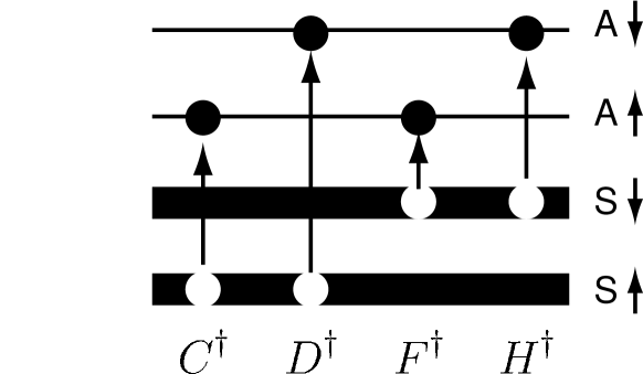
Figure 1: Excitons represented by operators $C^{{\dagger}}$, $D^{{\dagger}}$, $F^{{\dagger}}$, and $H^{{\dagger}}$. Energy levels occupied by electrons [ i.e., $S\uparrow$ (Symmetric and up-spin) and $S\downarrow$ (Symmetric and down-spin) levels ] are shown by thick lines, while solid and open circles indicate excited electrons into an unoccupied level [Antisymmetric and up-spin (or down-spin)] and holes in the $S\uparrow$ (or $S\downarrow$) levels, respectively. The changes in the $z$ component of total spin introduced by $C$, $D$, $F$ and $H$ excitons are $0$, $-1$, $+1$ and $0$, respectively.

$$e_{K}=\sum_{J=0}^{2S}(2J+1)V_{\rm intra}^{J}\left[\frac{(-1)^{2S-J}}{2S+1}-{SSJ\brace SSK}\right],$$

$$\lambda_{K}=\sum_{J=0}^{2S}(2J+1)\frac{V_{\rm intra}^{J}-V_{\rm inter}^{J}}{2}[(-1)^{2S-J}-1]{SSJ\brace SSK},$$

$$f_{K}=\sum_{J=0}^{2S}(2J+1)\frac{V_{\rm intra}^{J}-V_{\rm inter}^{J}}{2}(-1)^{2S-J}{SSJ\brace SSK},$$

$$g_{K}=f_{K}-\lambda_{K}.$$

Here ${\mathcal{H}}_{\rm eff}$ is composed of two parts, ${\mathcal{H}}_{0}$ and ${\mathcal{H}}_{\pm}$, described by such excitations that change the $z$ component of total spin by $0$ and $\pm 1$, respectively. $\Delta_{\rm SAS}$ is the energy gap between symmetric (S) and antisymmetric (A) single-particle states, and $\Delta_{\rm Z}$ is the Zeeman gap between spin up ($\uparrow$) and down ($\downarrow$) states. Because the system has the spatial rotational symmetry, the interaction matrix elements can be expressed in terms of Wigner’s $6j$ symbol ${SSJ\brace SSK}$ and intra/inter-layer pseudopotentials, $V^{J}_{\rm intra/inter}$ for relative angular momentum $2S-J$. $C^{{\dagger}}_{KN}$, $D^{{\dagger}}_{KN}$, $F^{{\dagger}}_{KN}$, and $H^{{\dagger}}_{KN}$ are exciton creation operators (see Fig.1). For example, $C^{{\dagger}}_{KN}=\sum_{l,m}\langle Sl;S,-m|KN\rangle a^{{\dagger}}_{l\uparrow}(-1)^{S-m}s_{m\uparrow}$ and this creates an exciton [a hole in the S $\uparrow$ level and a particle in the A $\uparrow$ level] with the total angular momentum $K$ and its $z$ component $N$, where $\langle Sl;S,-m|KN\rangle$ is the Clebsh-Gordan coefficient, and $a^{{\dagger}}_{l\sigma}$ ($s^{{\dagger}}_{m\sigma^{\prime}}$) creates an electron occupying the $l$ ($m$)-th antisymmetric (symmetric) combination of Landau orbits with spin-$\sigma$ ($\sigma^{\prime}$).

The diagonalization of ${\mathcal{H}}_{\pm}$ in Eqn.(3) can be performed by the following Bogoliubov transformation:

$${\mathcal{H}}_{\pm} = \sum_{K,N}\bigl{[}\,(\Delta_{\rm Z}+\omega_{K}^{T})R_{KN}^{{\dagger}}R_{KN}$$ (4)

$$\qquad+(-\Delta_{\rm Z}+\omega_{K}^{T})S_{KN}^{{\dagger}}S_{KN}\bigl{]},$$

$$\omega_{K}^{T} = \sqrt{(\Delta_{\rm SAS}+e_{\rm K})(\Delta_{\rm SAS}+e_{\rm K}-2g_{\rm K})}\,,$$

$$R_{KN} = D_{KN}\cosh{\frac{\phi_{K}}{2}}+(-1)^{N}F_{K,-N}^{{\dagger}}\sinh{\frac{\phi_{K}}{2}},$$

$$S_{K,-N} = (-1)^{N}D_{KN}^{{\dagger}}\sinh{\frac{\phi_{K}}{2}}+F_{K,-N}\cosh{\frac{\phi_{K}}{2}},$$

where $\tanh{\phi_{K}}=-g_{K}/(\Delta_{\rm SAS}+e_{K}-g_{K})$ and $\omega_{K}^{T}$ gives the energy of spin-triplet excitation.

The Hamiltonian ${\mathcal{H}}_{0}$ in Eqn.(2) can be decomposed into a spin-triplet part and a spin-singlet one. In fact, as linear combinations of operators $C_{KN}$ and $H_{KN}$, a new set of operators, $Q_{KN}$ and $P_{KN}$, can be introduced as $P_{KN}=(C_{KN}-H_{KN})/\sqrt{2}$, $Q_{KN}=(C_{KN}+H_{KN})/\sqrt{2}$, and then ${\mathcal{H}}_{0}$ can be written in terms of $Q_{KN}$ and $P_{KN}$ in the following form:

$${\mathcal{H}}_{0} = {\mathcal{H}}_{\rm triplet}^{0}+{\mathcal{H}}_{\rm singlet},$$ (5)

$${\mathcal{H}}_{\rm triplet}^{0} = \sum_{K,N}\bigl{[}\,(\Delta_{\rm SAS}+e_{K}-g_{K})P_{KN}^{{\dagger}}P_{KN}$$ (6)

$$-\frac{g_{K}}{2}(-1)^{N}(P_{KN}^{{\dagger}}P_{K,-N}^{{\dagger}}+{\rm h.c.})\bigl{]},$$

$${\mathcal{H}}_{\rm singlet} = \sum_{K,N}\bigl{[}(\Delta_{\rm SAS}+e_{K}+2\lambda_{K}+g_{K})Q_{KN}^{{\dagger}}Q_{KN}$$ (7)

$$+\frac{2\lambda_{K}+g_{K}}{2}(-1)^{N}(Q_{KN}^{{\dagger}}Q_{K,-N}^{{\dagger}}+{\rm h.c.})\bigl{]}.$$

Each part in Eqn.(5) can be diagonalized by the following Bogoliubov transformations, respectively, as

$${\mathcal{H}}_{\rm triplet}^{0} = \sum_{K,N}\omega_{K}^{T}\,T_{KN}^{{\dagger}}T_{KN},$$ (8)

$${\mathcal{H}}_{\rm singlet} = \sum_{K,N}\omega_{K}^{S}\,U_{KN}^{{\dagger}}U_{KN},$$ (9)

$$\omega_{K}^{S} = \sqrt{(\Delta_{\rm SAS}+e_{K})(\Delta_{\rm SAS}+e_{K}+4\lambda_{K}+2g_{K})}\,,$$

$$T_{KN} = P_{KN}\cosh{\frac{\phi_{K}}{2}}+(-1)^{N}P_{K,-N}^{{\dagger}}\sinh{\frac{\phi_{K}}{2}},$$

$$U_{KN} = Q_{KN}\cosh{\frac{\varphi_{K}}{2}}+(-1)^{N}Q_{K,-N}^{{\dagger}}\sinh{\frac{\varphi_{K}}{2}},$$

where $\tanh{\varphi_{K}}=(2\lambda_{K}+g_{K})/(\Delta_{\rm SAS}+e_{K}+2\lambda_{K}+g_{K})$, $\omega_{K}^{S}$ is the energy of spin-singlet excitation. The definitions of $\omega_{K}^{T}$ and $\phi_{K}$ have already been given on the diagonalization of ${\mathcal{H}}_{\pm}$ in Eqn.(4).

3 Results and Discussion

In Fig. 2 we show calculated results of excitation spectra in eight electron systems with $d/l_{B}=1.0$. Spin-triplet and spin-singlet excitation energies, $\omega_{K}^{T}$ and $\omega_{K}^{S}$, by HFB approximation are shown by open circles and squares, respectively. Calculated spectrum by the ED method is also shown by solid circles. Spin-triplet and spin-singlet excitations obtained by the ED method are linked by solid and dashed lines, respectively, as a guide to the eye. In the figure the contribution of the Zeeman energy to spin-triplet excitation energies is ignored, because it gives only constant shifts for excitation energies.

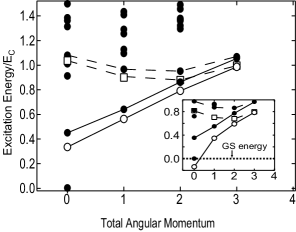
Figure 2: Low-lying excitation spectrum as a function of total angular momentum is shown for eight electrons, $d/l_{\rm B}=1$, and $\Delta_{\rm SAS}/E_{\rm C}=0.7$. Open circles (squares) linked by solid (dashed) line show the spin-triplet (-singlet) excitation spectrum by the HFB approximation. Excitation spectrum obtained by the ED method are shown by solid circles, and spin-triplet (-singlet) ones obtained by the ED method are linked by solid (dashed) lines as a guide to the eye. In the inset, the low-lying excitation spectrum for $\Delta_{\rm SAS}/E_{\rm C}=0.6$ is shown.

The HFB spectrum shows quantitative agreement with the ED results for large $\Delta_{\rm SAS}$ as $\Delta_{\rm SAS}/E_{C}=0.7$. On the other hand, for small $\Delta_{\rm SAS}$ the agreement between HFB and ED results becomes bad. For example, for $\Delta_{\rm SAS}/E_{C}=0.6$, the spin-triplet HFB spectrum shows a mode softening in the long wavelength limit overestimating the stability of the canted antiferromagnetic phase (shown in the inset of Fig. 2). We note that similar results are obtained for ten-electron systems.

In our HFB theory a spin-unpolarized (SU) and pseudospin-polarized (PP) state $|\Psi_{\rm SU-PP}\rangle=\prod_{m}s_{m\uparrow}^{{\dagger}}s_{m\downarrow}^{{\dagger}}|0\rangle$ is chosen as the reference state approximating the ground state. This state is the vacuum state of $C_{KN}$, $D_{KN}$, $F_{KN}$, $H_{KN}$, and in the HFB approximation these operators are treated as bosons. They are transformed by a series of Bogoliubov transformations and the ground state is obtained by applying these unitary transformations to $|\Psi_{\rm SU-PP}\rangle$. Then the ground state is characterized as the vacuum state of transformed bosons, $R_{KN}$, $S_{KN}$, $T_{KN}$ (three components of spin-triplet excitation), and $U_{KN}$ (spin-singlet one). Thus our HFB theory can systematically describe not only spin-triplet and spin-singlet excitations but also the ground state wavefunction. This is in striking contrast to the ambiguities in the HF theory.

In order to show clearly that the ground state properties are well described in our theory, the average number of electrons occupying antisymmetric single-particle states in ground state ($N_{A}$) is shown in Fig.3. In the HFB theory, this quantity is given by

$$N_{A}=\frac{1}{2}\sum_{K=0}^{2S}(2K+1)\left[3\sinh^{2}\biggl{(}\frac{\phi_{K}}{2}\biggl{)}+\sinh^{2}\biggl{(}\frac{\varphi_{K}}{2}\biggl{)}\right].$$

In the figure, calculated results by the ED, the effective spin theory, and the HF method are also shown in comparison with our result. It is found that for large tunneling energies the HFB approximation does reproduce the ED result better than the effective spin theory and the HF does.

On the other hand, for small tunneling energies as $\Delta_{\rm SAS}/E_{C}\leq 0.6$, the discrepancy between the ED and HFB theory becomes apparent and the effective spin theory shows a better agreement with the ED result than the HFB theory. This indicates that in small tunneling-energy region another reference state describing pseudospin correlations better is needed in our HFB theory.

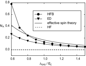
Figure 3: The average number of electrons occupying antisymmetric single-particle states in the ground state is shown as a function of $\Delta_{\rm SAS}/E_{\rm C}$ for eight electrons and $d/l_{\rm B}=1$.

4 Summary

Using the Hartree-Fock-Bogoliubov approximation, we have constructed an effective Hamiltonian for bilayer $\nu=2$ QH systems. This Hamiltonian preserves the spin rotational symmetry and gives both spin-singlet and spin-triplet excitations systematically in contrast to the Hartree-Fock method. In particular, in the large tunneling-energy region, our HFB theory describes the bilayer $\nu=2$ QH system better than other approximate theories. The ground-state properties are well described by our theory, too.

T.N. and A.S. acknowledge support by Grant-in-Aid for Scientific Research (Grant No.14740181 and No.14340088) by the Ministry of Education, Culture, Sports, Science and Technology of Japan, respectively.

References

[1]Quantum Hall Effect,
edited by R. E. Prange, S. M. Girvin
(Springer-Verlag, New York, 1987).
[2]Perspective in Quantum Hall Effects,
edited by S. Das Sarma, A. Pinczuk
(Wiley, New York, 1997).
[3] S. Das Sarma, S. Sachdev, L. Zheng,
Phys. Rev. Lett. 79, 917 (1997)
; Phys. Rev. B 58, 4672 (1998).
[4] A. H. MacDonald, R. Rajaraman,
T. Jungwirth, Phys. Rev. B 60, 8817 (1999).
[5] E. Demler, S. Das Sarma, Phys. Rev. Lett.
82, 3895 (1999).
[6] J. Schliemann, A. H. MacDonald,
Phys. Rev. Lett. 84, 4437 (2000).
[7] A. Sawada et al.,
Phys. Rev. Lett. 80, 4534 (1998).
[8] V. Pellegrini et al.,
Phys. Rev. Lett. 79, 310 (1997); Science 281, 799 (1998).
[9] V. S. Kharapai et al.,
Phys. Rev. Lett. 84, 725 (2000).
[10] On the Hartree-Fock-Bogoliubov theory,
see The Nuclear Many-body Problem,
by P. Ring, P. Schuck (Springer-Verlag, Berlin, 1980).
[11] N. N. Bogoliubov, Uspekhi fiz. Nauk.
67, 549 (1959)
[translation: Soviet Phys.-Uspekhi 67, 236 (1959)];
J. G. Valatin: Phys. Rev. 122, 1012 (1961).
[12] T. Nakajima, H. Aoki, Phys. Rev. B
56, R15549 (1997).
[13] Spherical systems are convenient to the theoretical
extension to the fractional filling
based on the composite-fermion picture:
X.G. Wu, J.K. Jain, Phys. Rev. B 49, 7515 (1994);
T. Nakajima, H. Aoki, Phys. Rev. B 52, 13780 (1995).