Random Walks on Complex Networks

Abstract

We investigate random walks on complex networks and derive an exact expression for the mean first passage time (MFPT) between two nodes. We introduce for each node the random walk centrality $C$, which is the ratio between its coordination number and a characteristic relaxation time, and show that it determines essentially the MFPT. The centrality of a node determines the relative speed by which a node can receive and spread information over the network in a random process. Numerical simulations of an ensemble of random walkers moving on paradigmatic network models confirm this analytical prediction.

From biology over computer science to sociology the world is abundant in networks. Watts and Strogatz Watts.Strogatz98 demonstrated that many of these real-world networks pose characteristic features like the small world and clustering property. Since classical network models do not display these features, new models have been developed to understand the structure underlying real-world networks  Albert.Barabasi02 ; Dorogovtsev.Mendes02 . The important finding is that there exists a scale-free (SF) network characterized by a power-law degree distribution Albert.Jeong.Barabasi99 , that is also a characteristic for the World-Wide-Web (WWW) Albert.Jeong.Barabasi99 , and for many other networks in various disciplines Albert.Barabasi02 .

The SF network has a heterogeneous structure. For instance, the WWW analyzed in Ref. Albert.Jeong.Barabasi99 includes nodes with degrees ranging from ${\cal O}(1)$ to ${\cal O}(10^{3})$. The heterogeneity leads to intriguing properties of SF networks. In the context of percolation, SF networks are stable against random removal of nodes while they are fragile under intentional attacks targeting on nodes with high degree Cohen.E.A.H00 ; Albert.Jeong.Barabasi00 . Statistical mechanical systems on SF networks also display interesting phase transitions Pastor-Satorras.Vespignani01 ; Dorogovtsev.Goltsev.Mendes02 ; Igloi.Turban02 . In a transport process, each node in SF networks does not contribute equally likely. The importance of each node in such a process is measured with the betweenness centrality Newman01 , which has a broad power-law distribution Goh01.02 .

In this paper, we study a random walk on general networks with a particular attention to SF networks. The random walk is a fundamental dynamic process Hughes95 . It is theoretically interesting to study how the structural heterogeneity affects the nature of the diffusive and relaxation dynamics of the random walk RWref . Those issues will be studied further elsewhere Noh.Rieger03 . The random walk is also interesting since it could be a mechanism of transport and search on networks Adamic.L.P.H01 ; Guimera.etal02 ; Holme03 . Those processes would be optimal if one follows the shortest path between two nodes under considerations. Among all paths connecting two nodes, the shortest path is given by the one with the smallest number of links comment1 . However the shortest path can be found only after global connectivity is known at each node, which is improbable in practice. The random walk becomes important in the extreme opposite case where only local connectivity is known at each node. We also suggest that the random walk is a useful tool in studying the structure of networks.

In the context of transport and search, the mean first passage time (MFPT) is an important characteristic of the random walk. We will derive an exact formula for the MFPT of a random walker from one node $i$ to another node $j$, which will be denoted by $\langle T_{ij}\rangle$, in arbitrary networks. In the optimal process it is just given by the number of links in the shortest path between two nodes, and both motions to one direction and to the other direction are symmetric. However, a random walk motion from $i$ to $j$ is not symmetric with the motion in the opposite direction. The asymmetry is characterized with the difference in the MFPT’s. It is revealed that the difference is determined by a potential-like quantity which will be called the random walk centrality (RWC). The RWC links the structural heterogeneity to the asymmetry in dynamics. It also describes centralization of information wandering over networks.

We consider an arbitrary finite network (or graph) which consists of nodes $i=1,\ldots,N$ and links connecting them. We assume that the network is connected (i.e. there is a path between each pair of nodes $(i,j)$), otherwise we simply consider each component separately. The connectivity is represented by the adjacency matrix ${\bf A}$ whose element $A_{ij}=1~{}(0)$ if there is a link from $i$ to $j$ (we set $A_{ii}=0$ conventionally). In the present work, we restrict ourselves to an undirected network, namely $A_{ij}=A_{ji}$. The degree, the number of connected neighbors, of a node $i$ is denoted by $K_{i}$ and given by $K_{i}=\sum_{j}A_{ij}$.

The stochastic process in discrete time that we study is a random walk on this network described by a master equation. The transition probabilities are defined by the following rule: A walker at node $i$ and time $t$ selects one of its $K_{i}$ neighbors with equal probability to which it hops at time $t+1$, thus the transition probability from node $i$ to node $j$ is $A_{ij}/K_{i}$ comment3 . Suppose the walker starts at node $i$ at time $t=0$, then the master equation for the probability $P_{ij}$ to find the walker at node $j$ at time $t$ is

$$P_{ij}(t+1)=\sum_{k}\frac{A_{kj}}{K_{k}}P_{ik}(t)\ .$$ (1)

The largest eigenvalue of the corresponding time evolution operator is $1$ corresponding to the stationary distribution $P_{j}^{\infty}=\lim_{t\to\infty}P_{ij}(t)$, i.e. the infinite time limit comment2 . An explicit expression for the transition probability $P_{ij}(t)$ to go from node $i$ to node $j$ in $t$ steps follows by iterating Eq. (1)

$$P_{ij}(t)=\sum_{j_{1},\ldots,j_{t-1}}\frac{A_{ij_{1}}}{K_{i}}\cdot\frac{A_{j_{1}j_{2}}}{K_{j_{1}}}\cdots\frac{A_{j_{t-1}j}}{K_{j_{t-1}}}\ .$$ (2)

Comparing the expressions for $P_{ij}$ and $P_{ji}$ one sees immediately that

$$K_{i}P_{ij}(t)=K_{j}P_{ji}(t)\ .$$ (3)

This is a direct consequence of the undirectedness of the network. For the stationary solution, Eq. (3) implies that $K_{i}P^{\infty}_{j}=K_{j}P_{i}^{\infty}$, and therefore one obtains

$$P_{i}^{\infty}=\frac{K_{i}}{{\cal N}}$$ (4)

with ${\cal N}=\sum_{i}K_{i}$. Note that the stationary distribution is, up to normalization, equal to the degree of the node $i$ — the more links a node has to other nodes in the network, the more often it will be visited by a random walker.

How fast is the random walk motion? To answer to this question, we study the MFPT. The first-passage probability $F_{ij}(t)$ from $i$ to $j$ after $t$ steps satisfies the relation

$$P_{ij}(t)=\delta_{t0}\delta_{ij}+\sum_{t^{\prime}=0}^{t}P_{jj}(t-t^{\prime})F_{ij}(t^{\prime})\ .$$ (5)

The Kronecker delta symbol insures the initial condition $P_{ij}(0)=\delta_{ij}$ ($F_{ij}(0)$ is set to zero). Introducing the Laplace transform $\tilde{f}(s)\equiv\sum_{t=0}^{\infty}e^{-st}f(t)$, Eq. (5) becomes $\widetilde{P}_{ij}(s)=\delta_{ij}+\widetilde{F}_{ij}(s)\widetilde{P}_{jj}(s)$, and one has

$$\widetilde{F}_{ij}(s)=(\widetilde{P}_{ij}(s)-\delta_{ij})/\widetilde{P}_{jj}(s)\ .$$ (6)

In finite networks the random walk is recurrent Hughes95 , so the MFPT is given by $\langle T_{ij}\rangle=\sum_{t=0}^{\infty}tF_{ij}(t)=-\widetilde{F}^{\prime}_{ij}(0)$.

Since all moments $R^{(n)}_{ij}\equiv\sum_{t=0}^{\infty}t^{n}~{}\{P_{ij}(t)-P_{j}^{\infty}\}$ of the exponentially decaying relaxation part of $P_{ij}(t)$ are finite, one can expand $\widetilde{P}_{ij}$ as a series in $s$ as

$$\widetilde{P}_{ij}(s)=\frac{K_{j}}{{\cal N}(1-e^{-s})}+\sum_{n=0}^{\infty}(-1)^{n}R^{(n)}_{ij}\frac{s^{n}}{n!}\ .$$ (7)

Inserting this series into Eq. (6) and expanding it as a power series in $s$, we obtain that

$$\langle T_{ij}\rangle=\left\{\begin{array}[]{cl}\frac{{\cal N}}{K_{j}},&\quad\mbox{ for }j=i\\[8.53581pt] \frac{{\cal N}}{K_{j}}\left[R^{(0)}_{jj}-R^{(0)}_{ij}\right],&\quad\mbox{ for }j\neq i\end{array}\right.\ .$$ (8)

A similar expression is derived in Ref. Hughes95 for the MFPT of the random walk in periodic lattices.

It is very interesting to note that the average return time $\langle T_{ii}\rangle$ does not depend on the details of the global structure of the network. It is determined only by the total number of links and the degree of the node. Since it is inversely proportional to the degree, the heterogeneity in connectivity is well reflected in this quantity. In a SF network with degree distribution $P(K)\sim K^{-\gamma}$, the MFPT to the origin $T_{o}$ also follows a power-law distribution $P(T_{o})\sim T_{o}^{-(2-\gamma)}$. The MFPT to the origin distributes uniformly in the special case with $\gamma=2$.

Random walk motions between two nodes are asymmetric. The difference between $\langle T_{ij}\rangle$ and $\langle T_{ji}\rangle$ for $i\neq j$ can be written as (using Eq. (8))

$$\langle T_{ij}\rangle-\langle T_{ji}\rangle={\cal N}\left(\frac{R^{(0)}_{jj}}{K_{j}}-\frac{R^{(0)}_{ii}}{K_{i}}\right)-{\cal N}\left(\frac{R_{ij}^{(0)}}{K_{j}}-\frac{R_{ji}^{(0)}}{K_{i}}\right),$$

where the last term vanishes due to Eq. (3). Therefore we obtain

$$\langle T_{ij}\rangle-\langle T_{ji}\rangle=C_{j}^{-1}-C_{i}^{-1},$$ (9)

where $C_{i}$ is defined as

$$C_{i}\equiv\frac{P_{i}^{\infty}}{\tau_{i}}\;,$$ (10)

where $P_{i}^{\infty}=K_{i}/{\cal N}$ and the characteristic relaxation time $\tau_{i}$ of the node $i$ is given by

$$\tau_{i}=R_{ii}^{(0)}=\sum_{t=0}^{\infty}\{P_{ii}(t)-P_{i}^{\infty}\}\ .$$ (11)

We call $C_{i}$ the random walk centrality since it quantifies how central a node $i$ is located regarding its potential to receive informations randomly diffusing over the network. To be more precise: Consider two nodes $i$ and $j$ with $C_{i}>C_{j}$. Assume that each of them launches a signal simultaneously, which is wandering over the network. Based on Eq. (9), one expects that the node with larger RWC will receive the signal emitted by its partner earlier. Hence, the RWC can be regarded as a measure for effectiveness in communication between nodes. In a homogeneous network with translational symmetry, all nodes have the same value of the RWC. On the other hand, in a heterogeneous network the RWC has a distribution, which leads to the asymmetry in the random dynamic process.

The RWC is determined by the degree $K$ and $\tau$. The order of magnitude of the characteristic relaxation time $\tau$ is related to the second largest eigenvalue (nota bene comment2 ) of the time evolution operator in (1): $P_{ii}(t)=P_{i}^{\infty}+\sum_{\lambda=2}^{N}a_{i}^{(\lambda)}b_{i}^{(\lambda)}\Lambda_{\lambda}^{t}$, where $a^{(\lambda)}$ and $b^{(\lambda)}$ are the left and right eigenvectors, respectively, of the time evolution operator belonging to the eigenvalue $\Lambda_{\lambda}$. If we order the eigenvalues according to the modulus ($|\Lambda_{2}|\geq|\Lambda_{3}|\geq\ldots\geq|\Lambda_{N}|$) the asymptotic behavior is $P_{ii}(t)-P_{i}^{\infty}\sim a_{i}^{(2)}b_{i}^{(2)}\Lambda_{2}^{t}$ and $\tau_{i}\approx a_{i}^{(2)}b_{i}^{(2)}/|\ln|\Lambda_{2}||$. Thus the relaxation time $\tau_{i}$ has a node dependence only through the weight factor, which is presumably weak. On the other hand, the degree dependence is explicit.

We examined the distribution of the RWC in the Barabási-Albert (BA) network Barabasi.Albert99 . This is a model for a growing SF network; at each time step, a new node is added creating $m$ links with other nodes which are selected with the probability proportional to their degree. We grew the network, solved the master equation numerically with the initial condition $P_{i}(t=0)=\delta_{ik}$, and calculated the relaxation time $\tau_{k}$ for each $k$. Figure 1 (a) shows the plot of $\tau$ vs. $K$ in the BA network of $N=10^{4}$ nodes grown with the parameter $m=2$. The degree is distributed broadly over the range $2\leq K\lesssim 400$. On the other hand, the relaxation time turns out to be distributed very narrowly within the range $1\lesssim\tau\lesssim 2$. We also studied BA networks of different sizes, but did not find any significant broadening of the distribution of $\tau$. So the RWC distribution is mainly determined by the degree distribution. In Fig. 1 (b) we show the plot of $C$ vs. $K$ in the same BA network. It shows that the RWC is roughly proportional to the degree. Note however that the RWC is not increasing monotonically with the degree due to the fluctuation of $\tau$ as seen in Fig. 1 (a).

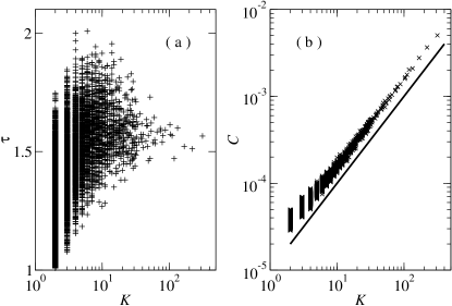
Figure 1: (a) $\tau$ vs. $K$ and (b) $C$ vs. $K$ calculated in the Barabási-Albert network with $N=10000$ and $m=2$. The straight line in (b) has the slope 1.

The RWC is useful when one compares the random walk motions between two nodes, e.g., $i$ and $j$ with $C_{i}>C_{j}$. On average a random walker starting at $j$ arrives at $i$ before another walker starting at $i$ arrives at $j$. Now consider an intermediate node $k$, which may be visited by both random walkers. Since $\langle T_{ij}\rangle>\langle T_{ji}\rangle$, it is likely that a random walker starting at node $k$ will arrive at node $i$ earlier than at node $j$. Although this argument is not exact since we neglected the time spent on the journey to the intermediate node, it indicates that nodes with larger RWC may be typically visited earlier than nodes with smaller RWC by the random walker. If we interpret the random walker as an information messenger, nodes with larger RWC are more efficient in receiving information than nodes with smaller RWC.

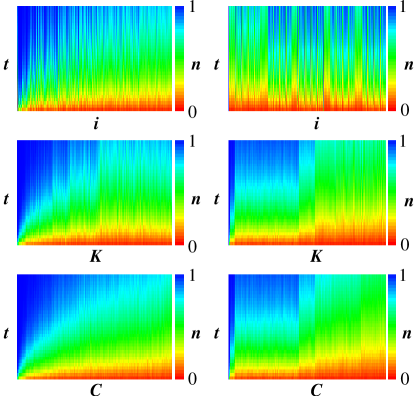
Figure 2: (Color online) Time evolution of the fraction of walkers $n$ that pass through a node as a function of (from top to bottom) the node index $i$, the node degree $K$ and the RWC $C$ of the BA network (left column) and the hierarchical network (right column). The value of $n$ at each time $t$ is represented in the gray scale/color code depicted at the right border of each plot.

We performed numerical simulations to study the relation between the RWC and this efficiency. To quantify it, we consider a situation where initially all nodes in a network are occupied by different random walkers. They start to move at time $t=0$, and we measure $n_{i}$, the fraction of walkers which have passed through the node $i$, as a function of time $t$. It is assumed that the walkers do not interact with each other. They may be regarded as a messenger delivering an information to each node it visits. Then, with the information distribution uniformly initially, $n_{i}$ is proportional to the amount of information acquired by each node. The argument in the previous paragraph suggests that typically nodes with larger values of RWC have larger value of $n_{i}$ at any given time.

The BA network Barabasi.Albert99 and the hierarchical network of Ravasz and Barabási cite:hnet were considered in the simulations. The hierarchical network is a deterministic network growing via iteration; at each iteration the network is multiplied by a factor $M$. The emergent network is scale-free when $M\geq 3$. Since it is a deterministic network, several structural properties are known exactly Noh03 . We measured $n_{i}$ in the BA network with $m=2$ and $N=512$ nodes and in the hierarchical network with $M=5$ and $N=5^{4}$ nodes for $0\leq t\leq 2048$, which are presented in the left and the right column of Fig. 2, respectively. The value of $n_{i}$ is color-coded according to the reference shown in Fig. 2.

The time evolution of $n_{i}$ is presented in three different ways. In the first row, the nodes are arranged in ascending order of the node index $i$. In the BA network, the node index corresponds to the time step at which the node is added to the network. The indexing scheme for the hierarchical network is explained in Ref. Noh03 . In the second row, the nodes are arranged in descending order of the degree $K$ and in the third row they are arranged in descending order of the RWC $C$. At a given time $t$, the plot in the first row shows that $n$ is non-monotonous and very irregular as a function of the node index. As a function of the degree it becomes smooth, but still non-monotonic tendencies remain. However, as a function of the RWC, it becomes much smoother and almost monotonous. We calculated for each node $i$ the time $\tau^{\prime}_{i}$ at which $n_{i}$ becomes greater than $1/2$. In the BA network, among all node pairs $(i,j)$ satisfying $\tau^{\prime}_{i}<\tau^{\prime}_{j}$, only $3\%$ violate the relation $C_{i}>C_{j}$, whereas the number of pairs that violate the relation $K_{i}>K_{j}$ is five times larger.

In summary, we studied the random walk processes in complex networks. We derive an exact expression for the mean first passage time (see Eq. (8)). The MFPT’s between two nodes differ for the two directions in general heterogeneous networks. We have shown that this difference is determined by the random walk centrality $C$ defined in Eq. (10). Among random walk motions between two nodes, the walk to the node with larger value of $C$ is faster than the other. Furthermore, it is argued that in a given time interval nodes with larger values of $C$ are visited by more random walkers which were distributed uniformly initially. We confirmed this by numerical simulations on the BA and the hierarchical network. One may regard the random walkers as informations diffusing through the network. Our results imply that information does not distribute uniformly in heterogeneous networks; the information is centralized to nodes with larger values of $C$. The nodes with high values of $C$ have the advantage of being aware of new information earlier than other nodes. On the other hand, it also implies that such nodes are heavily loaded within an information distribution or transport process. If the network has a finite capacity, the heavily loaded nodes may cause congestions Holme03 . Therefore much care should be taken of the nodes with high $C$ values in network management. In the current work, we consider the random walks on undirected networks. The generalization to directed networks would be interesting. And in order to study congestion, the random walk motions with many interacting random walkers would also be interesting. We leave such generalizations to a future work.

Acknowledgement: This work was supported by the Deutsche Forschungsgemeinschaft (DFG) and by the European Community’s Human Potential Programme under contract HPRN-CT-2002-00307, DYGLAGEMEM.

References

- (1) D.J. Watts and S.H. Strogatz, Nature (London) 393, 440 (1998).
- (2) R. Albert and A.-L. Barabási, Rev. Mod. Phys. 74, 47 (2002).
- (3) S. N. Dorogovtsev and J. F. F. Mendes, Adv. Phys. 51, 1079 (2002).
- (4) R. Albert, H. Jeong, and A.-L. Barabási, Nature (London) 401, 130 (1999).
- (5) R. Albert, H. Jeong, and A.-L. Barabási, Nature (London) 406, 378 (2000).
- (6) R. Cohen, K. Erez, D. ben-Avraham, and S. Havlin, Phys. Rev. Lett. 85, 4626 (2000).
- (7) R. Pastor-Satorras and A. Vespignani, Phys. Rev. Lett. 86, 3200 (2001).
- (8) S.N. Dorogovtsev, A.V. Goltsev, and J.F.F. Mendes, Phys. Rev. E 66, 016104 (2002).
- (9) F. Iglói and L. Turban, Phys. Rev. E 66, 036140 (2002).
- (10) M.E.J. Newman, Phys. Rev. E 64 016131 (2001); ibid., 016132 (2001).
- (11) K.-I. Goh, B. Kahng, and D. Kim, Phys. Rev. Lett. 87, 278701 (2001); K.-I. Goh, E.S. Oh, H. Jeong, B. Kahng, and D. Kim, Proc. Natl. Acad. Sci. U.S.A. 99, 12583 (2002).
- (12) R.D. Hughes, Random Walks and Random Environments, VOLUME. 1: RANDOM WALKS, (Clarendon, Oxford, 1995).
- (13) S. Jespersen, I.M. Sokolov, and A. Blumen, Phys. Rev. E 62, 4405 (2000); B. Tadić, Eur. Phys. J. B 23, 221 (2001) ; H. Zhou, preprint cond-mat/0302030 (2003).
- (14) J.D. Noh and H. Rieger, unpublished.
- (15) L.A. Adamic, R.M. Lukose, A.R. Puniyani, and B.A. Huberman, Phys. Rev. E 64, 046135 (2001).
- (16) R. Guimerá, A. Díaz-Guilera, F. Vega-Redondo, A. Cabrales, A. Arenas, Phys. Rev. Lett. 89, 248701 (2002).
- (17) P. Holme, preprint cond-mat/0301013 (2003).
- (18) In this definition, all links are assumed to be equivalent. Evolution of the shortest path in weighted networks is discussed in Ref. Noh.Rieger02 .
- (19) J.D. Noh and H. Rieger, Phys. Rev. E 66, 066127 (2002).
- (20) In weighted networks, the hopping probability may be written as where and with a weight . All results in this paper remain valid as long as the weight is symmetric, i.e., .
- (21) The limit exists if and only if the network contains an odd loop. Then all other eigenvalues of the time evolution operator satisfy , otherwise there exists an eigenvalue , for which the infinite time limit does not exist. In such cases, one may redefine the RW model setting to make the limit exist.
- (22) A.-L. Barabási and R. Albert, Science 286, 509 (1999).
- (23) E. Ravasz, A.L. Somera, D.A. Mongru, Z.N. Oltvai, and A.-L. Barabási, Science 297, 1551 (2002); E. Ravasz and A.-L. Barabási, Phys. Rev. E 67, 026112 (2003).
- (24) J.D. Noh, Phys. Rev. E 67, 045103(R) (2003).