A Model for Striped Growth

Abstract

We introduce a model for describing the defected growth of striped patterns. This model, while roughly related to the Swift-Hohenberg model, generates a quite different mixture of defects during phase ordering. We find two characteristic lengths in the system: the scaling length $L(t)$, and the average width of the domain walls. The growth law exponent is larger than the value of $1/2$ found in typical point defect systems.

I Introduction

Our understanding of the growth of striped patterns after a temperature quench from an isotropic state remains limited [1, 2, 3, 4, 5, 6, 7, 8]. We do not have the simple standard scenario of point defect annihilation observed in systems like the XY model [9] where there is ordering ending in a homogeneous phase. Instead we have pattern coarsening via a competition between point and line defects constructed from building blocks of dislocations and disclinations. Experiments and numerical simulations for simple models are in agreement that there is scaling in stripe forming systems governed by a characteristic length or growth law, $L(t)\approx t^{x}$, with an exponent $x\approx 1/4$ to $1/3$ [8]. This exponent is smaller than one would expect from the simplest theoretical treatments which give $x\approx 1/2$. A convincing theoretical understanding of the values of $x$ for isotropic pattern forming systems is still lacking. A complication is that there may not be a well defined value for $x$, but, as found in numerical treatments, $x$ may depend weakly on a control parameter.

When we turn to the defect structures we find lack of agreement between models and experiments. Experimentally the study of stripe formation has taken a substantial step forward with the work of Harrison et al [10] on carefully prepared two dimensional diblock copolymer systems which order into striped systems appearing to be two dimensional smectics. For quenches into the appropriate temperature range they find ordering which proceeds, in the scaling regime, via the process of the annihilation of a set of disclination quadrapoles. They also find that characteristic growth laws grow in time $L(t)\approx t^{x}$ with exponent $x=1/4$.

The Swift-Hohenburg (SH) model (see Eq. (11) below) [11] represents a simple model for producing stripe pattern growth. In a previous paper [8] we discussed the distribution of defects (grain boundaries and point defects) which govern the ordering in the SH model in two dimensions. We found [8] the kinetics dominated by grain boundaries with a small number of free dislocations and a smaller number of free disclinations. Thus the simplest model, the SH model, does not produce the defect structure seen in the experiments.

In this paper we present an alternative model description, the nonlinear phase (NLP) model, for growing stripes. It is motivated as an approximation to SH model. However the model grows stripes via a quite different defect structure compared to the SH model, but shares with it the characteristic feature of grain boundaries. This model could also, as with the SH model, be constructed by appeal to symmetry, simplicity and analyticity.

There appears to be a variety of pathways to equlibrium in these systems. One may need to appeal to more than just symmetry and analyticity to obtain a quantitative description of the ordering process in striped systems.

II The Nonlinear Phase Model

The nonlinear phase model can be obtained as an approximate phase-field model for the SH model defined by

$$\partial_{t}\psi=\epsilon\psi-\left(\nabla^{2}+1\right)^{2}\psi-\psi^{3}~{}~{}~{},$$ (1)

where $\psi$ is a real scalar field. We only consider the zero temperature case in this paper, so there is no noise term in the above equation. Assume that the solution of the SH model can be written in the single mode form [12]:

$$\psi({\bf x},t)=\psi_{0}\cos(\kappa({\bf x},t))$$ (2)

where the amplitude $\psi_{0}$ saturates quickly at the ground state amplitude $\sqrt{4\epsilon/3}$. Substituting this ansatz into the SH equation, ignoring amplitude fluctuations and higher harmonics, we find that the coefficient of $\psi_{0}\sin(\kappa({\bf x},t))$ satisfies

$$-\dot{\kappa}=\nabla_{j}\left[\nabla^{2}Q_{j}+2(1-Q^{2})Q_{j}\right]$$ (3)

where

$${\bf Q}({\bf x},t)=\nabla\kappa({\bf x},t)$$ (4)

is the local wavenumber of the stripes. Eq. (3) can be written as

$$\dot{\kappa}=-\frac{\delta{\mathcal{F}}}{\delta\kappa}\ ,$$ (5)

with

$${\mathcal{F}}[\kappa]=\int d^{2}x\,\left\{\frac{1}{2}(\nabla^{2}\kappa)^{2}+\frac{1}{2}\left[(\nabla\kappa)^{2}-1\right]^{2}\right\}\ .$$ (6)

If we take the gradient with respect to $\nabla_{i}$, Eq. (3) can be written in the form

$$\partial_{t}Q_{i}=\nabla_{i}\nabla_{j}\frac{\delta{\cal H}_{E}}{\delta Q_{j}}$$ (7)

where the driving free energy is of the standard Ginzburg-Landau form

$${\cal H}_{E}[{\bf Q}] = \int d^{2}x\left[\frac{1}{2}\left(\nabla{\bf Q}\right)^{2}+\frac{1}{2}(Q^{2}-1)^{2}\right]$$ (8)

$$\equiv \int d^{2}x~{}\epsilon({\bf x})\ .$$ (9)

Except for the fact the ${\bf Q}$ is longitudinal and one has an anisotropic diffusion tensor ($\nabla_{i}\nabla_{j}$ rather than $\nabla^{2}\delta_{ij}$), this would just be the TDGL model for a conserved vector order parameter. The model (nonlinear phase model or NLP model) defined by Eqs. (2), (3) and (4) correspond, as we now show, to a well defined stand alone model for producing striped patterns. While we have roughly derived this model from the SH model, its ordering defect structures are quite different from the SH model.

III Numerical Results

A Qualitative Results

Let us begin with a qualitative description of the patterns generated by this model. We put Eq. (3) on a lattice with spacing $\Delta r=0.7854$ and time step $0.01$. We use the isotropic form for the Laplacian given by

$$\nabla^{2}\phi({\bf r},t)\rightarrow\nabla^{2}\phi_{ij}=\frac{1}{(\Delta r)^{2}}\left[\frac{2}{3}\sum_{NN}+\frac{1}{6}\sum_{NNN}-\frac{10}{3}\right]\phi_{ij}$$ (10)

where $NN$ and $NNN$ mean the nearest neighbors and next-nearest neighbors respectively. $\phi$ can be the order parameter $\kappa$ or the component of ${\bf Q}$. $(i,j)$ is the lattice-site position. We run these equations on lattice of various sizes using initial conditions where the phase variable $\kappa(i,j)$ is chosen to have a value randomly distributed between $-\kappa_{0}$ and $\kappa_{0}$ where $\kappa_{0}=0.01/\sqrt{2}=0.0070711$.

In Fig. 1 we plot those points where $\cos\kappa$ is positive for a system, which is on a $512\times 512$ grid, after an evolution to time $t=1000$. The stripe wavenumber $Q^{2}$ orders very rapidly so that by the time $t=1000$ we have an interconnected pattern of basically compact objects. These appear to be nucleated objects with radial symmetry.

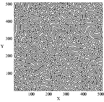
FIG. 1.: $\cos\kappa>0$ at $t=1000$ in a $512\times 512$ system.

This is a fairly early time for this system and we see that we have generated a set of local donuts. We have many concentric circles with few direct paths through the system. We clearly have layers but they are strongly bent.

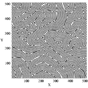
FIG. 2.: $\cos\kappa>0$ at $t=5000$ in a $512\times 512$ system.

When we reach a time of 5000 we see that most of the donuts have opened and stripes are forming and winding through the system. Clearly we see that the remaining centers of the donuts are serving as cores for large disclinations.

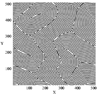
FIG. 3.: $\cos\kappa>0$ at $t=15000$ in a $512\times 512$ system.

This pattern coarsens as one moves to $t=15000$, as shown in Fig.3,

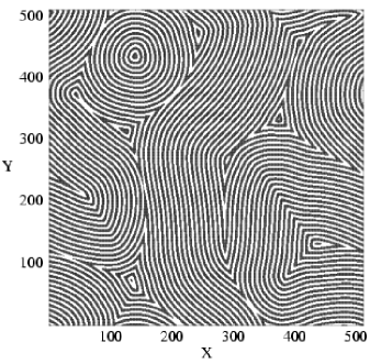
FIG. 4.: $\cos\kappa>0$ at $t=25000$ in a $512\times 512$ system.

and Fig. 4 where $t=25000$. In Fig. 4 one sees a target pattern in the upper left. One expects this to eventually break open.

These patterns can, at later times, be rather completely characterized by their defect structure. The defects can be found by looking for positions where the amplitude $Q^{2}$ is significantly smaller than its ordered value $Q_{0}^{2}=1$.

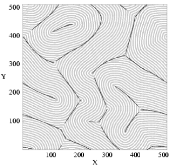
FIG. 5.: $\cos\kappa>0$ at $t=15000$ in a $512\times 512$ system. Those points with a small $Q^{2}$ are also shown.

In Fig. 5 we plot those points where $Q^{2}<0.5$ for the pattern in Fig. 3. We see that we have a rather complete map of the defect structure seen in the layer pattern. The small amplitude lines (SAL) network defines the pattern.

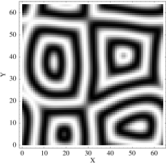
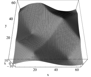
FIG. 6.: The pattern $\cos\kappa$ and $\kappa({\bf x})$ for a $64\times 64$ system at $t=800$.

In Fig. 6 we plot the pattern $\cos\kappa>0$ and $\kappa({\bf x})$ for a $64\times 64$ system at $t=800$. Clearly the peaks and anti-peaks correspond to the target centers of the pattern $\cos\kappa$, and the edges correspond to the SAL network. We also observe that the peaks and anti-peaks correspond to the $+1$ vortices in the ${\bf Q}$ field, and on some of the edges there is a $-1$ vortex of the ${\bf Q}$ field, as is shown in Fig. 7. The numbers of $+1$ and $-1$ vortices are equal, while the numbers of the peaks (anti-peaks) and the edges are usually not equal, so not every edge has a $-1$ vortex on it.

FIG. 7.: The ${\bf Q}$ field for the pattern in Fig. 6. The vector on each site is shown.

The $+1$ vortices are compact but the $-1$ vortices are not. This can be seen in Fig. 7, where some of the $-1$ vortices occupy entire edges. So the defects in the system are more like a domain-wall network rather than a set of vortices. The domain walls correspond to the edges in Fig. 6.

B Quantitative Results

At long times after a quench, phase ordering systems typically enter a scaling regime with a single characteristic length $L$. Here we check scaling for the correlation function $C_{\kappa}({\bf r},t)=\langle\kappa({\bf x}+{\bf r},t)\,\kappa({\bf x})\rangle$. In Fig. 8, we show this correlation function at 8 different times. The data is scaled so that we can see whether it obeys a scaling law. The correlation length can be extracted from $C_{\kappa}(r_{0},t)/C_{\kappa}(0,t)=1/2$ where $r_{0}\propto L$. The result is shown in Fig. 9. Since $|\nabla\kappa|\sim$constant, we expect that $\kappa\sim L$ and $\displaystyle C_{\kappa}(0,t)=\langle\kappa^{2}\rangle\sim L^{2}$. Thus we expect the scaling form $C_{\kappa}(r,t)=L^{2}\,F(r/L)$. The direct measurement of $\langle\kappa^{2}\rangle$ is shown in Fig. 10. From Fig. 9, we get $L\sim t^{0.60}$. From Fig. 10, we also obtain $L\sim t^{0.60}$.

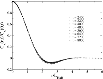
FIG. 8.: The correlation function $C_{\kappa}(r,t)$ for the $256\times 256$ system is plotted, for 8 different times, in scaling form. The distance $r$ is scaled by $L_{Half}=r_{0}$ given in Fig. 9. At least at small $r$, the function has a scaling form. The data is averaged over 41 runs.

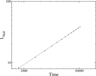
FIG. 9.: We extract the correlation length from $C_{\kappa}(r_{0},t)/C_{\kappa}(0,t)=1/2$. $r_{0}=L_{Half}$ is proportional to $L$. We find $L\sim t^{0.60}$. Averaged over 41 runs.

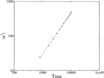
FIG. 10.: $\langle\kappa^{2}\rangle\propto t^{1.20}$. So $L^{2}\sim t^{1.20}$ and $L\sim t^{0.60}$. Averaged over 41 runs.

We measure next the number of defects in the system as a function of time after the quench. In Fig. 11 we plot the density of sites where $Q^{2}<0.4$ in the scaling regime. This curve is well fit by

$$n_{v}=a\,t^{-n}$$ (11)

with $a=3.89$, $n=0.506$. Since the total number of the defects is proportional to the area of domain walls, the number density is proportional to $w\cdot L/L^{2}=w\cdot L^{-1}$, where $w$ is the average width of the domain walls. Thus we estimate $L/w\sim 0.5$.

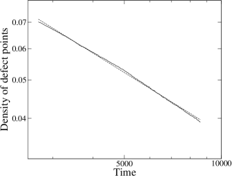
FIG. 11.: Density of the defect points where $Q^{2}<0.4$. Averaged over 38 runs.

It will turn out to be necessary to allow the width $w$ to be a function of time.

We need an independent method for determining $L$ or $w$. We do this by employing another method to measure the length of the defect network directly. Basically this is a coarse-graining method. We put the defect network on a lattice with lattice spacing $8\Delta r$ and count the number of sites it occupies. This number reflects the length of the network much better than the previous measurement. Other sizes of the lattice spacing can also be used as long as the grid size is larger than the width of the domain walls and much smaller than their lengths. The length density of the network is shown below and can be fit to $\sim t^{-0.60}$. Since the length density is proportional to $L/L^{2}=L^{-1}$, we get $L\sim t^{0.60}$, which is consistent with the measurement of the correlation function.

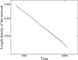
FIG. 12.: Length density of the defect points where the length of the network is in fact the number of sites that the network occupies in the lattice with larger grid. The dashed line is proportional to $t^{-0.60}$. Averaged over 38 runs.

We can then conclude that the average width of the domain walls $w\sim t^{0.10}$. In the time regime we study, the width $w$ is about $2\sim 4$. We don’t think $w$ will increase for ever, it may stop increasing at some later stage. But before that can happen in our system, finite size effect enters.

The growth laws for $L$ and $w$ can explain the growth exponents of other quantities. We give two examples below: $\langle Q^{2}\rangle$ and the energy density $\epsilon$ in Eq. (8).

The ordering of the field ${\bf Q}$ is characterized by the average over all sites of ${\bf Q}^{2}(i,j)$. We obtain the results shown in Fig. 13. It can be seen in the figure that there are two regimes where the data can be fit to a form

$$\langle Q^{2}\rangle=\frac{1}{a+bt^{-n}}~{}~{}~{}.$$ (12)

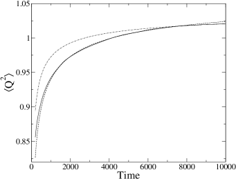
FIG. 13.: $\langle Q^{2}\rangle$ v.s. $t$. Averaged over 20 runs.

In the shorter time regime $1000\leq t\leq 7000$ the data is fit with with $a=0.930$, $b=3.15$, and $n=0.45$. In the longer time regime $7500\leq t\leq 10000$ we have the fit $a=0.950$, $b=2.40$, and $n=0.511$. In both fits the exponent $n$ is near $1/2$. We also see that in both fits the final value of $Q^{2}$ is larger than 1. Clearly more work needs to be done to establish the nature of this cross over. It seems likely that the final asymptotic value of $Q^{2}$ is greater than one due to finite size effects and the freezing of grain boundaries for long times.

In this system, $Q^{2}$ is approximately $1$ away from the domain-wall network and small on the domain walls with an average $c<1$. Because the average area $s$ of the domain walls in one domain is proportional to $wL$, and the domain’s area is $A\sim L^{2}$, we have

$$\langle Q^{2}\rangle=\frac{1}{A}\left[(A-s)\cdot 1+s\cdot c\right]=1-(1-c)\cdot\frac{s}{A}\ ,$$ (13)

where $s/A\propto wL^{-1}$. So the average of $Q^{2}$ has the form of $\langle Q^{2}\rangle-Q_{0}^{2}\sim w/L$. Thus we can identify $L/w\sim t^{0.5}$.

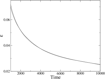
FIG. 14.: The energy density of the system. Averaged over 20 runs.

In Fig. 14 we show the path toward equilibration of the effective energy density $\epsilon$ defined by Eq.(9). This result seems to be in agreement with that for $Q^{2}$. We have a good fit to

$$\epsilon=a+bt^{-n}$$ (14)

with $a=0.0056$, $b=2.526$ and $n=0.5288$. Since the energy above the ground state should be proportional to the area of the domain walls, the energy density is proportional to $wL/L^{2}=wL^{-1}$. Again we get $L/w\sim t^{0.5}$.

IV Discussion

In the NLP model we know that there are analytic vortex solutions related to those for the XY model. This would seem to favor coarsening via a set of isolated vortices which pair up and annihilate. Instead we find large $-1$ vortices forming a domain wall network.

This system does not appear to generate dislocations and, as such, is quite different from the SH model which has a significant density of dislocations. The nonlinear phase model, on a larger scale, is growing targets and disclinations.

The NLP model introduced here helps to deepen our feeling that we do not have a good understanding of the general mechanism of stripe formation. In the SH model and the appropriate experiments the ordering is slow compared with the simple model of point defect annihilation. In this NLP model the ordering is “faster” than the simple model.

In this model we find two characteristic lengths, $L$ and $w$, which together explain the different exponents we observed. In the SH model, we also observed different exponents [8]. Our guess is that in SH model there are also more than one characteristic length.

In conclusion we see that models with the same symmetries can vary significantly in the defect structures produced during ordering. The search continues for models where one can dial the relative abundance of grain boundaries and free dislocations and disclinations. The ultimate goal is to match the models with a given experimental system.

Acknowledgments: This work was supported by the National Science Foundation under Contract No. DMR-0099324.

REFERENCES

- [1] K. R. Elder, J. Viñals, and M. Grant, Phys. Rev. Lett. 68, 3024 (1992).
- [2] M. C. Cross and D. I. Meiron, Phys. Rev. Lett. 75, 2152 (1995).
- [3] J. J. Christensen and A. J. Bray, Phys. Rev. E 58, 5364 (1998).
- [4] Q. Hou, S. Sasa, and N. Goldenfeld, Physica A 239, 219 (1997).
- [5] D. Boyer and J. Viñals, Phys. Rev. E 64, 050101 (2001).
- [6] D. Boyer and J. Viñals, Phys. Rev. E 63, 061704 (2001).
- [7] D. Boyer and J. Viñals, Phys. Rev. E 65, 046119 (2002).
- [8] H. Qian and G. F. Mazenko, Phys. Rev. E 67, 036102 (2003).
- [9] H. Qian and G. F. Mazenko, cond-mat/0304346.
- [10] C. Harrison, D. H. Adamson, Z. Cheng, J. M. Sebastian, S. Sethuraman, D. A. Huse, R. A. Register and P. M. Chaikin, Science 290, 1558 (2000).
- [11] J. Swift and P. C. Hohenberg, Phys. Rev. A 15, 319 (1977).
- [12] Y. Pomeau and P. Manneville, J. de Phsique – Lett., 40 (23), L-609 (1979).