A many-body interatomic potential for ionic systems: application to MgO

Abstract

An analytic representation of the short-range repulsion energy in ionic systems is described that allows for the fact that ions may change their size and shape depending on their environment. This function is extremely efficient to evaluate relative to previous methods of modeling the same physical effects. Using a well-defined parametrization procedure we have obtained parameter sets for this energy function that reproduce closely the density functional theory potential energy surface of bulk MgO. We show how excellent agreement can be obtained with experimental measurements of phonon frequencies and temperature and pressure dependences of the density by using this effective potential in conjunction with ab initio parametrization.

I Introduction

The problem of modelling the dynamics of ionic materials has a long historysangdix ; stoneham_and_harding . For many years the only available models were empirical force fields that were not very accurate or transferable between different environments. This was a problem both of the form of the model potentials used and the way in which these potentials were parametrized. Most frequently, simple pairwise effective potentials were used whose parameters were obtained using a combination of physical reasoning and empiricism. Such potentials could, at best, only be expected to produce qualitative or poorly-quantitative results.

The advent of ab initio molecular dynamicscarpar ; paynermp (MD) brought about a dramatic improvement in the accuracy with which the potential energy surface of the ions could be calculated, but this came with the price of an enormous increase in computational expense. In molecular dynamics simulations the precision with which thermodynamic properties can be calculated depends on the size of the system studied and the length of the simulation over which averages may be taken. For ab initio molecular dynamics one is generally confined to systems of around $100$ atoms and simulation times of $\sim 10$ picoseconds and so the precision with which many properties may be calculated is poor. In addition, for highly viscous liquids (such as silicatrave ; trave2 ) or very harmonic crystals the timescales available within ab initio MD may not be sufficient to adequately equilibrate the systemus_silica . Some ab initio-sized systems may suffer from finite size effects. For all these reasons there are many applications (good examples being the determination of melting temperatures or finite-temperature elastic constants) that are very difficult to tackle with ab initio MD and others (such as thermal conductivity and viscosity) that cannot be addressed at all.

Effective potentials are far less computationally expensive and so allow much longer simulation times and larger system sizes. It is therefore extremely desirable to find a compromise between the accuracy of ab initio MD and the computational speed of MD using effective potentials.

It has been shownfurio ; laio ; madden_mgo2 ; us_silica how the accuracy of an effective potential can be greatly improved by parametrizing using information from ab initio calculations. However in order for this to work a physically appropriate form for the potential must be used. Improving effective potentials therefore involves both using good parametrization procedures and appropriate forms for the potentials. The form that an effective potential takes should be flexible enough to describe the potential energy surface and specific enough to allow for efficient parametrization and application.

In this paper we present a many-body force field for ionic systems that incorporates the effect of an ion’s environment on its shape and size and the impact that such ionic distortions have on the short-range repulsive interactions between ions. These effects have been shown in the past to be important to the bonding of many simple ionic systemsschroder ; madden_compress ; madden_mgo1 . The force field presented has much in common with previously proposed “compressible-ion”madden_compress and “aspherical-ion”madden_mgo1 models but is superior from a computational point of view and avoids some problems associated with the way in which these models are implemented (see section III). It can also be implemented within a general mathematical framework that is very amenable to changes for the purposes of experimentation and improvement. A particularly attractive feature of the proposed force-field is that it can describe distortions of arbitrary shape. Previous models have been confined to describing distortions of certain given symmetries.

We apply the proposed model to crystalline and liquid magnesium oxide. MgO has been used in the past as a testing ground for models of ionic systemsmadden_compress ; madden_mgo1 . It is considered to be the simplest oxide and yet it is a system in which many-body interactions associated with distortions of the large oxide anion are known to be importantschroder ; boyer ; madden_compress . It is therefore a starting point for attempts to model the many body interactions in oxides and ionic systems in general.

MgO is a system of geophysical importance. It is an important component of the earth’s lower mantle and its stability up to high pressuresduffy make it useful as a pressure calibration standard for high pressure and temperature experiments. Since the vast majority of the compounds present in the earth’s mantle are oxides, MgO is a starting point for studies of the effects of pressure and temperature on mantle materials.

For MgO the use of our model is found to result in a significant improvement (over pairwise representations of the short-range repulsion) in the ability to fit the forces, stresses, and energies extracted from density functional theory (DFT)dft calculations. We use the model in conjunction with electrostatic interactions (involving both charges and induced dipoles) within a well-defined parametrization procedure. The resulting force field is shown to give a very good description of the structure and dynamics of MgO.

II Parametrizing a force field using ab initio data

As mentioned above, it has been shown for a number of systems that a very high level of accuracy may be achieved by parametrizing an effective potential by fitting to DFT forces, stresses, and energies in selected atomic configurationsfurio ; laio ; madden_mgo2 ; us_silica . However empiricism is also necessary unless one uses a functional form that is physically appropriate in the sense that it describes the electronic effects that are most important for the property one is studyingus_silica . In particular in reference us_silica, we have shown that, for silica, the inadequacy of simple pair potentials means that improving agreement with the forces and stresses from ab initio simulations, in general, disimproves the ability of empirically derived parameter sets to describe crystal structures. By inclusion of more many-body effects (in this case the polarizability of the oxygen anion) the ability of the force-field to reproduce ab initio data is improved and the empiricism becomes unnecessary for describing structure very accurately.

Here we make the assumption that ab initio calculations are highly accurate and always superior to calculations using effective potentials. This assumption is clearly formally unjustifiable but it is useful for our purposes. We aspire to ab initio accuracy and leave the improvement of the ab initio calculations themselves as a separate problem. We assume that if one achieves a perfect fit to ab initio data one gets an extremely accurate effective potential. However, as one moves away from this limit, the relationship between the fit to the ab initio data and the quality of the effective potential clearly weakens. If the fit is very poor then (as with the description of silica using pair potentialsus_silica ) even large improvements to it may not improve the ability of the potential to describe physical properties.

We define the fit as ${\bf\gamma}=(\Delta F,\Delta S,\Delta E)$, where $\Delta F$,$\Delta S$ and $\Delta E$ are dimensionless quantities corresponding to the averagesample percentage differences between forces, stress components, and energy differences between different configurations calculated ab initio and with the effective potential, i.e.

$$\Delta F = 100\times\frac{\sqrt{\sum_{k=1}^{n_{c}}\sum_{I=1}^{N}\sum_{\alpha}|F_{ep,I}^{\alpha}(\{\eta\})-F_{ai,I}^{\alpha}|^{2}}}{\sqrt{\sum_{k=1}^{n_{c}}\sum_{I=1}^{N}\sum_{\alpha}(F_{ai,I}^{\alpha})^{2}}}$$

$$\Delta S = 100\times\frac{\sqrt{\sum_{k=1}^{n_{c}}\sum_{\alpha,\beta}|S_{ep}^{\alpha\beta}(\{\eta\})-S_{ai}^{\alpha\beta}|^{2}}}{3B\sqrt{n_{c}}}$$

$$\Delta E = 100\times\frac{\sqrt{\sum_{k,l}^{n_{c}}((U^{k}_{ep}-U^{l}_{ep})-(U^{k}_{ai}-U^{l}_{ai}))^{2}}}{\sqrt{\sum_{k,l}^{n_{c}}(U^{k}_{ai}-U^{l}_{ai})^{2}}}$$

where $F^{\alpha}_{I}$ is the $\alpha^{\text{th}}$ cartesian component of the forces on ion $I$, $S^{\alpha\beta}$ denote stress components, $U^{k}$ is the potential energy of configuration $k$, $\{\eta\}$ is the set of parameters that, along with the functional form, characterise the effective potential. $B$ is a pressure that may be taken to be the bulk modulus of the material. The superscripts ’ep’ and ’ai’ indicate whether a quantity has been calculated with the effective potential or ab initio. In order for ${\bf\gamma}$ to be meaningful it is necessary that it be converged with respect to the number of configurations $n_{c}$ that have been used to test the effective potential. Typical values of $n_{c}$ are of the order of $10$.

Since our parametrization scheme does not discriminate between different contributions to the DFT forces, in order to be sure a priori that a potential works well one must have a very high quality fit to the ab initio data. This is because different properties depend to varying degrees on different contributions to the forces on the ions. It is difficult to know how a given value of, for example, $\Delta F$, manifests itself in the property that one is interested in studying. This is particularly true when there are a number of important contributions to the forces as these different contributions may be fit by an effective potential to varying degrees. If one has a potential that fits the ab initio forces perfectly then, clearly, each contribution is fit perfectly and this uncertainty is eliminated. For example, for silica the structure was extremely well described by using a good description of electrostatic effectsus_silica . However the forces differed from the ab initio ones by $\sim 16\%$. This suggests that the gross features of the potential energy surface are well described but that more local features and finer details, that are important for dynamics, may not be. We have observed that the diffusion of liquid silica at $3500$ K as described by the model proposed in reference  us_silica, seems to be too fast compared to extrapolations of lower temperature experimental datadiffusion . We also observe the phase transition between $\alpha-$ and $\beta-$cristobalite at too low a temperature. Both of these observations are consistent with an underestimation of local energy barriers due to a functional form that oversimplifies the short-ranged interactions between ions.

For every given functional form there are minimum values of $\Delta F$,$\Delta S$, and $\Delta E$ in parameter space. Functional forms that oversimplify the description of the electronic effects that are relevant for a given physical property may not be capable of achieving a close enough fit to the ab initio data to ensure that improvement of this fit improves the ability of the parameter set to describe physical properties. If this is the case then it is still conceivable that one may improve the agreement with experiment on many physical properties in an empirical way. We are of the opinion that an inability of a functional form to fit ab initio data indicates an intrinsic inadequacy of this form and that potentials created in this way should not be relied upon as being predictive. Effective potentials represent electronic effects in a phenomenological way. A potential that cannot produce very realistic values of the forces, stresses and energy differences must lack an important ingredient in its functional form and even if it produces good values for certain physical properties (such as those to which it was fit), for other properties it may show qualitatively different behaviour to the real system. A good potential form should fit the ab initio data to a high degree and significantly improving this fit should improve the property that one is interested in simulating. If this is the case then one can be confident that the ability to describe the property is due to a good microscopic description of the interatomic interactions.

Ultimately, our aim is to produce potentials that may be relied upon quantitatively to predict, not only the structures and the thermodynamic properties of bulk ionic systems, but also their dynamical properties. Although much work has been done in this direction (see, for example, references madden_mgo1, and madden_mgo2, and references therein) this is still a very ambitious goal. Finding a potential that describes dynamics well is a particularly difficult task angell .

However, the fact that DFT calculations can provide an essentially limitless amount of information that can be used in the parametrization process means that we are not constrained to using potential forms either with a small number of parameters or with parameters that have an obvious physical interpretation.

We use the same iterative parametrization scheme that was used in reference us_silica, . This is a slightly adapted form of the schemes used in references furio, and laio, and it allows us to make the very specific and non-trivial statement about a potential that for any atomic configuration created with the potential under specified thermodynamic conditions, the forces are, on average, within $p_{f}\%$ of those calculated ab initioabinitio , the stress components within $p_{s}\%$, and the energy-differences between configurations within $p_{e}\%$.

The parametrization scheme involves minimizing the function $\Gamma(\{\eta\})=\omega_{F}\Delta F+\omega_{S}\Delta S+\omega_{E}\Delta E$ with respect to the set of parameters $\{\eta\}$. In order to be sure that the minimization procedure is meaningful the number of ab initio configurations used in the fit ( $n_{c}$ ) is required to be reasonably large. In general its value depends on the system studied, the potential form used and the number of atoms in the unit cell. It was found that for MgO a value of $n_{c}=10$ was required in order to achieve convergence in the fit $\gamma$. In each step of the iteration at least a further five configurations were retained during the fitting procedure in order to test that the final functional form fit these configurations as well as it did those that were used in the minimization of $\Gamma(\{\eta\})$.

Minimization was performed using a combination of simulated annealingkirkpatrick and Powell minimizationnumerical_recipes . A basin in the surface defined by $\Gamma(\{\eta\})$ in $\eta-$space was initially found using simulated annealing and, once found, further minimization was performed using the method of Powell. Minimization of $\Gamma(\{\eta\})$using realistic force fields, and particularly simulated annealing, is a very computationally expensive process. However simulated annealing is very useful for two reasons : 1. It is very stable; Powell minimization can break down if numerical errors (such as overflow errors) occur due to unphysical values of the parameters; 2. In principle it can always bring one to the global minimum. In practice however this depends on how much computer time one is willing to allocate it. These properties of the simulated annealing method make it particularly useful when fitting a potential for the first time. One does not need to start with reasonable or physical values of the parameters in order for it to converge and this means that one may parametrize exotic potentials for which the parameters have no obvious physical interpretation.

The freedom that one is afforded using the combination of ab initio data and simulated annealing is crucial. It simply would not be possible to parametrize a force field such as the distortable-ion model introduced in section  IV without either one of these assets. If one depends on the use of experimental data, only force-fields containing a very small number of parameters may be parametrized if the fit is to be statistically significant. The amount of information that can be extracted from ab initio calculations is very large by comparison and so it allows much more complicated force-fields to be parametrized. If parametrization of a potential depends on good initial guesses for the parameters (as is the case with most optimization algorithms), each parameter must have an obvious physical interpretation and this can limit ones freedom when constructing a potential form. This problem can be solved by using simulated annealing in the parametrization process.

The ab initio calculations were performed with DFT within the local density approximationcepalder ; perzung using the planewave pseudopotential methodizc ; pickett . We have used soft norm-conserving pseudopotentialstm that are identical to those that have previously been used successfully to calculate its vibrational properties for a large range of pressures and temperatureskarki . We require our simulations to produce good quality forces and Karki et al. have performed much more rigorous tests of these pseudopotentials than it would have been feasible for us to perform. We perform our calculations on unit cells containing $64$ atoms under periodic boundary conditions and the Brillouin zone is sampled using only the $\Gamma-$point. A kinetic energy cutoff of $120$ Ryd. was used in the plane wave expansion of the wavefunctions in order to converge the stress very well.

III Many-body models for ionic systems

In this section a system for including many-body interactions in ionic systems will be introduced. We confine our attention to compounds in which variations in the degree of ionicity (either locally or globally) may be neglected. For such systems many body contributions to the interatomic interactions arise from the response of the size and shape of the ions to their environment. The anions carry multipole moments and, particularly the lowest order of these, the dipole moments, have an important impact on phonon spectra. The change in size and shape of the anions also has an impact on the short ranged Pauli exclusion repulsion between ions.

Although these effects are all interdependent, it has recently been shownmadden_pol ; madden_compress ; madden_mgo1 ; madden_mgo2 how an improved description of ionic dynamics may be achieved by independently incorporating them in the interatomic potential. Some of the ingredients of this force field have recently been parametrized using forces and stresses from density functional theory calculations and this resulted in an extremely good description of the potential energy surface in the crystalmadden_mgo2 .

The non-electrostatic repulsion between ions at short distances has in the past usually been modelled as an exponential function of the interionic distancesangdix ; bornmayer . The use of this exponential form rests on the assumptions that ions are spherical and of fixed size and that the repulsion between them due to the Pauli exclusion principle is proportional to the overlap between the ions whose charge distribution tails off exponentially. Although this may be an adequate approximation in crystals of high symmetry at low temperatures and a given pressure, at higher temperatures or at a different pressure or when a change of phase occurs, it is likely that anions will readjust their size and shape to fill the available space.

In order to cope with this, and in an attempt to improve the ability of ionic models to reproduce experimental equations of state and the relative energetics of different crystal structures, Wilson et al. have developed a compressible ion (CI) modelmadden_compress . Previously, ionic breathing effects had generally been incorporated within the shell modelschroder (for a recent application see reference matsui, ).

Wilson et al. wrote the potential energy due to short-range repulsive interactions between anion and cation as

$$V^{\text{sr}}_{+-}(\{R_{I}\};\{\delta\sigma_{I}\})=V_{\text{self}}(\{\delta\sigma_{I}\})+V_{\text{ov}}(\{R_{I}\};\{\delta\sigma_{I}\})$$ (1)

where $V_{\text{self}}$ is the sum of the changes in the internal energies of the ions and $V_{\text{ov}}$ is the total potential energy due to the repulsive overlap interaction between the ions, and $\delta\sigma_{I}$ is the change in the radius of ion $I$ from its average value $\overline{\sigma_{I}}$. From electronic structure calculations of the perfect cubic crystal it was found that $V_{\text{self}}$ could be written as

$$V_{\text{self}}(\{R_{I}\};\{\delta\sigma_{I}\})=\sum_{I\epsilon-}D_{I}\textrm{cosh}(\beta\delta\sigma_{I})$$ (2)

and the standard exponential form was adopted for the interaction energy :

$$V_{\text{ov}}(\{R_{I}\};\{\delta\sigma_{I}\})=\sum_{I\epsilon-,J\epsilon+}B_{IJ}e^{-\alpha_{IJ}(R_{IJ}-(\overline{\sigma_{I}}+\delta\sigma_{I}))}$$ (3)

At each timestep, during a simulation, the $\{\delta\sigma_{I}\}$ were required to take values that minimized $V^{\text{sr}}$.

Although this has been successful in reproducing some low temperature properties of MgO and CaO, such as the crystal energies as a function of volume, the prediction of phonon frequencies with this model was found to be quite poormadden_compress . This is because the distortion of the anions are in general not spherically symmetric if the crystal is disorderedmadden_compress ; madden_mgo1 . To account for aspherical distortions of the anion, Rowley et al.madden_mgo1 have extended the previous compressible-ion model by introducing eight further degrees of freedom to model distortions of dipolar and quadrupolar symmetry. Self-energy functions associated with these degrees of freedom were postulated.

With the aspherical-ion (AI) model and including dispersion effects and polarization effects, Rowley et al. managed to find parameters that gave good phonon dispersion curves for MgO. Very recently Aguado et al. have used an almost identical model, but with many of the parameters found from density functional theory calculations, to produce phonon dispersion curves and thermal expansion curves of a very high qualitymadden_mgo2 . Since thermal expansion depends on the second derivatives of the potential energy with respect to the ionic positions, this is a good test of this model’s representation of the potential energy surface of the crystal.

This method has the drawback that distortions of the anions are restricted to those of dipolar and quadrupolar symmetry. Although distortions of different symmetry could be incorporated, this would involve a large increase in the number of degrees of freedom and a corresponding decrease in the efficiency of the method. It would be desirable to include the effect of distortions of arbitrary shape in a way that is practicable.

In order to implement the above model in a computationally efficient way, an extended lagrangian approach has generally been used that is analogous to the Car-Parrinello methodcarpar for electronic structure theory. The degrees of freedom that describe ionic distortions ($\{\delta\sigma_{I}\}$ in the simple compressible-ion case) are the variables with which a “fictitious” dynamics was associated.

There are some problems associated with the use of a Car-Parrinello approach to modelling ionic distortions however:

• Recent workus_carpar has shown that, particularly for disordered systems, this method results in systematic errors in dynamics relative to methods in which the fictitious variables take their minimum energy values.

• The use of a small timestep is intrinsic to the extended lagrangian approach. For example, in the work of Aguado et al.madden_mgo2 a step of only $0.05$ femtoseconds was used. This is more than an order of magnitude smaller than the time step that can typically be used for non-Car-Parrinello approaches.

• The extended lagrangian approach is considerably more efficient during dynamics when variables are evolved from previous time steps than it is when minimizing the energy with respect to the extended variables for the first time. Since the parametrization process involves a large number of such minimizations, and is computationally very expensive, the extended lagrangian approach becomes much less efficient.

IV A Distortable Ion Model

Our goal is to develop a general mathematical framework within which the many-body effects of ionic compression and aspherical ionic distortion can be modelled, but that avoids the problems associated with the previously proposed models. In particular we would like to find a computationally efficient way of modelling these effects that avoids the use of an extended lagrangian and the introduction of fictitious degrees of freedom.

There are many open questions regarding the interactions between simple (electronically isolated) ions and so the framework should be general enough to allow for continual improvement of the specific form of the potential. For example, the form of the self-energy in equation 2 and the self energies associated with aspherical distortions can certainly be improved. It may also be worth investigating different forms of the overlap energy.

We will be primarily concerned with the anion-cation interaction. Of much lesser concern, initially at least, is the anion-anion interaction energy that has been found to provide only $\sim 3\%$ of the energetics of the perfect crystalmadden_mgo1 ; madden_compress . Although, the same cannot be said with any degree of certainty of more disordered phases, or systems of different stoichiometry such as SiO₂, it is nonetheless the most obvious place to start when constructing a potential.

We assume that a distortable ion ( such as O^2- ) has its shape and size “influenced” by all sufficiently close neighbouring ions. Much as in the scheme of Wilson, Madden and coworkersmadden_compress ; madden_mgo1 , an ion is described as a nucleus surrounded by a single membrane (representing the electrons) the radius of which is allowed to vary with the two polar angles (although in their case, the radius only varied in certain symmetric ways). The influence an ion $J$ exerts on ion $I$ can loosely be thought of as a restraining force on the ion’s tendency to expand and this restraint has a dependence on the polar angles $(\theta,\phi)$ in the spherical coordinate system centered on $I$. We also assume that the influence exerted at coordinates $(\theta,\phi)$ is zero if the angle between the outward unit vector at those coordinates ${\mathbf{\ell}}(\theta,\phi)$ and the vector ${\mathbf{R}}_{JI}={\mathbf{R}}_{J}-{\mathbf{R}}_{I}$ is greater than $90^{\circ}$.

We write the total influence on $I$ at $(\theta,\phi)$ due to all the other ions as

$$\rho_{I}^{(1)}(\theta,\phi)=\sum_{J\neq I}f_{IJ}(R_{IJ}){\mathbf{\ell}}(\theta,\phi)\cdot{\mathbf{x}}_{JI}\Theta({\mathbf{\ell}}(\theta,\phi)\cdot{\mathbf{x}}_{JI})$$ (4)

where ${\mathbf{x}}_{JI}={\mathbf{R}}_{JI}/R_{JI}$ and

$$\Theta({\mathbf{\ell}}(\theta,\phi)\cdot{\mathbf{x}}_{JI})=1\;\;\text{if}\;\;{\mathbf{\ell}}(\theta,\phi)\cdot{\mathbf{x}}_{JI}>0\\ \;\;\;\text{and}\;\;\;0\;\;\text{if}\;\;{\mathbf{\ell}}(\theta,\phi)\cdot{\mathbf{x}}_{JI}<0$$ (5)

Functional forms for $f_{IJ}(R)$ will be discussed in Section IV.A. The subscripts $IJ$ are to indicate that a different function is used for each distinct pair of ionic species.

Apart from a multiplicative constant, the spherical average of $\rho_{I}^{(1)}(\theta,\phi)$ is

$$\rho_{I}^{(0)}=\sum_{J\neq I}f_{IJ}(R_{IJ})$$ (6)

We write the angular dependent radius , $\sigma_{I}(\theta,\phi)$ of an ion as

$$\sigma_{I}(\theta,\phi)=\sigma_{I}^{(0)}(\rho^{(0)})+\sigma_{I}^{(1)}(\rho^{(0)},\rho_{I}^{(1)}(\theta,\phi))$$ (7)

In other words, the radius at $(\theta,\phi)$ is written as a sum of an average value due to the influence of all the ions and deviations from that average. Functional forms for $\sigma_{I}^{(0)}$ and $\sigma_{I}^{(1)}$ will be discussed in the next section. The distance between the membranes of ions $I$ and $J$ along their line of centers is

$$L_{IJ}=R_{IJ}-\sigma_{I}(\theta_{JI},\phi_{JI})-\sigma_{J}(\theta_{IJ},\phi_{IJ})$$ (8)

where $\theta_{JI}$ and $\phi_{JI}$ are defined such that ${\mathbf{\ell}}(\theta_{JI},\phi_{JI})={\mathbf{x}}_{JI}$. We will use the notation

$$\rho_{IJ}^{(1)} = \rho_{I}^{(1)}(\theta_{JI},\phi_{JI})$$ (9)

$$\sigma_{IJ}^{(1)} = \sigma_{I}^{(1)}(\rho^{(0)},\rho_{I}^{(1)}(\theta_{JI},\phi_{JI}))$$ (10)

$$\sigma_{IJ} = \sigma_{I}(\theta_{JI},\phi_{JI})$$ (11)

We now define the contribution to the total energy of the system from the short-range repulsive interactions as a sum of pairwise interactions between membranes.

$$U^{\text{\tiny SR}}=\sum_{I,J>I}U^{\text{\tiny SR}}_{IJ}(L_{IJ})g_{IJ}(R_{IJ})$$ (12)

where $g_{IJ}(R)$ takes the value $1$ for $R<R_{a}$, $0$ for $R>R_{b}$ and decays smoothly from $1$ to $0$ between $R_{a}$ and $R_{b}$. This allows us to truncate the interaction at intermediate distances.

The expression for the forces on the ions is given in Appendix A.

IV.1 Applying the model

In order to apply this model we clearly need to find suitable expressions for the functions $f_{IJ}$,$\sigma^{(0)}_{I}$, and $\sigma^{(1)}_{IJ}$. We begin by making the assumption that the most important interaction is the anion-cation interaction although this will be extended at a later stage to include the anion-anion interaction in a limited way. For the moment we are concerned with systems with two species such as MgO and we assume that the cation is small and rigid. For MgO it is likely that this is a very good assumption, given its degree of ionicity.

In order to draw a correspondence with the compressible ion model of Wilson et al.madden_compress (see section  III) we write the total energy of the system due to short-range repulsion as

$$V^{\text{SR}} = \sum_{I\epsilon-}V_{I}^{\text{self}}(\sigma_{I}^{(0)})+\sum_{I\epsilon-,J\epsilon+}B_{+-}e^{-\alpha_{-+}(R_{IJ}-\sigma^{(0)}_{I})}$$ (13)

$$+ \sum_{I,J\epsilon-,J>I}B_{--}e^{-\alpha_{--}R_{IJ}}+\sum_{I,J\epsilon+,J>I}B_{++}e^{-\alpha_{++}R_{IJ}}$$

The values of the anion radii at any time should be such that this repulsive energy is minimized. In other words

$$\frac{\partial V^{\text{SR}}}{\partial\sigma_{I}^{(0)}} = 0\;\;\;,\;\;\;\forall I$$ (14)

$$\Rightarrow\frac{\partial V_{I}^{\text{self}}}{\partial\sigma_{I}^{(0)}}+\alpha_{-+}e^{\alpha_{-+}\sigma_{I}^{(0)}}\sum_{J\epsilon+}B_{+-}e^{-\alpha_{-+}R_{IJ}} = 0$$ (15)

To simplify the notation we write $B^{\prime}=\alpha_{-+}B_{+-}$ and $\zeta(\sigma_{I}^{(0)})=\frac{\partial V^{\text{self}}}{\partial\sigma_{I}^{(0)}}$.

$$\zeta(\sigma_{I}^{(0)})e^{-\alpha_{-+}\sigma_{I}^{(0)}}=-\sum_{J\epsilon+}B^{\prime}e^{-\alpha_{-+}R_{IJ}}$$ (16)

As was noted previously in section IV there has been some discussion about the form of the self-energy of compressible ions. Although in the paper by Wilson et al.madden_compress the form used was that of a hyperbolic cosine of the amount of compression $\delta\sigma$, applications of the shell-model generally use a harmonic expression for this energy matsui ; schroder and in a very recent paper finnis Marks et al. have argued that for the oxide ion one should treat the $2p^{6}$ shell and the $s^{2}$ shells separately with harmonic and exponential compression energies respectively. In references madden_compress, and finnis, justification of the forms of $V_{\text{self}}$ used were based on quantum chemical calculations of the cold crystal under a large range pressures. The self-energy of ions in disordered systems may be quite different to that in the perfect crystal and anyway, for interatomic distances that one should expect to find in the crystal at zero pressure and temperatures up to the melting point, the calculated self-energy is still close to a linear regime. Furthermore we do not see any compelling physical reasoning behind any of the forms used. For these reasons we consider the form of this energy to be an open question. As a preliminary test of our model we have chosen an exponential form for $V_{\text{self}}$ as this simplifies the mathematics considerably. $\zeta(\sigma_{I}^{(0)})$ will then also have an exponential form so we may write

$$A_{I}e^{-\beta_{I}\sigma_{I}^{(0)}}e^{-\alpha_{-+}\sigma_{I}^{(0)}}=-\sum_{J\epsilon+}B^{\prime}e^{-\alpha_{-+}R_{IJ}}$$ (17)

By merging constant terms to simplify the notation, this equation can be rewritten in the form

$$\sigma_{I}^{(0)}(\rho_{I}^{(0)})=C_{1}+C_{2}\ln(\rho_{I}^{(0)})$$ (18)

where we say that

$$\rho_{I}^{(0)}=\sum_{J}C_{3}e^{-C_{4}R_{IJ}}$$ (19)

and $C_{1}$,$C_{2}$..etc are constants. By analogy with equation 6 we can say that

$$f_{IJ}=C_{3}e^{-C_{4}R_{IJ}}$$ (20)

One is not confined to such simple forms for the self-energy but for many forms one cannot write equation 16 in terms of $\sigma_{I}^{(0)}$ and one is forced to find $\sigma_{I}^{(0)}$ by an iterative procedure. This only has a very slight impact on the efficiency of calculating the potential. Another form that we have tried, and for which this procedure is used is

$$V_{I}^{\text{self}}(\sigma_{I}^{(0)})=\frac{\epsilon_{1}}{\epsilon_{2}+\sigma_{I}^{(0)}}+\frac{\epsilon_{3}}{(\epsilon_{4}+\sigma_{I}^{(0)})^{2}}$$ (21)

where $\epsilon_{1}$,$\epsilon_{2}$..etc are constants. This form was chosen according to the (admittedly, highly simplistic) physical reasoning that the internal factors that determine an ion’s radius are the electrostatic energy which varies like the inverse of a distance and the kinetic energy of the electrons which varies like the inverse of a distance squared.

The above analysis has shown that the distortable-ion model presented is mathematically equivalent to the compressible-ion model of Wilson et al. if $\sigma_{IJ}^{(1)}=0$ in the limit that the fictitious mass of the extended-lagrangian approach goes to zero.

It is not possible to map our approach onto the aspherical-ion model. However, we take a different approach to aspherical distortions. Given the functions $f_{IJ}$ and $\sigma^{(0)}_{I}$ as a starting point we may postulate a form for $\sigma_{IJ}^{(1)}$. We assume that the local distortion of an ion’s membrane scales with the local ”density” $\rho^{(1)}$ in the same way as the average radius scales with the spherical average of the density $\rho^{(0)}$. We therefore write

$$\sigma_{IJ}^{(1)}=C_{5}\ln\bigg{(}\frac{\rho_{IJ}^{(1)}}{\rho_{I}^{(0)}}\bigg{)}$$ (22)

Since we will be parametrizing this force by fitting to ab initio data, the minimization routine has the freedom either to make the constant $C_{5}$ very small or zero if this is not a reasonable functional form, or if aspherical distortions are really energetically equivalent to spherical ones it can make $C_{2}=C_{5}$ in which case the distortions of purely spherical symmetry disappear and

$$\sigma_{IJ}=C_{1}+C_{5}\ln(\rho_{IJ}^{(1)})$$ (23)

Although all the above derivation has assumed that this potential is only to be used for modelling cation-anion interactions, the generality and freedom afforded us by our parametrization procedure means that we lose nothing by trying to apply it to the anion-anion interaction also. We have done this by fitting parameters for the anion-anion interaction and we have found that it does improve the ability of the model to fit the ab initio forces. A more sensible, but also more expensive way of tackling the anion-anion interaction would be to introduce a self-consistent procedure to minimize the angular dependent radii simultaneously.

We also note that, as has been pointed out by Marks et al., different electronic shells have different compression characteristics. This could be modelled within the present scheme by having two or more such distortable ion potentials acting in parallel.

In our application of this model we have generally used timesteps of between $1$ fs and $1.5$ fs and the model has been found to be extremely efficient. As an example: in a simulation of $512$ atoms of crystalline MgO at $3300$ K (using potential F which is discussed in section IV.3) we have used a time step of $1$ fs. In this simulation, the time required for each calculation of the distortable-ion contribution to energy, forces, and stress was $0.57$ seconds on a single $300$Mhz SGI origin MIPS R12000 processor. On the other hand, the contribution of all the electrostatic terms was $3.0$ seconds. The total energy in this simulation drifted by approximately $2$ K per picosecond during this simulation. This energy drift can be almost eliminated by more fully converging the polarization at each time step.

A point to note regarding equation  4 is that there is a discontinuous change in $\Theta$ when ${\mathbf{\ell}}(\theta,\phi)\cdot{\mathbf{x}}_{JI}=0$. Although equation  4 itself is not discontinuous, its derivative with respect to the ionic positions is. This leads to discontinuous forces and consequently to a drift in the total energy. In practice we have not found this to be a problem as this drift in energy is very small compared to the drift that is due to the incomplete convergence of the polarization. However, if necessary this problem may be eliminated by replacing $\Theta$ with a function that varies smoothly from $1$ to $0$ as ${\mathbf{\ell}}\cdot{\mathbf{x}}_{JI}$ approaches zero.

IV.2 Testing the model

The model that we have proposed is considerably more complex than a pair potential and so in testing the model we first would like to verify that it improves upon simpler force fields. We confine ourselves to testing the usefulness of three different ingredients of the interionic potential:

1. A pairwise short-range interaction potential of the form

   $$U^{\text{\tiny SR}}_{IJ}(R_{IJ})=B_{IJ}e^{-\alpha_{IJ}R_{IJ}}-\frac{C_{IJ}}{R_{IJ}^{6}}-\frac{E_{IJ}}{R_{IJ}^{N_{IJ}}}$$ (24)

   where $B_{IJ},\alpha_{IJ},C_{IJ},E_{IJ},N_{IJ}$ are all parameters to be optimized.

2. A polarizable-ion potential including short-range polarization, as discussed in reference us_silica, . Only the oxygen ion is considered polarizable.

3. A distortable-ion potential, as discussed in sections IV and  IV.1. The interaction energy between ions $I$ and $J$ is given by

   $$U^{\text{\tiny SR}}_{IJ}(L_{IJ})=A_{IJ}e^{-\alpha_{IJ}L_{IJ}}+B_{IJ}e^{-\beta_{IJ}L_{IJ}}$$ (25)

   and the functions $f_{IJ}$,$\sigma^{(0)}_{I}$, and $\sigma^{(1)}_{IJ}$ are given the same forms as in equations 20, 18 and 22 respectively, i.e.

   $$f_{IJ}=C^{(1)}_{IJ}e^{-C^{(2)}_{IJ}R_{IJ}}$$ (26)

   $$\sigma_{I}^{(0)}(\rho_{I}^{(0)})=C^{(3)}_{I}\ln(\rho_{I}^{(0)})$$ (27)

   $$\sigma_{IJ}^{(1)}=C^{(4)}_{IJ}\ln\bigg{(}\frac{\rho_{IJ}^{(1)}}{\rho_{I}^{(0)}}\bigg{)}$$ (28)

   where $C_{1}$ from equation 22 has been merged into the pre-exponential factors $A_{IJ}$ and $B_{IJ}$. The parameters to be optimized are $A_{IJ}$, $\alpha_{IJ}$, $B_{IJ}$, $\beta_{IJ}$, $C^{(1)}_{IJ}$, $C^{(2)}_{IJ}$, $C^{(3)}_{I}$ ,$C^{(4)}_{IJ}$. The values $R_{a}=8.5$ a.u and $R_{b}=10$ a.u. were used in the decay function $g_{IJ}$.

In addition to the ingredients mentioned, each force field also included the point-charge electrostatic potential with the charge on an ion as a parameter.

We have parametrized five different force fields, as follows:

1. A pair-potential : short-range pair potential, parametrized in the crystal at ambient conditions.

2. A polarizable potential : short-range pair potential, with polarizable anions, parametrized in the crystal at ambient conditions.

3. A distortable-ion potential : distortable-ion potential, parametrized in the crystal at ambient conditions.

4. The full model : distortable-ion potential, with polarizable anions, parametrized in the crystal at ambient conditions.

5. The full model : distortable-ion potential, with polarizable anions, parametrized in the liquid at $3000$ K.

In order to avoid the computational expense of performing a full self-consistent parametrization procedure for each of these potentials we have only used this procedure to parametrize three potentials using the full model (distortable-ion model with point charges and dipole polarization). The three potentials were optimised at zero pressure for (i) the liquid at $3000$ K (ii) the crystal at $2000$ K and (iii) the crystal at $300$ K respectively. Each of these three potentials was used to create trajectories at the conditions for which it was optimised from which ’snapshot’ atomic configurations were extracted and used in ab initio calculations. We will show that the full model is the best at reproducing the ab initio data and so these configurations were considered to be as realistic as we have the ability to create.

Each of the potentials A to E was then parametrized using ab initio data from $10$ of these configurations (at the relevant conditions). Each potential thus created was then tested on its ability to fit $10$ new configurations (i.e. that were not used in the parametrization process) and also $10$ configurations at each of the other two sets of conditions. For example. potential A was parametrized at $300$ K and then its ability to fit the ab initio data in the crystal at $2000$ K and the liquid at $3000$ K was also tested. In all cases the error in the stress was evaluated relative to a pressure of $B=140$ GPa.

The results are summarized in table 1. We cannot guarantee that we have found the global minimum in each case during optimization as simulated annealing had to be done at a rather rapid quench rate. The simulated annealing was followed by Powell minimizationnumerical_recipes . In each case, the total minimization time was the same ($10$ days on a single processor) and therefore more economical force-fields are likely to be better minimized than less economical ones. A number of things can clearly be seen from table 1. First of all, not surprisingly, the distortable-ion model on its own is quite bad. This is probably because of the shortness of the range of its interactions. Ions further away from each other than $10$ a.u. interact only via the coulomb force between their charges. At $300$ K, the full model is clearly better than all other forms. It also transfers very well up to higher temperatures and to the liquid. The pair-potential, although working quite well for the crystal, does not transfer well to the liquid. The polarizable model yields results that are intermediate in quality between the pair-potential and the full model. The results are a clear illustration of the fact that by adding more physics into the form of an effective potential one can create force-fields with, not only an improved ability to fit the ab initio data, but also a much improved transferability between different phases and conditions.

The poor fit of potential E to the energy differences in the crystal at ambient conditions is because the energy differences in the liquid and high temperature solid are much greater than those at lower temperatures. The absolute value of the error in the energy differences is the same at low temperature and high temperature but $\Delta E$ is the error relative to the root-mean-squared value, which for the crystal is very small.

IV.2.1 Phonon Frequencies

Having established that our inclusion of many-body effects has improved the potential form with respect to the pair potential, at least according to the criterion that we have adopted, we now look at its ability to model the vibrational spectrum of MgO. We note once again that the DFT scheme to which the potential was fit gives a very good description of phonon frequencies at ambient conditions karki .

We find the phonon frequencies for our potential at a number of k-points from the positions of the peaks in the spectra of the spatial Fourier components of longitudinal and transverse charge and mass current correlation functionsquadrupole .

We performed an MD simulation on a system of $512$ atoms using the full-model, optimised in the crystal at $300$ K (potential D). The current correlation functions were calculated on a time domain of length $2.9$ ps that was averaged over a simulation of length $20$ ps. The phonon dispersions that we get are shown in figure 1. We get an extremely close fit to both the experimental and the self-consistent DFT data. The chief discrepancies are in the optical modes which are systematically underestimated. The longitunical optical mode in particular is underestimated near the zone center. Although we do not calculate the mode frequencies at $\Gamma=(0,0,0)$, as this would require an infinitely large simulation cell with the method that we are using, it looks as though the splitting between the longitudinal optical (LO) and the transverse optical (TO) phonons is slightly underestimated. In our parametrization procedure we have used a small cell to perform the ab initio calculations and so the long-range interactions that are important for dispersion near the $\Gamma-$point are not included. Our hope is that by modelling correctly the electrostatics at shorter range, we get a potential that, when used in a larger simulation cell, can accurately model the long range electrostatic interactions. This is not guaranteed however and is likely to work only if we include all relevant screening mechanisms in our functional form. The incorrect LO-TO phonon splitting suggests that our description of the electrostatics is incomplete since it arises from the long-range electric field induced by the LO phonon. This is not surprising since dipole polarization is only one of many screening mechanisms that are present in the real system. It may be that charge-transfer between ions is important. However, a comparison with the results of reference madden_mgo2, is suggestive of it being due to the fact that we haven’t included the affects of higher-order multipoles. Density functional perturbation theory calculationskarki of the Born effective charges yield values of $Z_{B}^{*}=\pm 1.94$. However, the charge on the oxygen ion in this potential (and all other potentials that we have fit) is $\sim 1.5$ - considerably less than this. Under the assumption that, within our model, short-range interactions and electrostatics describe completely separate aspects of the potential-energy surface (we do not know the extent to which this is true) the minimization routine fits the charge and the polarizability so as best to approximate the electrostatics of the crystal. The lack of higher order multipoles means that it must choose a compromise between purely dipole screening, in which the polarizability $\alpha$ and the charge $q$ take their “true” values, and uniform screening in which the charge is simply reduced by a factor equal to the dielectric constant and the polarizability is zero. In reference madden_mgo2, they use formal ionic charges and include both quadrupoles and dipoles and they get better agreement with experiment. Nevertheless, the description of the electrostatics that we have is significantly better than any other effective potential that we are aware of and quadrupoles would add considerably to the computational expense of the model.

It is also worth noting that, although in reference madden_mgo2, the potential used seems to give a slightly better description of the optical phonon frequencies, they report a fit to the DFT forces of $\Delta F<10\%$. Potential D is in significantly better agreement with our DFT data than this. Direct comparison of these two fits is not entirely justified, however. Aguado et al. fit to ab initio calculations of three different crystalline phases and therefore to three different coordination environments. Our fit of potential D is restricted to the phase and conditions at which we calculate the phonon frequencies. Although our fit is converged with respect to the number of atomic configurations tested, the small size of the fitting cell and the low temperature and high symmetry of these fitting conditions mean that only a very small region of phase space is visited. It may be that our functional form can numerically reproduce the potential energy surface in this small region of phase space in a way that is not necessarily physical and that therefore does not extend very well to describe the longer wavelength phonons that are present when we move to the larger simulation cell used for the calculation of phonon frequencies.

On the other hand, if one is to construct a potential for use in a given region of phase space it may not always be advisable to include configurations from regions of phase space that are too far away from this domain of application. There is a danger that changes in electronic structure that cannot be represented phenomenologically by the functional form of the potential may occur. For example, a change in coordination of the ions may be accompanied by a change in the degree of ionicity. Since our model keeps the charges on each ion fixed, by fitting to different coordination environments we may find charges that are the best compromise between the optimal values for each different environment, and that are therefore ideal for none of them. For many materials, the liquid structure is not too dissimilar to the solid at the same pressure and temperature and may therefore be a good compromise as a fitting environment. By fitting to the liquid we can visit a large volume of phase space that is nevertheless centered on or near the crystalline phase of interest.

We have used the above argument simply as a transparent way of discussing issues to consider when parametrizing a potential. The success of the potential created by Aguado et al. suggests that, for MgO, changes of ionicity do not present a problem in practice.

IV.3 Altering the model

The simple exponential form that we have used for the self energy was chosen for its simplicity. We would like to test other forms of this energy and although we do not go in detail into this problem here, we do parametrize a potential using the form of equation 21. This has an appealing physical form and it requires one to self-consistently find the values of the radii $\sigma^{(0)}_{I}$ and $\sigma^{(1)}_{IJ}$. We observed for the previously created potentials that changing the radial cutoffs for the decay function $g_{IJ}$ of the distortable ion model, $R_{a}$ and $R_{b}$, did not significantly change the fit to the ab initio. For larger distances the forces involved are either too small or cancel one another out. For this reason, and in order to improve efficiency we have used the slightly smaller values of $R_{a}=7.0$ a.u. and $R_{b}=8.0$ a.u.

Using the full model we perform a full self consistent parametrization in the liquid at $3000$ K (potential F) and the solid at $3000$ K (potential G). We have consistently found during our parametrizations that no significant improvement to the fit is obtained by including dispersion terms. It is likely that this is, at least partly, related to the limitations of the local density approximation as there is no reason to believe that it can describe such highly non-local dynamical fluctuations. Nevertheless, in the parametrization of potential F, $1/R^{6}$ and $1/R^{8}$ terms were used in conjunction with Tang-Toennies dispersion damping functionstangtoennies . The fact that the parametrization procedure made some of these interactions repulsive (see table LABEL:table:parameters_disp) is a clear indication that they should not necessarily be interpreted as representing the effect of electron dispersion.

We have then tested the ability of potentials F and G to fit ab initio data at these conditions. For this testing we use $20$ solid configurations and $20$ liquid configurations. The results are summmarized in table 2. The fit is extremely good and even better than that obtained with the previous form of the self-energy. However, a problem has been encountered with the potential that was parametrized on the solid at $3000$ K (potential G). We found that at higher temperatures and in the liquid, the iterative procedure by which the radii ($\sigma_{IJ}$) were found sometimes failed to converge. This is the explanation for the poor fit of potential G to the liquid data. This highlights the importance of caution when applying a force field to conditions different from those in which it was parametrized. During extensive simulations of the liquid the distortable ion model for the potential parametrized on the liquid never failed to converge.

The phonon dispersions for potential G are shown in figure 2. One should not expect results that are as good as those for a potential that is parametrized at ambient conditions, and so the results are extremely good. There is very good agreement with both experiment and the DFPT results of Karki et al.. As before, the worst agreement is for the long-wavelength LO phonons, and once again this is probably due to our incomplete description of electronic screening. It may also be that the very high symmetry of the relatively cold crystal makes polarization energetically unfavourable, and so the polarizability appropriate for a hot crystal is larger. A too-large polarizability should manifest itself in the phonon curves as a lowering of the energy of the long-wavelength LO phonon modes due to improved screening of the macroscopic electric field. Nevertheless, in general the results seem even better than those of figure 1 and the ability of both potentials to reproduce ab initio energy differences is very satisfying and suggests that the form of the distortable-ion self-energy used may be better than a simple exponential.

IV.3.1 Density

Figure 3 shows the equation of state of crystalline MgO at $300$ K for potentials D and G. Although both are in extremely good agreement with experiment at low pressures, potential D is better at much higher pressures. There are a number of possible reasons for this. First of all, although we should not expect our DFT calculations to produce exactly the same equation of state as that of Karki et alkarki due to differences in the details of the calculationseos , their equation of state does become increasingly inaccurate at high pressures. It may be that the improved fit of potential G to the ab initio data results in a disimprovement in the equation of state due to an inadequacy of the ab initio data. Another possibility is that the reduced values of $R_{a}$ and $R_{b}$ result in a reduction of transferability to high pressures due to the gradual introduction of more shells of neighbours in the distortable-ion calculation.

Figure 4 shows the density as a function of temperature for potentials F and G (Potential D gave very similar results to potential G for a system size of $512$ atoms). The experimentally observed thermal expansion is clearly very well reproduced by our potential. What is striking is that, particularly at low temperatures, finite size effects are very small. In reference madden_mgo2, finite size effects are much bigger. It may be that our model benefits from fitting the electrostatic interactions to the DFT data so that screening of interactions is more effective. It may also be that our potential over-screens the electrostatic interactions, i.e. that the dipole polarization is too large. This would be consistent with our underestimation of the LO mode frequencies approaching the $\Gamma$-point.

Our potentials overall give an extremely good description of the density as a function of pressure and temperature.

V Analysing the model

As discussed in section IV.1, we do not impose the distortable-ion model on the system. We have parametrized the force-field using simulated annealing that was begun at a high temperature. This means that, although we have supplied a functional form that is capable of including distortable-ion behaviour, the minimization routine is free to do with this form whatever is best for reproducing ab initio forces. The options that are open to the minimization routine are

• to disable all variable-radius functionality, and therefore to model the interionic forces with a double exponential of the interionic distance $R_{IJ}$. It would be optimal to do this if the way in which we model distortions is completely unphysical.

• to enable only the compressible-ion part of the model, i.e. that which is analogous to the model of Wilson et almadden_compress , thereby allowing only spherically symmetric anion distortions. It would be optimal for it to do this if the way in which we model aspherical distortions is unphysical but our description of spherical distortions is reasonable.

• to enable only the asymmetric part of the model and to disable purely spherically-symmetric distortions. This is optimal if our reasoning that aspherical distortions are energetically equivalent to spherical ones is true and the form of the model is reasonable.

• to partially enable either or both types of distortions as the best compromise between rigid-ion behaviour, breathing-ion behaviour and distortable-ion behaviour if all three of the models fail to varying degrees and in different ways to reproduce the ab initio potential energy surface.

The parametrization process is therefore itself a test of the distortable-ion model. We now look at what, precisely this parametrization process has done by examining the radius of an oxygen ion in the direction of a neighbouring magnesium ion for one of our potentials (potential F that is discussed in section IV.3). The test is performed in the crystal at $3000$K. The local radii of the anions consist of an arbitrary constant, that may be merged into the constant coefficient of the exponential force between ions, and the true variations of the radii due to changing environment. We look at the quantities $\sigma_{IJ}-\overline{\sigma_{IJ}}$ , $\sigma^{(1)}_{IJ}-\overline{\sigma^{(1)}_{IJ}}$, and $\sigma^{(0)}_{I}-\overline{\sigma^{(0)}_{I}}$ for anion $I$ and cation $J$ where $\overline{\sigma_{IJ}}$,$\overline{\sigma^{(1)}_{IJ}}$ and $\overline{\sigma^{(0)}_{I}}$ are averages over a long trajectory. These quantities are therefore the non-constant parts of the different contributions to the radius of ion $I$ in the direction of $J$ (Recall that $\sigma_{IJ}=\sigma^{(0)}_{I}+\sigma^{(1)}_{IJ}$ where $\sigma^{(0)}_{I}$ includes only spherically-symmetric distortions and $\sigma^{(1)}_{IJ}$ includes aspherical distortions ).

The results are shown in figure 5 and the variation in the value of $L_{IJ}$, as defined by equation 8, along the same trajectory is shown for comparison. As can be seen, the local radius is dominated by the effect of the aspherical part of the distortable-ion model. The spherical part makes a significantly smaller contribution. This clearly vindicates our extension of the compressible-ion model to include aspherical distortions.

The variation in the radius is very small compared to the variation in $L_{IJ}$ and so we look at what contribution this makes to the forces between the ions. Looking at the forces in a pairwise way is not entirely justified given the many-body nature of the potential, however it seems natural to look at the quantities

$$Q^{(1)}_{IJ}=100\times\frac{\frac{\partial U^{\text{\tiny SR}}_{IJ}(L_{IJ})}{\partial L_{IJ}}-\frac{\partial U^{\text{\tiny SR}}_{IJ}(R_{IJ}-\overline{\sigma_{IJ}}-\overline{\sigma_{JI}})}{\partial R_{IJ}}}{F^{\text{r.m.s.}}_{IJ}}$$ (29)

and

$$Q^{(2)}_{IJ}=100\times\frac{\frac{\partial U^{\text{\tiny SR}}_{IJ}(L_{IJ})}{\partial L_{IJ}}-\frac{\partial U^{\text{\tiny SR}}_{IJ}(R_{IJ}-\overline{\sigma_{IJ}}-\overline{\sigma_{JI}})}{\partial R_{IJ}}}{\frac{\partial U^{\text{\tiny SR}}_{IJ}(L_{IJ})}{\partial L_{IJ}}}$$ (30)

where $F^{\text{r.m.s.}}_{IJ}$ is the root mean-squared value (averaged over time) of the total force on anion $I$ (i.e. from all atoms and from both electrostatic and non-electrostatic contributions) projected onto the line joining the centers of $I$ and $J$. These quantities are plotted in figure 6. $Q^{(1)}$ is a way of looking at the impact of instantaneous variations of the membrane radii on the total force on the ion. $Q^{(2)}$ is a way of looking at the impact of instantaneous variations of the membrane radii on just the short-range part of the force between ions $I$ and $J$. If the radius of the ion is constant, then $Q^{(1)}=Q^{(2)}=0$. It is difficult to know how one should best compare forces, or judge the impact of individual contributions to the forces. However, inspection of these two quantities strongly suggests that, with the parameters of the model chosen by the minimization routine, the variation of the anion’s radius has a significant impact on dynamics.

The above discussion shows that the minimization routine finds it optimal to allow fully aspherical distortions of the anions that impact significantly on the interatomic forces.

VI Discussion

In this paper we have presented a many-body interatomic potential for ionic systems that attempts to model the effect on interionic interactions of ions breathing and distorting as their environments change. The potential has been used in conjunction with a rigorous ab initio parametrization scheme and applied to the case of bulk magnesium oxide. The only empiricism involved in our construction of these potentials has been in the choice of the form of the potential. We have justified this form by its ability to fit the density functional theory potential energy surface and to reproduce experimental data.

We have clearly shown that the form of the potential presented has a significantly improved ability (with respect to pairwise interactions) to fit the ionic potential energy surface of the hot crystal and the liquid calculated within density functional theory. It also has an improved transferability between phases and different physical conditions.

Once parametrized carefully, the potential has been shown to produce excellent phonon dispersion curves, equations of state and thermal expansion.

The computational expense of this potential is very small compared to other ingredients of realistic potentials such as dipole polarization. It is also likely to be much less expensive than previously proposed extended lagrangian force-fieldsmadden_compress ; madden_mgo1 , particularly since it allows the use of much larger timesteps.

For all these reasons, the potential proposed is a valuable addition to effective force fields that aim towards a quantitative description of real ionic materials.

The mathematical form of the potential is highly amenable to improvement and research into the optimal forms of its constituent functions may be expected to improve its ability to fit ab initio data.

Appendix A

Here we derive the expression for the forces on the ions from the definition of energy given in section IV

Using equations 8 and 12 the $\alpha$th force component on ion $K$ may be written as

$$F_{K}^{\alpha}= - \sum_{I,J>I}g_{IJ}\frac{\partial U^{\text{\tiny SR}}_{IJ}}{\partial L_{IJ}}\bigg{(}x_{IJ}^{\alpha}(\delta_{IK}-\delta_{JK})-\frac{\partial\sigma_{IJ}}{\partial R_{K}^{\alpha}}-\frac{\partial\sigma_{JI}}{\partial R_{K}^{\alpha}}\bigg{)}$$ (31)

$$- \sum_{I,J>I}U^{\text{\tiny SR}}_{IJ}\frac{\partial g_{IJ}}{\partial R_{IJ}}x_{IJ}^{\alpha}(\delta_{IK}-\delta_{JK})$$

and

$$\frac{\partial\sigma_{IJ}}{\partial R_{K}^{\alpha}} = \bigg{(}\frac{\partial\sigma_{I}^{(0)}}{\partial\rho_{I}^{(0)}}+\frac{\partial\sigma_{IJ}^{(1)}}{\partial\rho_{I}^{(0)}}\bigg{)}\frac{\partial\rho_{I}^{(0)}}{\partial R_{K}^{\alpha}}+\frac{\partial\sigma^{(1)}_{IJ}}{\partial\rho^{(1)}_{IJ}}\frac{\partial\rho_{IJ}^{(1)}}{\partial R_{K}^{\alpha}}$$ (32)

$$\frac{\partial\rho_{I}^{(0)}}{\partial R_{K}^{\alpha}} = \sum_{L(I)}\frac{\partial f_{IL}}{\partial R_{IL}}x^{\alpha}_{IL}(\delta_{IK}-\delta_{LK})$$ (33)

$$\frac{\partial\rho_{IJ}^{(1)}}{\partial R_{K}^{\alpha}} = \sum_{L(I)}\frac{1}{R_{LI}}(\delta_{LK}-\delta_{IK})(\delta^{\alpha\beta}-x_{LI}^{\beta}x_{LI}^{\alpha})x_{JI}^{\beta}f_{LI}A_{IJL}$$ (34)

$$+ \sum_{L(I)}\frac{1}{R_{JI}}(\delta_{JK}-\delta_{IK})(\delta^{\alpha\beta}-x_{JI}^{\beta}x_{JI}^{\alpha})x_{LI}^{\beta}f_{LI}A_{IJL}$$

$$+ \sum_{L(I)}x_{LI}^{\beta}x_{JI}^{\beta}\frac{\partial f_{LI}}{R_{LI}}x_{LI}^{\alpha}(\delta_{LK}-\delta_{IK})A_{IJL}$$

where $A_{IJK}=\Theta({\mathbf{x}}_{IJ}\cdot{\mathbf{x}}_{IK})$. The notation $\sum_{L(I)}$ has been introduced to indicate that the summation is over all ions $L$ that are neighbours of $I$. This is necessary for practical implementation due to the truncation of interactions and to avoid summing over all the particles.

Expanding equation 31 we get

$$F_{K}^{\alpha} = -\sum_{J(K)}U^{\text{\tiny SR}}_{KJ}\frac{\partial g_{KJ}}{R_{KJ}}x_{KJ}^{\alpha}$$ (35)

$$- \sum_{J(K)}\frac{\partial U^{\text{\tiny SR}}_{KJ}}{\partial L_{KJ}}g_{KJ}x_{KJ}^{\alpha}$$

$$+ \sum_{I(K)}\frac{\partial f_{KI}}{\partial R_{KI}}x_{KI}^{\alpha}\sum_{J(I)}\frac{\partial U^{\text{\tiny SR}}_{IJ}}{\partial L_{IJ}}g_{IJ}\bigg{(}\frac{\sigma^{(0)}_{I}}{\partial\rho_{I}^{(0)}}+\frac{\sigma_{IJ}^{(1)}}{\partial\rho_{I}^{(0)}}\bigg{)}$$

$$+ \Bigg{(}\sum_{J(K)}\frac{\partial U^{\text{\tiny SR}}_{KJ}}{\partial L_{KJ}}g_{KJ}\bigg{(}\frac{\sigma^{(0)}_{K}}{\partial\rho_{K}^{(0)}}+\frac{\sigma_{KJ}^{(1)}}{\partial\rho_{K}^{(0)}}\bigg{)}\Bigg{)}\Bigg{(}\sum_{I(K)}\frac{\partial f_{KI}}{\partial R_{KI}}x_{KI}^{\alpha}\Bigg{)}$$

$$- \sum_{I(K)}\frac{f_{KI}}{R_{KI}}\sum_{J(I)^{(1)}}\frac{\partial U^{\text{\tiny SR}}_{IJ}}{\partial L_{IJ}}g_{IJ}\frac{\partial\sigma_{IJ}^{(1)}}{\partial\rho_{IJ}^{(1)}}x_{IJ}^{\alpha}A_{IJK}$$

$$+ \sum_{I(K)}\frac{x_{KI}^{\alpha}}{R_{KI}}f_{KI}\sum_{J(I)}\frac{\partial U^{\text{\tiny SR}}_{IJ}}{\partial L_{IJ}}g_{IJ}\frac{\partial\sigma_{IJ}^{(1)}}{\partial\rho_{IJ}^{(1)}}x_{KI}^{\beta}x_{IJ}^{\beta}A_{IJK}$$

$$+ \sum_{I(K)}\frac{\partial U^{\text{\tiny SR}}_{KI}}{\partial L_{KI}}g_{KI}\frac{\partial\sigma_{KI}^{(1)}}{\partial\rho_{KI}^{(1)}}x_{KI}^{\alpha}\sum_{J(K)}\frac{f_{JK}}{R_{JK}}A_{KIJ}$$

$$- \sum_{I(K)}\frac{\partial U^{\text{\tiny SR}}_{KI}}{\partial L_{KI}}g_{KI}\frac{\partial\sigma_{KI}^{(1)}}{\partial\rho_{KI}^{(1)}}\sum_{J(K)}\frac{f_{JK}}{R_{JK}}x_{KJ}^{\beta}x_{KI}^{\beta}x_{KJ}^{\alpha}A_{KIJ}$$

$$- \sum_{I(K)}\frac{\partial U^{\text{\tiny SR}}_{KI}}{\partial L_{KI}}\frac{g_{KI}}{R_{KI}}\frac{\partial\sigma_{IK}^{(1)}}{\partial\rho_{IK}^{(1)}}\sum_{J(I)}x_{IJ}^{\alpha}f_{IJ}A_{IKJ}$$

$$+ \sum_{I(K)}\frac{\partial U^{\text{\tiny SR}}_{KI}}{\partial L_{KI}}g_{KI}\frac{\partial\sigma_{IK}^{(1)}}{\partial\rho_{IK}^{(1)}}\frac{x_{KI}^{\alpha}}{R_{KI}}\sum_{J(I)}x_{KI}^{\beta}x_{IJ}^{\beta}f_{IJ}A_{IKJ}$$

$$+ \sum_{I(K)}\frac{\partial U^{\text{\tiny SR}}_{KI}}{\partial L_{KI}}\frac{g_{KI}}{R_{KI}}\frac{\partial\sigma_{KI}^{(1)}}{\partial\rho_{KI}^{(1)}}\sum_{J(K)}x_{KJ}^{\alpha}f_{KJ}A_{KIJ}$$

$$- \sum_{I(K)}\frac{\partial U^{\text{\tiny SR}}_{KI}}{\partial L_{KI}}\frac{g_{KI}}{R_{KI}}\frac{\partial\sigma_{KI}^{(1)}}{\partial\rho_{KI}^{(1)}}x_{KI}^{\alpha}\sum_{J(K)}x_{KI}^{\beta}x_{KJ}^{\beta}f_{KJ}A_{KIJ}$$

$$- \sum_{I(K)}\frac{\partial f_{KI}}{\partial R_{KI}}x_{KI}^{\alpha}\sum_{J(I)}\frac{\partial\sigma_{IJ}^{(1)}}{\partial\rho_{IJ}^{(1)}}\frac{\partial U^{\text{\tiny SR}}_{IJ}}{\partial L_{IJ}}g_{IJ}x_{KI}^{\beta}x_{IJ}^{\beta}A_{IJK}$$

$$+ \sum_{I(K)}\frac{\partial U^{\text{\tiny SR}}_{KI}}{\partial L_{KI}}g_{KI}\frac{\partial\sigma_{KI}^{(1)}}{\partial\rho_{KI}^{(1)}}\sum_{J(K)}x_{KJ}^{\beta}x_{KI}^{\beta}x_{KJ}^{\alpha}\frac{\partial f_{KJ}}{\partial R_{KJ}}A_{KIJ}$$

In the derivation we have made the further assumptions that $f_{IJ}=f_{JI}$, $U^{\text{\tiny SR}}_{IJ}=U^{\text{\tiny SR}}_{JI}$ and $g_{IJ}=g_{JI}$.

TABLES

Table 1: The fit to the ab initio data for the different potential forms

	$300$K crystal			$2000$K crystal			$3000$K Liquid
	$\Delta F$	$\Delta S$	$\Delta E$	$\Delta F$	$\Delta S$	$\Delta E$	$\Delta F$	$\Delta S$	$\Delta E$
A	9.3	5.0	25.5	13.7	3.3	15.5	25.1	4.8	52.4
B	6.9	5.2	23.8	9.0	6.2	17.8	17.5	5.6	23.6
C	10.4	39.1	5.9	13.6	51.7	164.8	32.2	58.2	69.2
D	3.4	0.6	3.0	6.8	0.3	9.8	17.1	0.3	10.5
E	12.8	0.1	59.0	10.2	0.1	18.9	9.6	0.0	17.7

Table 2: The fit to the LDA ab initio data for the liquid (F) and solid (G) potentials used in the calculation of the melting slope.

	$3000$K Crystal			$3000$K Liquid
	$\Delta F$	$\Delta S$	$\Delta E$	$\Delta F$	$\Delta S$	$\Delta E$
F	9.6	0.1	10.8	10.4	0.2	10.2
G	6.2	0.3	10.6	44.0	2.3	54.0

Table 3: Parameters for potential F (atomic units)

Parameter	Mg-Mg	Mg-O	O-O
$b_{\text{pol}}$	-	$1.55713$	$4.01338$
$c_{\text{pol}}$	-	$-1.28035$	$31.93748$
$C^{(1)}$	-	$7.63066\times 10^{1}$	$1.58612\times 10^{3}$
$C^{(2)}$	-	$2.01709$	$2.42329$
$C^{(4)}$	-	$-4.09954\times 10^{-2}$	$2.248341\times 10^{-2}$
$A$	$4.10638\times 10^{12}$	$1.82404\times 10^{2}$	$-2.78524\times 10^{4}$
$\alpha$	$7.29702$	$2.22211$	$2.98764$
$B$	$-3.48800\times 10^{13}$	$-2.00799\times 10^{3}$	$4.00143\times 10^{3}$
$\beta$	$7.80852$	$3.71852$	$2.44883$

Parameter	Mg	O
$q$	$1.44831$	$-1.44831$
$\alpha$	-	$14.25305$
$C_{(3)}$	-	$-1.20698\times 10^{-2}$
$\epsilon_{1}$	-	$-1.44105\times 10^{7}$
$\epsilon_{2}$	-	$-5.14776$
$\epsilon_{3}$	-	$1.11436\times 10^{8}$
$\epsilon_{4}$	-	$7.20899$

Parameter	Mg-Mg	Mg-O	O-O
$C^{6}$	-	$-1.01505\times 10^{3}$	$3.24685\times 10^{4}$
$C^{8}$	-	$9.16150\times 10^{3}$ , $-6.70301\times 10^{6}$	$-5.93805\times 10^{6}$
$b_{\text{tt}}^{6}$	-	$2.51113\times 10^{-1}$	$-1.60446\times 10^{-1}$
$b_{\text{tt}}^{8}$	-	$3.78280\times 10^{-1}$ , $9.07552\times 10^{-2}$	$-7.45819\times 10^{-2}$

Table 4: Parameters for potential G (atomic units)

Parameter	Mg-Mg	Mg-O	O-O
$b_{\text{pol}}$	-	$1.65744$	$4.01338$
$c_{\text{pol}}$	-	$-1.35136$	$31.93748$
$C^{(1)}$	-	$1.00281$	$1.72179\times 10^{-5}$
$C^{(2)}$	-	$0.65944$	$0.19425$
$C^{(4)}$	-	$-3.18047\times 10^{-2}$	$-2.93661\times 10^{-2}$
$A$	$1.39895\times 10^{11}$	$2.16223\times 10^{2}$	$-5.03851\times 10^{4}$
$\alpha$	$6.72904$	$2.23873$	$3.09196$
$B$	$-2.50649\times 10^{13}$	$-4.21223\times 10^{2}$	$4.29645\times 10^{3}$
$\beta$	$7.98372$	$3.16438$	$2.43995$

Parameter	Mg	O
$q$	$1.48077$	$-1.48077$
$\alpha$	-	$10.40993$
$C_{(3)}$	-	$-1.33660\times 10^{-2}$
$\epsilon_{1}$	-	$-5.59871\times 10^{8}$
$\epsilon_{2}$	-	$7.61483\times 10^{-1}$
$\epsilon_{3}$	-	$4.89669\times 10^{8}$
$\epsilon_{4}$	-	$4.59914\times 10^{-1}$

Figures

Fig. 1 The phonon dispersions of MgO as calculated with the full polarizable and distortable-ion model parametrized in the crystal under ambient conditions (Potential D) compared with experimentsangster and with the density functional perturbation theory results of Karki et al.karki

Fig. 2 The phonon dispersions of MgO as calculated with the full polarizable and distortable-ion model parametrized in the crystal at $3000$K (Potential G) compared with experimentsangster and with the density functional perturbation theory results of Karki et al.karki

Fig. 3 The pressure of MgO as a function of density (at $300$ K) compared to experimentmao and density functional perturbation theory calculations karki . MD simulations used the full model potential parametrized at ambient conditions and simulation cells containing $512$ atoms.

Fig. 4 The density of MgO as a function of temperature (at zero pressure) compared to experimentthermal1 ; thermal2 for potentials G and F. Three different simulation cell sizes are used to check for finite size effects.

Fig. 5 a) $L_{IJ}-\overline{L_{IJ}}$ as a function of time, where $\overline{L_{IJ}}\approx 4.66$ a.u. is the average over the trajectory of $L_{IJ}$, the inter-membrane distance (see section IV). b) $\sigma_{IJ}-\overline{\sigma_{IJ}}$,$\sigma^{(1)}_{IJ}-\overline{\sigma^{(1)}_{IJ}}$, and $\sigma^{(0)}_{I}-\overline{\sigma^{(0)}_{I}}$. $I$ and $J$ are neighbouring anion and cation respectively.

Fig. 6 $Q^{(1)}_{IJ}$ and $Q^{(2)}_{IJ}$ (see equations 29 and 30)as a function of time along the same trajectory shown in figure 5

Figure 1:

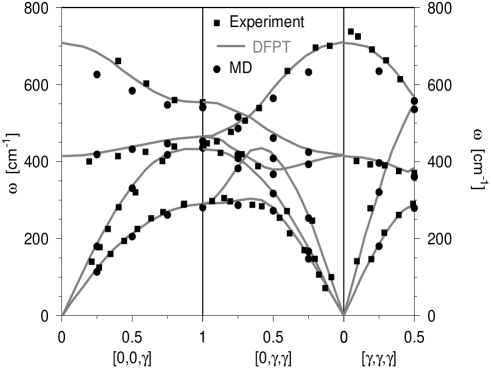
Figure 2:

Figure 3:

Figure 4:

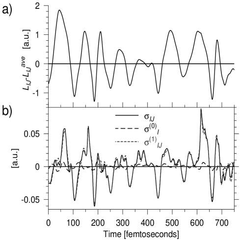
Figure 5:

Figure 6:

References

- (1) M. J. L. Sangster and M. Dixon Adv. Phys. 23, 247, (1976).
- (2) A. M. Stoneham and J. H. Harding, Annu. Rev. Phys. Chem. 37, 53 (1986).
- (3) R. Car and M. Parrinello, Phys. Rev. Lett. 55, 2471 (1985).
- (4) M. C. Payne, M. P. Teter, D. C. Allan, T. A. Arias, and J. D. Joannopoulos Rev. Mod. Phys. 64, 1045 (1992).
- (5) A. Trave, P. Tangney, S. Scandolo, A. Pasquarello, R. Car, Phys. Rev. Lett. 89, 245504 (2002).
- (6) A. Trave, Ph.D. Thesis, University of Geneva (2001).
- (7) P. Tangney and S. Scandolo, J. Chem. Phys. 117, 8898 (2002).
- (8) P. Tangney, Ph.D Thesis, SISSA, Trieste (2002).
- (9) F. Ercolessi and J.B Adams, Europhys. Lett. 26, 583 (1994)
- (10) A. Laio, S. Bernard , G. L. Chiarotti , S. Scandolo , E. Tosatti , Science 287, 1027 (2000) ; A. Laio, Ph.D Thesis, SISSA, Trieste (1999), available to download at : http://www.sissa.it/cm/thesis/1999/laio.ps.gz .
- (11) A. Aguado, L. Bernasconi and P. A. Madden Chem. Phys. Lett. 356, 437 (2002).
- (12) Averages are taken over a large number of sample configurations that have not been used in the optimization of parameters.
- (13) U. Schröder, Solid State Comm. 4, 347 (1966).
- (14) M. Wilson, P. A. Madden, N. C. Pyper, and J. H. Harding J. Chem. Phys. 104, 8068 (1996).
- (15) A. Rowley, P. Jemmer, M. Wilson and P. A. Madden J. Chem. Phys. 108, 10209 (1998).
- (16) L. L. Boyer, M. J. Mehl, J. L. Feldman, J. R. Hardy, J. W. Flocken, and C. Y. Fong Phys. Rev. Lett. 54, 1940 (1985).
- (17) T. S. Duffy, R. J. Hemley, and H.-K. Mao Phys. Rev. Lett. 74, 1371-1374 (1995).
- (18) P. Hohenberg and W. Kohn, Phys. Rev. 136, B864 (1964); W. Kohn and L. Sham, Phys. Rev. 140, A1133 (1965).
- (19) M. Hemmati and C.A. Angell, in “Physics Meets Mineralogy”, H. Aoki, Y. Syono, R.J. Hemley, eds. (Cambridge University Press, UK; 2000), p. 325.
- (20) G. Urbain, Y. Bottinga, and P. Richet, Geochim. Cosmochim. Acta 46, 1061 (1982).
- (21) This statement is true for an ab-initio calculation with specified approximations. Pseudopotentials, basis sets, sampling techniques and exchange-correlation functionals must all be specified.
- (22) S. Kirkpatrick, C. D. Gelatt, and M. P. Vecchi, Science, 220, 671-680, (1983).
- (23) W. H. Press, W. T. Vetterling, B. P. Flannery, and S. A. Teukolsky, Numerical Recipes in Fortran 77 and Fortran 90 : the art of scientific and parall el computing, 2nd Ed. , Camb. Univ. Press (1996).
- (24) D. M. Ceperley and B. J. Alder, Phys. Rev. Lett. 45, 566 (1980).
- (25) J. Perdew and A. Zunger, Phys. Rev. B 23, 5048 (1981).
- (26) J. Ihm, A. Zunger, and M. L. Cohen, J. Phys. C 4, 4409 (1979).
- (27) W. E. Pickett, Comp. Phys. Rep. 9, 115 (1989).
- (28) N. Trouiller and J. L. Martins, Phys. Rev. B 43, 1993 (1991)
- (29) B. B. Karki, R. M. Wentzcovitch, S. de Gironcoli and S. Baroni, Phys. Rev. B 61, 8793 (2000).
- (30) M. Wilson and P. A. Madden, J. Phys. : Condens. Matt. 5, 2687 (1993); 6, A151 (1994).
- (31) M. Born. and J. E. Mayer Z. Phys., 75, 1 (1932).
- (32) M. Matsui J. Chem. Phys.108, 3304 (1998).
- (33) P. Tangney and S. Scandolo, J. Chem. Phys. 116 , 14 (2002).
- (34) N. A. Marks, M. W. Finnis, J. H. Harding, and N. C. Pyper J. Chem. Phys. 114, 4406 (2001).
- (35) We use a much higher plane wave cutoff and this may become increasingly relevant at high pressures. We also sample the Brillouin zone in a different way.
- (36) D. Chandler, Introduction to Modern Statistical Mechanics, Oxford. Univ. Press. (1987), Chapter 8.
- (37) M. Wilson, B. J. Costa-Cabral and P. A. Madden , J. Phys. Chem. 100, 1227 (1996)
- (38) M. J. L. Sangster, J. Phys. Chem. Solids 34, 355 (1973).
- (39) K. T. Tang and J. P. Toennies J. Chem. Phys. 80, 3727 (1984).
- (40) C. S. Zha, H. K. Mao, R. J. Hemley, Proc. Nat. Acad. Sc. 97, 13494 (2000).
- (41) O. L. Anderson, K Zou, J. Phys. Chem. Ref. Data 19 69 (1990).
- (42) G. Fiquet, P. Richtet, G. Montagnac, Phys. Chem. Miner. 103, 27 (1999).