Local scale invariance and its application to strongly anisotropic critical phenomena

Malte Henkel^a, Alan Picone^a, Michel Pleimling^b and Jérémie Unterberger^c

^aLaboratoire de Physique des Matériaux and

Laboratoire Européen de Recherche Universitaire Sarre-Lorraine,

Université Henri Poincaré Nancy I, B.P. 239,

F – 54506 Vandœuvre lès Nancy Cedex, France

^bInstitut für Theoretische Physik I, Universität Erlangen-Nürnberg, D – 91058 Erlangen, Germany

^cInstitut Élie Cartan, Département de Mathématiques, Université Henri Poincaré Nancy I, B.P. 239,

F – 54506 Vandœuvre lès Nancy Cedex, France

The generalization of dynamical scaling to local scale invariance is reviewed. Starting from a recapitulation of the phenomenology of ageing phenomena, the generalization of dynamical scaling to local scale transformation for any given dynamical exponent $z$ is described and the two distinct types of local scale invariance are presented. The special case $z=2$ and the associated Ward identity of Schrödinger invariance is treated. Local scale invariance predicts the form of the two-point functions. Existing confirmations of these predictions for (I) the Lifshitz points in spin systems with competing interactions such as the ANNNI model and (II) non-equilibrium ageing phenomena as occur in the kinetic Ising model with Glauber dynamics are described.

1 Ageing and dynamical scaling

Non-equilibrium critical phenomena are a subject of intense research activity in physics. Rather than providing a general and exhaustive definition, we shall present a typical example of current interest, chosen such that our main question can be introduced in a natural way.

A common way to reach a situation of non-equilibrium criticality is through a rapid change of one of the macroscopic variables which enter into the equation of state. For definiteness, consider a simple ferromagnet. The simplest model system of this kind is the Ising model which considers magnetic moments attached to the sites of a (regular) lattice $\Lambda$. By hypothesis, these moments may only take two values, say ‘up’ and ‘down’, and are described through a spin variable $\sigma_{\boldsymbol{i}}=\pm 1$ attached to the lattice site $\boldsymbol{i}\in\Lambda$. In equilibrium, to a given configuration of spins $\{\sigma\}=\{\sigma_{\boldsymbol{i}}\}_{\boldsymbol{i}\in\Lambda}$ one associates an energy ${\cal H}\{\sigma\}=-\sum_{(\boldsymbol{i},\boldsymbol{j})}\sigma_{\boldsymbol{i}}\sigma_{\boldsymbol{j}}$ where the sum is usually restricted to nearest-neighbour pairs on the lattice. The probability of a given configuration $\{\sigma\}$ in equilibrium is then given by

$$P_{\rm eq}(\{\sigma\})=\frac{1}{Z}\exp\left(-{\cal H}\{\sigma\}/T\right)\;\;,\;\;Z:=\sum_{\{\sigma\}}\exp\left(-{\cal H}\{\sigma\}/T\right)$$ (1)

where $T$ is the temperature. It is well-known that systems of this kind show an order-disorder phase transition, at least in $d>1$ dimensions, such that the order parameter $\phi:=\langle\sum_{\boldsymbol{i}\in\Lambda}\sigma_{\boldsymbol{i}}\rangle$ has a non-vanishing value for temperatures below a certain critical temperature $T_{c}>0$ and vanishes for $T>T_{c}$. Such a model may be brought out of equilibrium, for example, by starting initially from a fully disordered state (effectively corresponding to an infinite temperature) and then quench the system rapidly to a fixed temperature below the system’s critical temperature $T_{c}>0$. Empirically, it is then found that the system evolves slowly towards the equilibrium state corresponding to the fixed temperature $T$. However, the details of this relaxation process may be complex. In many materials undergoing such thermal treatment, the time-dependent properties may well depend on the entire thermal history of the sample. The resulting ageing behaviour has been in the focus of intensive study, see [1, 2, 3, 4, 5] for reviews.

In the Ising model example, a popular choice to simulate the update of the individual spins is through Glauber dynamics [6]. Glauber dynamics may be realized through the discrete-time heat-bath rule $\sigma_{\boldsymbol{i}}(t)\to\sigma_{\boldsymbol{i}}(t+1)$ such that

$$\sigma_{\boldsymbol{i}}(t+1)=\pm 1\mbox{\rm~{}~{} with probability $\frac{1}{2}\left[1\pm\tanh(h_{\boldsymbol{i}}(t)/T)\right]$}$$ (2)

with the local field $h_{\boldsymbol{i}}(t)=\sum_{\boldsymbol{j}(\boldsymbol{i})}\sigma_{\boldsymbol{j}}(t)$, where $\boldsymbol{j}(\boldsymbol{i})$ runs over the nearest neighbours of the site $\boldsymbol{i}$. The main property of this dynamical rule is that the order parameter $\phi$ is not conserved. For non-equilibrium systems, there is no general theoretical framework for the calculation of the time-dependent probabilities $P(\{\sigma\};t)$. However, with the choice (2), $P(\{\sigma\};t)$ can be found exactly in $1D$ by solving an associated master equation [6]. The time-dependent spin-spin correlators and their approach towards equilibrium can be determined exactly in this special case. Otherwise, numerical simulation must be used.

    

Figure 1: Snapshots of the coarsening of ordered domains in the $2D$ Glauber-Ising model, after a quench to $T=1.5<T_{c}$ from a totally disordered state and at times $t=25$ (left) and $t=275$ (right) after the quench.

In figure 1, we illustrate the evolution of the microscopic state after a quench to $T<T_{c}$. We see that ordered domains form and slowly grow, with a typical size $L(t)\sim t^{1/z}$, where $z$ is the dynamical exponent. The presence of algebraic growth laws for such dynamic quantities, although the equilibrium state of the model is not critical, is characteristic for the ageing phenomena we wish to consider. Indeed, inside a given domain the spins are completely ordered and the time evolution of the model only occurs through the slow motion of the domain walls.

This evolution is more fully revealed through the study of two-time quantities, such as the two-time correlation function $C(t,s;\boldsymbol{r})$ and the (linear) autoresponse function $R(t,s;\boldsymbol{r})$

$$C(t,s;\boldsymbol{r})=\langle\phi(t,\boldsymbol{r})\phi(s,\boldsymbol{0})\rangle\;\;,\;\;R(t,s;\boldsymbol{r})=\left.\frac{\delta\langle\phi(t,\boldsymbol{r})\rangle}{\delta h(s,\boldsymbol{0})}\right|_{h=0}$$ (3)

where $\phi$ is the order parameter, $h$ the conjugate magnetic field, $t$ is called the observation time and $s$ the waiting time. Space translation invariance is assumed throughout. Autocorrelators are given by $C(t,s)=C(t,s;\boldsymbol{0})$ and autoresponses by $R(t,s)=R(t,s;\boldsymbol{0})$. One says that a system is ageing when $C(t,s)$ and/or $R(t,s)$ depend on both $t$ and $s$ and not only on their difference. Ageing phenomena are therefore related to a breaking of time-translation invariance. Physically, ageing occurs in the regime when $s$ and $\tau=t-s>0$ are simultaneously much larger than any microscopic time scale $\tau_{\rm micro}$. In many systems, one finds in the ageing regime a dynamical scaling behaviour, see [3, 4]

$$C(t,s)=s^{-b}f_{C}(t/s)\;\;,\;\;R(t,s)=s^{-1-a}f_{R}(t/s)$$ (4)

where $a$ and $b$ are non-equilibrium exponents. We emphasize that this non-equilibrium scaling also occurs for quenches exactly to the critical point $T=T_{c}$, but the values of the exponents found at $T=T_{c}$ will be different from those found for $T<T_{c}$. For $T<T_{c}$, it can be shown from phenomenological arguments that $z=2$ for dynamical rules with a non-conserved order parameter [8, 2], while at $T=T_{c}$, $z$ has a non-trivial value which must be determined from a full renormalization-group approach.

Table 1: Non-equilibrium exponents $a$ and $b$ for quenches from a fully disordered state onto and below the critical point $T_{c}>0$ of simple ferromagnets, according to [7].

	$a$	$b$	Class
$T=T_{c}$	$(d-2+\eta)/z$	$(d-2+\eta)/z$
$T<T_{c}$	$(d-2+\eta)/z$	0	L
	$1/z$	0	S

In table 1 we collect the values of the non-equilibrium exponents $a$ and $b$. Indeed, it turns out that for $T<T_{c}$ the equilibrium behaviour of the order parameter correlator is essential. If $C_{\rm eq}(\boldsymbol{r})\sim e^{-|\boldsymbol{r}|/\xi}$ with a finite $\xi$, we say that the system is of class S, while if $C_{\rm eq}(\boldsymbol{r})\sim|\boldsymbol{r}|^{-(d-2+\eta)}$, the system is said to be of class L, where $\eta$ is a standard equilibrium critical exponent. The results for $a$ are based on the well-accepted physical image that ageing comes from the slow motion of the domain walls [2, 3, 9]. This idea had been questioned recently and it was argued that because of some anomalous scaling behaviour, the simple relation $a=1/2$ should be invalid in the $2D$ Glauber-Ising model (which belongs to class S) and rather $a=1/4$ here [10]. However, recent tests have refuted this claim and reestablish that indeed $a=1/2$ in this model [7, 11].

The scaling functions are expected to behave for large arguments $x=t/s\gg 1$ asymptotically as

$$f_{C}(x)\sim x^{-\lambda_{C}/z}\;\;,\;\;f_{R}(x)\sim x^{-\lambda_{R}/z}$$ (5)

where $\lambda_{C}$ and $\lambda_{R}$ are called the autocorrelation exponent [12, 13] and autoresponse exponent [14], respectively. For a fully disordered initial state, it is traditionally accepted that $\lambda_{C}=\lambda_{R}=\lambda$. However, for spatially long-ranged initial correlations of the form $C_{\rm ini}(\boldsymbol{r})\sim|\boldsymbol{r}|^{-d-\alpha}$ (with $\alpha\leq 0$) the relation

$$\lambda_{C}=\lambda_{R}+\alpha$$ (6)

has been conjectured [14] and $\lambda_{C}=\lambda_{R}$ is only recovered if $\alpha$ renormalizes to zero. Furthermore, the rigorous arguments of [18] readily yield $\lambda_{C}\geq(d+\alpha)/2$, for simple ferromagnets without disorder. Very recently, distinct exponents $\lambda_{C}\neq\lambda_{R}$ have also been found in the random sine-Gordon model and in addition $\lambda_{C}<d/2$ violates the rigorous bound mentioned above [19].

Another central question in this context is whether/when under the conditions just described the system is in thermodynamic equilibrium. It is convenient to consider the fluctuation-dissipation ratio [20, 21]

$$X(t,s)=TR(t,s)\left(\frac{\partial C(t,s)}{\partial s}\right)^{-1}$$ (7)

At equilibrium, the fluctuation-dissipation theorem states that $X(t,s)=1$. The breaking of the fluctuation-dissipation theorem has been investigated intensively both theoretically (see e.g. [3, 4, 22, 23, 5, 24]) and experimentally [25, 26, 27].

Having thus reviewed the main phenomenological aspects of the ageing behaviour of simple ferromagnets, we can now formulate our main question: is it possible to generalize the dynamical scaling described by eq. (4) to a local scale invariance ? By this we mean that we wish to generalize the transformations of dynamical scaling $t\mapsto b^{z}t$ and $\boldsymbol{r}\mapsto b\boldsymbol{r}$ to a local form where $b=b(t,\boldsymbol{r})$ [28]. We therefore seek to extend dynamical scaling in a way analogous to the extension of global scale invariance in equilibrium critical phenomena to conformal invariance.

This review is organized as follows. In section 2 we present the main points of the construction of local scale transformations, for an arbitrary dynamical exponent $z$. In section 3 we consider in more detail the case $z=2$ where the relation to the conformal group and local Ward identities are discussed. In section 4, general expressions for the scaling functions of two-point functions are derived. Application to Lifshitz points are briefly discussed in section 5. Finally, in section 6 we return to applications of local scale invariance to ageing systems, focussing in particular on the prediction of the scaling of the response functions and tests in the Glauber-Ising model.

2 Construction of local scale transformations

We are interested in systems with strongly anisotropic or dynamical criticality. By definition, two-point functions of such systems satisfy the scaling form

$$G(t,\boldsymbol{r})=b^{2x}G(b^{\theta}t,b\boldsymbol{r})=t^{-2x/\theta}\Phi\left(rt^{-1/\theta}\right)=r^{-2x}\Omega\left(tr^{-\theta}\right)$$ (8)

where $t$ stands for ‘temporal’ and $\boldsymbol{r}$ for ‘spatial’ coordinates, $x$ is a scaling dimension, $\theta$ the anisotropy exponent (when $t$ corresponds to physical time, $\theta=z$ is called the dynamical exponent) and $\Phi,\Omega$ are scaling functions. Physical realizations of this are numerous, see [1, 2, 3, 5, 29] and references therein. For isotropic critical systems, $\theta=1$ and the ‘temporal’ variable $t$ becomes just another coordinate. It is well-known that in this case, scale invariance (8) with a constant rescaling factor $b$ can be replaced by the larger group of conformal transformations $b=b(t,\boldsymbol{r})$ such that angles are preserved. It turns out that in the case of one space and one time dimensions, conformal invariance becomes an important dynamical symmetry from which many physically relevant conclusions can be drawn [30].

Given the remarkable success of conformal invariance descriptions of equilibrium phase transitions, see e.g. [31, 32] for introductions, one may wonder whether similar extensions of scale invariance also exist when $\theta\neq 1$. Indeed, for $\theta=2$ the analogue of the conformal group is known to be the Schrödinger group [33, 34] (and apparently already known to Lie). We shall first describe the construction of these local scale transformations for arbitrary $\theta\neq 1,2$, show that they act as a dynamical symmetry, then derive the functions $\Phi,\Omega$ and finally comment upon some physical applications. We shall present the main results as formal propositions and refer to [28] for details and the proofs.

The defining axioms of our notion of local scale invariance from which our results will be derived are as follows (for simplicity, in $d=1$ space dimensions) [35, 28].

1. We seek space-time transformations with infinitesimal generators $X_{n}$, such that time undergoes a Möbius transformation

   $$t\to t^{\prime}=\frac{\alpha t+\beta}{\gamma t+\delta}\;\;;\;\;\alpha\delta-\beta\gamma=1$$ (9)

   and we require that even after the action on the space coordinates is included, the commutation relations $\left[X_{n},X_{m}\right]=(n-m)X_{n+m}$ remain valid. This is motivated from the fact that this condition is satisfied for both conformal and Schrödinger invariance.

2. The generator $X_{0}$ of scale transformations is $X_{0}=-t\partial_{t}-{\theta}^{-1}r\partial_{r}-{x}/{\theta}$ with a scaling dimension $x$. Similarly, the generator of time translations is $X_{-1}=-\partial_{t}$.

3. Spatial translation invariance is required.

4. Since the Schrödinger group acts on wave functions through a projective representation, generalizations thereof should be expected to occur in the general case. Such extra terms will be called mass terms. Similarly, extra terms coming from the scaling dimensions should be present.

5. The generators when applied to a two-point function should yield a finite number of independent conditions, i.e. of the form $X_{n}G=0$.

Proposition 1: Consider the generators

$$X_{n}=-t^{n+1}\partial_{t}-\sum_{k=0}^{n}\left(\mbox{${\begin{array}[]{c}n+1\\ k+1\end{array}}$}\right)A_{k0}r^{\theta k+1}t^{n-k}\partial_{r}-\sum_{k=0}^{n}\left(\mbox{${\begin{array}[]{c}n+1\\ k+1\end{array}}$}\right)B_{k0}r^{\theta k}t^{n-k}~{}~{}~{}$$ (10)

where the coefficients $A_{k0}$ and $B_{k0}$ are given by the recurrences $A_{n+1,0}=\theta A_{n0}A_{10}$, $B_{n+1,0}=\frac{\theta}{n-1}\left(nB_{n0}A_{10}-A_{n0}B_{10}\right)$ for $n\geq 2$ where $A_{00}=1/\theta$, $B_{00}=x/\theta$ and in addition one of the following conditions holds: (a) $A_{20}=\theta A_{10}^{2}$ (b) $A_{10}=A_{20}=0$ (c) $A_{20}=B_{20}=0$ (d) $A_{10}=B_{10}=0$. These are the most general linear first-order operators in $\partial_{t}$ and $\partial_{r}$ consistent with the above axioms 1. and 2. and which satisfy the commutation relations $[X_{n},X_{n^{\prime}}]=(n-n^{\prime})X_{n+n^{\prime}}$ for all $n,n^{\prime}\in\mathbb{Z}$.

Closed but lengthy expressions of the $X_{n}$ for all $n\in\mathbb{Z}$ are known [28]. In order to include space translations, we set $\theta=2/N$ and use the short-hand $X_{n}=-t^{n+1}\partial_{t}-a_{n}\partial_{r}-b_{n}$. We then define

$$Y_{m}=Y_{k-N/2}=-\frac{2}{N(k+1)}\left(\frac{\partial a_{k}(t,r)}{\partial r}\partial_{r}+\frac{\partial b_{k}(t,r)}{\partial r}\right)$$ (11)

where $m=-\frac{N}{2}+k$ and $k$ is an integer. Clearly, $Y_{-N/2}=-\partial_{r}$ generates space translations.

Proposition 2: The generators $X_{n}$ and $Y_{m}$ defined in eqs. (10,11) satisfy the commutation relations

$$\left[X_{n},X_{n^{\prime}}\right]=(n-n^{\prime})X_{n+n^{\prime}}\;\;,\;\;\left[X_{n},Y_{m}\right]=\left(n\frac{N}{2}-m\right)Y_{n+m}$$ (12)

in one of the following three cases: (i) $B_{10}$ arbitrary, $A_{10}=A_{20}=B_{20}=0$ and $N$ arbitrary. (ii) $B_{10}$ and $B_{20}$ arbitrary, $A_{10}=A_{20}=0$ and $N=1$. (iii) $A_{10}$ and $B_{10}$ arbitrary, $A_{20}=A_{10}^{2}$, $B_{20}=\frac{3}{2}A_{10}B_{10}$ and $N=2$.

In each case, the generators depend on two free parameters. The physical interpretation of the free constants $A_{10},A_{20},B_{10},B_{20}$ is still open. In the cases (ii) and (iii), the generators close into a Lie algebra, see [28] for details. For case (i), a closed Lie algebra exists if $B_{10}=0$.

Turning to the mass terms, we now restrict to the projective transformations in time, because we shall only need those in the applications later. It is enough to give merely the ‘special’ generator $X_{1}$ which reads for $B_{10}=0$ as follows [28]

$$X_{1}=-t^{2}\partial_{t}-Ntr\partial_{r}-Nxt-\alpha r^{2}\partial_{t}^{N-1}-\beta r^{2}\partial_{r}^{2(N-1)/N}-\gamma\partial_{r}^{2(N-1)/N}r^{2}~{}~{}~{}$$ (13)

where $\alpha,\beta,\gamma$ are free parameters (the cases (ii,iii) of Prop. 2 do not give anything new). Furthermore, it turns out that the relation $[X_{1},Y_{N/2}]=0$ for $N$ integer is only satisfied in one of the two cases (I) $\beta=\gamma=0$ which we call Type I and (II) $\alpha=0$ which we call Type II. The distinction between Type I and Type II is very important for the physical applications.

In both cases, all generators can be obtained by repeated commutators of $X_{-1}=-\partial_{t}$, $Y_{-N/2}=-\partial_{r}$ and $X_{1}$, using (12). Commutators between two generators $Y_{m}$ are non-trivial and in general only close on certain ‘physical’ states. One might call such a structure a weak Lie algebra.

Technically, these results depend on the construction of commuting fractional derivatives satisfying the rules

$$\partial_{r}^{a+b}=\partial_{r}^{a}\partial_{r}^{b}\;\;,\;\;\left[\partial_{r}^{a},r\right]=a\partial_{r}^{a-1}$$ (14)

The standard Riemann-Liouville fractional derivative is not commutative, see e.g. [36]. But if one uses the Hadamard definition of the Riemann-Liouville fractional derivatives, it is possible to generalize it by adding terms containing derivatives of the Dirac delta function. Then the relations (14) can be proven [28].

For $N=1$, the generators of both Type I and Type II reduce to those of the Schrödinger group. For $N=2$, Type I reproduces the well-known generators of $2D$ conformal invariance (without central charge) and Type II gives another infinite-dimensional group whose Lie algebra is isomorphic to the one of $2D$ conformal invariance [28]. The physical meaning of this new realization remains to be understood.

Dynamical symmetries can now be discussed as follows, by calculating the commutator of the generalized ‘Schrödinger-operator’ $\cal S$ with $X_{1}$. We take $d=1$ and $B_{10}=0$ for simplicity (it is trival that $\cal S$ commutes with the generators $X_{-1}=-\partial_{t}$ and $Y_{-N/2}=-\partial_{r}$ of time and space translations).

Proposition 3: The realization of Type I sends any solution $\psi(t,{r})$ with scaling dimension $x=1/2-(N-1)/N$ of the differential equation

$$\mathcal{S}\psi(t,\boldsymbol{r})=\left(-\alpha\partial_{t}^{N}+\left(\frac{N}{2}\right)^{2}{\partial}_{r}^{2}\right)\psi(t,{r})=0$$ (15)

into another solution of the same equation.

Proposition 4: The realization of Type II sends any solution $\psi(t,r)$ with scaling dimension $x=(\theta-1)/2+(2-\theta)\gamma/(\beta+\gamma)$ of the differential equation

$$\mathcal{S}\psi(t,r)=\left(-(\beta+\gamma)\partial_{t}+\frac{1}{\theta^{2}}\partial_{r}^{\theta}\right)\psi(t,r)=0$$ (16)

into another solution of the same equation.

In both cases, $\cal S$ is a Casimir operator of the ‘Galilei’-subalgebra generated from $X_{-1},Y_{-N/2}$ and the generalized Galilei-transformation $Y_{-N/2+1}$. The equations (15,16) can be seen as equations of motion of certain free field theories, where $x$ is the scaling dimension of that free field $\psi$. These free field theories are non-local, unless $N$ or $\theta$ are integers, respectively. Of course, the known dynamical symmetries of the free Schrödinger and Klein-Gordon equations are recovered for $N=1$ and $N=2$.

Phenomenological consequences will be discussed in section 4.

3 The case $z=2$ and the Schrödinger group

The origin of local scale invariance may be understood in more detail in the special case $z=2$. We consider the diffusion equation, in $d$ space dimensions

$$\left(2{\cal M}\partial_{t}-\boldsymbol{\partial}_{\boldsymbol{r}}\cdot\boldsymbol{\partial}_{\boldsymbol{r}}\right)\phi(t,\boldsymbol{r})=0$$ (17)

For fixed $\cal M$, the Schrödinger group is the maximal kinematic invariance group [33] on the space of solutions of eq. (17). It is defined by the space-time transformations ($\cal R$ is a rotation matrix and $\alpha,\beta,\gamma,\delta\in\mathbb{R}$)

$$t\longmapsto t^{\prime}=\frac{\alpha t+\beta}{\gamma t+\delta}\;\;,\;\;\boldsymbol{r}\longmapsto\boldsymbol{r}^{\prime}=\frac{{\cal R}\boldsymbol{r}+\boldsymbol{v}t+\boldsymbol{a}}{\gamma t+\delta}\;\;;\;\;\alpha\delta-\beta\gamma=1$$ (18)

and acts projectively on the solutions $\phi(t,\boldsymbol{r})$ [33]. We now present several new results on the diffusion equation and the Schrödinger group, again in the form of propositions. For details and the proofs we refer to [37].

Let $\mathfrak{sch}_{d}$ be the Lie algebra of (18) and $\mathfrak{conf}_{d}$ is the complexified Lie algebra of the conformal group in $d$ dimensions. Time-translations occur in $\mathfrak{sch}_{d}$ and are parameterized by $\beta$. We now treat the ‘mass’ $\cal M$ not as a constant but as another variable, see [38]. The wave function $\phi(t,\boldsymbol{r})$ which solves eq. (17) is replaced by $\psi=\psi(\zeta,t,\boldsymbol{r})$ through

$$\phi(t,\boldsymbol{r})=\frac{1}{\sqrt{2\pi}}\int_{\mathbb{R}}\!{\rm d}\zeta\,e^{-{\rm i}{\cal M}\zeta}\psi(\zeta,t,\boldsymbol{r})$$ (19)

which in turn satisfies the equation of motion

$$\left(2{\rm i}\frac{\partial^{2}}{\partial\zeta\partial t}+\frac{\partial^{2}}{\partial\boldsymbol{r}^{2}}\right)\psi(\zeta,t,\boldsymbol{r})=0$$ (20)

While $\mathfrak{sch}_{d}$ acts projectively on the wave functions $\phi(t,\boldsymbol{r})$ (the phase factor depends on $\cal M$), the action on $\psi(\zeta,t,\boldsymbol{r})$ is via a true representation. Furthermore, we have

Proposition 5: The Lie algebra of the maximal kinetic invariance group of equation (20) is $\mathfrak{conf}_{d+2}$. On the space of wave functions $\psi$ defined through eq. (19) one has the embedding

$$\mathfrak{sch}_{d}\subset\mathfrak{conf}_{d+2}$$ (21)

It is now of interest to study the subalgebras of $\mathfrak{conf}_{d+2}$. In particular, the parabolic subalgebras of $\mathfrak{conf}_{d+2}$ can be classified [37] and we obtain several new subalgebras, called $\widetilde{\mathfrak{age}}$ or $\widetilde{\mathfrak{alt}}$. For the case of one spatial dimension $d=1$, we illustrate in figure 2 their definition through the root space of $\mathfrak{conf}_{3}\cong B_{2}$. To each point of the diagram corresponds a generator of $\mathfrak{conf}_{3}$. For example, the generator of dilatations $X_{0}$ is one of the two generators sitting at the origin (the Cartan subalgebra $\mathfrak{h}$), the generator $X_{-1}$ of time translations has the coordinates $(-1,-1)$ and sits in the lower left corner of figure 2abc and the generator $Y_{-1/2}$ of space translations has the coordinates $(0,-1)$. Subalgebras of $\mathfrak{conf}_{3}$ are identified by considering all convex subset in this diagram.

Two of these parabolic subalgebras (figure 2bc) still contain the generator for the dilatations $t\to b^{2}t,\boldsymbol{r}\to b\boldsymbol{r}$ (which is in the Cartan subalgebra of $\mathfrak{conf}_{3}$) but do not contain time-translations anymore. In particular, $\widetilde{\mathfrak{age}}_{1}$ and $\widetilde{\mathfrak{alt}}_{1}$ are candidates for a dynamic symmetry algebra of ageing systems.

     

Figure 2: Root space of the complexified conformal Lie algebra $\mathfrak{conf}_{3}$, indicated by the full and the open points. The double circle in the center denotes the Cartan subalgebra. The generators belonging to the three non-isomorphic parabolic subalgebras [37] are indicated by the full points, namely (a) $\widetilde{\mathfrak{sch}}_{1}$, (b) $\widetilde{\mathfrak{age}}_{1}$ and (c) $\widetilde{\mathfrak{alt}}_{1}$.

While we have worked here in units such that the ‘speed of light’ $c=1$, it is possible to reintroduce $c$ explicitly into the equations of motion such as eq. (17). It had been claimed in the past that $\mathfrak{sch}_{d}$ could be obtained from a group contraction from $\mathfrak{conf}_{d+1}$ in the ‘non-relativistic limit’ $c\to\infty$ [39]. This limit procedure can be made precise in terms of the wave function (19) which satisfies a $(d+2)$-dimensional massless Klein-Gordon equation (20). We obtain the result

Proposition 6: The non-relativistic limit $c\to\infty$ of the conformal group acting on the wave function $\psi$ defined through (19) leads to the map

$$\mathfrak{conf}_{3}\to\widetilde{\mathfrak{alt}}_{1}$$ (22)

Although $\widetilde{\mathfrak{alt}}_{1}$ and $\widetilde{\mathfrak{sch}}_{1}$ have the same dimension, they are not isomorphic, see figure 2ac.

The dynamical symmetries of the free diffusion equation may be related to the symmetries of the action $S$ of the associated free-field theory. This action may be constructed in the standard fashion following the lines of Martin-Siggia-Rose theory, see e.g. [29] and references therein. Working with the wave function $\phi=\phi(t,\boldsymbol{r})$, we introduce a compound vector $\boldsymbol{\varepsilon}=(\delta t,\delta\boldsymbol{r})$ for small coordinate changes. Let $\eta$ be the phase which arises in the transformation of the wave function $\phi$ under local coordinate transformations. For local theories we expect the following transformation of the action

$$\delta S=\int\!{\rm d}t\,{\rm d}\boldsymbol{r}\>\left(T_{\mu\nu}\partial^{\mu}\boldsymbol{\varepsilon}^{\nu}+J_{\mu}\partial^{\mu}\eta\right)+\int_{t=0}\!{\rm d}\boldsymbol{r}\>\left(U_{\nu}\boldsymbol{\varepsilon}^{\nu}+V\eta\right)$$ (23)

where $T_{\mu\nu}$ is the conserved energy-momentum tensor and $J_{\mu}$ is the conserved probability current. The second term contains the contributions from the initial conditions. This local form permits the derivation of Ward identities and we obtain

Proposition 7: Consider an ageing system described by a local action $S$ transforming according to (23) and which is invariant under spatial translations, phase shifts, Galilei transformations and dilatations with $z=2$. Then $\delta S=0$ under the action of the special Schrödinger transformation $X_{1}$.

This illustrates the conceptual importance of the requirement of Galilei invariance, besides dynamical scaling with $z=2$, for full local scale invariance to hold. We stress that time-translation invariance is not required.

Finally, we mention that there exist infinite-dimensional Lie algebras which contain $\mathfrak{sch}_{d}$ as subalgebras. For example, the Schrödinger group (18) is a subgroup of the group defined by the transformations $t\to t^{\prime}$ and $\boldsymbol{r}\to\boldsymbol{r}^{\prime}$ where [37]

$$t^{\prime}=\beta(t)\;\;,\;\;\boldsymbol{r}^{\prime}=\boldsymbol{r}\sqrt{\dot{\beta}(t)\>}\;\;\mbox{\rm~{}~{} or else ~{}~{}}t^{\prime}=t\;\;,\;\;\boldsymbol{r}^{\prime}=\boldsymbol{r}-\boldsymbol{\alpha}(t)$$ (24)

and $\beta$ and $\boldsymbol{\alpha}$ are arbitrary functions. Whether this has a bearing on the non-equilibrium behaviour of spin systems is still open.

4 Scaling functions

From a physical point of view, the wave equations (15,16) discussed in section 2 suggest that the applications of Types I and II are very different. Indeed, eq. (15) is typical for equilibrium systems with a scaling anisotropy introduced through competing uniaxial interactions. Paradigmatic cases of this are so-called Lifshitz points which occur for example in magnetic systems when an ordered ferromagnetic, a disordered paramagnetic and an incommensurate phase meet (see [40] for a recent review). On the other hand, eq. (16) is reminiscent of a Langevin equation which may describe the temporal evolution of a physical system, with a dynamical exponent $z=\theta$. In any case, causality requirements can only be met by an evolution equation of first order in $\partial_{t}$.

We now give the scaling functions $\Phi,\Omega$ in eq. (8) from the assumption that the two-point function $G$ transforms covariantly under local scale transformations.

Proposition 8: [28] Local scale invariance implies that for Type I with $\theta=2/N$, the function $\Omega(v)$ must satisfy

$$\left(\alpha\partial_{v}^{N-1}-v^{2}\partial_{v}-Nx\right)\Omega(v)=0$$ (25)

together with the boundary conditions $\Omega(0)=\Omega_{0}$ and $\Omega(v)\sim\Omega_{\infty}v^{-Nx}$ for $v\to\infty$. For Type II, we have

$$\left(\partial_{u}+\theta(\beta+\gamma)u\partial_{u}^{2-z}+2\theta(2-z)\gamma\partial_{u}^{1-z}\right)\Phi(u)=0$$ (26)

with the boundary conditions $\Phi(0)=\Phi_{0}$ and $\Phi(u)\sim\Phi_{\infty}u^{-2x}$ for $u\to\infty$.

Here $\Omega_{0,\infty}$ and $\Phi_{0,\infty}$ are constants. The ratio $\beta/\gamma$ turns out to be universal and related to $x$. From the linear differential equations (25,26) the scaling functions $\Omega(v)$ and $\Phi(u)$ can be found explicitly using standard methods [28].

5 Application to Lifshitz points

Given these explicit results, the idea of local scale invariance can be tested in specific models. Indeed, the predictions for $\Omega(v)$ coming from Type I with $N=4$ nicely agree with cluster Monte Carlo data for the spin-spin and energy-energy correlators of the $3D$ ANNNI model at its Lifshitz point. The ANNNI model is defined in terms of Ising spins $\sigma=\pm 1$ on a hypercubic lattice. The Hamiltonian is

$${\cal H}=-\sum_{xyz}\sigma_{xyz}\left[\sigma_{xy(z+1)}+\sigma_{x(y+1)z}+\sigma_{(x+1)yz}\right]+\kappa\sum_{xyz}\sigma_{xyz}\sigma_{xy(z+2)}$$ (27)

where $\kappa$ is a constant. Extensive simulations using a generalization [41, 42] of the Wolff algorithm [43] and a new method [44] to reduce finite-size effects in the estimates of correlation functions led to a considerable improvement in the precision of the estimation of the location of the Lifshitz point, viz. $\kappa_{L}=0.270(4)$ and $T_{L}=3.7475(50)$ [41]. The Lifshitz-point exponents $\alpha_{L}=0.18(2),\beta_{L}=0.238(5),\gamma_{L}=1.36(3)$, respectively, of the specific heat, the magnetization and the susceptibility were obtained [41]. These values are also in good agreement with the results of a careful two-loop study of the $3D$ ANNNI model within renormalized field theory which gives $\alpha_{L}=0.160$, $\beta_{L}=0.220$ and $\gamma_{L}=1.399$ [45]. In figure 3, we show the scaling function $\Psi(v):=v^{\zeta}\Omega(v)$ of the spin-spin correlator. Here $\zeta=(2/\theta)(d_{\perp}+\theta)/(2+\gamma_{L}/\beta_{L})$, where $d_{\perp}=2$ is the number of transverse dimensions without competing terms and $\theta\simeq 1/2$ within the numerical accuracy of the data (see [41, 45, 28] for a fuller discussion of this point). We see the expected collapse of the data which establishes scaling. In the inset, we compare the data with the prediction of local scale invariance. If $\theta=2/N=1/2$, we have $N=4$ and expect from proposition 8 that $\Omega(v)$ satisfies

$$\alpha\frac{{\rm d}^{3}\Omega(v)}{{\rm d}v^{3}}-v^{2}\frac{{\rm d}\Omega(v)}{{\rm d}v}-4xv\Omega(v)=0$$ (28)

The are two independent solutions which satisfy the required boundary conditions, such that the form of $\Omega(v)$ depends on a single universal parameter $p$. Its value can in turn be estimated by considering universal ratios of moments of $\Omega(v)$, see [41] for details. In the inset of figure 3, we find perfect agreement with the prediction of local scale invariance.

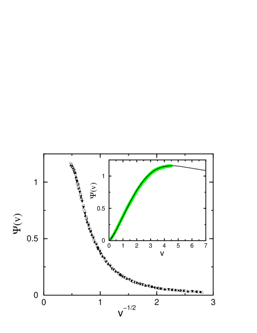
Figure 3: Scaling function $\Psi(v)$ of the spin-spin correlator at the Lifshitz point in the $3D$ ANNNI model. In the main plot the scaling of selected data for several values of $r_{\perp}$ is shown. In the inset, the full set of numerical data (gray points) is compared to the solution of eq. (28). The data are from [41].

Replacing the Ising model spins by so-called spherical spins $s_{\boldsymbol{r}}\in\mathbb{R}$ such that $\sum_{\boldsymbol{r}\in\Lambda}s_{\boldsymbol{r}}^{2}={\cal N}$, where $\cal N$ is the number of sites of the lattice, one obtains the exactly solvable ANNNS model. At its Lifshitz point, the spin-spin correlator agrees exactly with the prediction of local scale invariance [46, 35, 28].

On the other hand, the predictions of Type II have been tested extensively in the context of ageing ferromagnetic spin systems which are going to be described in the next section.

6 Application to ageing

Time translation invariance does not hold in ageing systems. The simplest way to do this is to remark that the Type II-subalgebra spanned by $X_{0},X_{1}$ and the $Y_{m}$ leaves the initial line $t=0$ invariant, see (13). Therefore the autoresponse function $R(t,s)$ is fixed by the two covariance conditions $X_{0}R=X_{1}R=0$. Solving these differential equations leads to

Proposition 9: [47, 28] For a statistical non-equilibrium system which satisfies local scale invariance the autoresponse function $R(t,s)$ takes the form

$$R(t,s)=r_{0}\left(t/s\right)^{1+a-\lambda_{R}/z}\left(t-s\right)^{-1-a}\;\;,\;\;t>s~{}~{}~{}~{}$$ (29)

where $a$ and $\lambda_{R}/z$ are the non-equilibrium exponents defined in section 1 and $r_{0}$ is a normalization constant.

The functional form of $R$ is completely fixed once the exponents $a$ and $\lambda_{R}/z$ are known. Similarly, $R(t,s;\boldsymbol{r})=R(t,s)\Phi\left(r(t-s)^{-1/z}\right)$ gives the spatio-temporal response, with the scaling function $\Phi(u)$ determined by (26) [28]. In the $z=2$ special case the above result takes a particularly simple form.

Proposition 10: [48, 37] For an ageing system with dynamical exponent $z=2$ and which is invariant under $\mathfrak{age}_{d}$, the two-time spatio-temporal response function is

$$R(t,s;\boldsymbol{r})=R(t,s)\exp\left[-\frac{\cal M}{2}\frac{\boldsymbol{r}^{2}}{(t-s)}\right]$$ (30)

where $R(t,s)$ is given by eq. (29).

The form of the two-point function does not change if we use $\mathfrak{alt}_{d}$ instead.

Ageing systems are often described in terms of Langevin equations of the form

$$\dot{\phi}(t)=-\frac{\delta{\cal H}}{\delta\phi(t)}+\eta(t)$$ (31)

where $\eta(t)$ is assumed to be a Gaussian noise with mean zero and variance $\langle\eta(t)\eta(t^{\prime})\rangle=2T\delta(t-t^{\prime})$. In the context of Martin-Siggia-Rose theory, it can be shown that response functions can be written as a correlator $R(t,s)=\langle\phi(t)\widetilde{\phi}(s)\rangle$ of the order parameter $\phi$ and its associated response field $\widetilde{\phi}$. On the other hand, to each solution $\phi(t,\boldsymbol{r})$ with positive mass ${\cal M}>0$ there exists a conjugate solution $\phi^{*}(t,\boldsymbol{r})$ which satisfies the diffusion equation with $\cal M$ replaced by $-{\cal M}$ and which can be said to have negative mass.

On the other hand, if we work instead with the wave function $\psi(\zeta,t,\boldsymbol{r})$ as defined in eq. (19), we can use the embedding $\mathfrak{sch}_{d}\subset\mathfrak{conf}_{d+2}$ and the form of the two- and three-point functions is fixed by conformal invariance. For ageing systems, time-translation invariance does not hold and we must restrict to those parabolic subalgebras which do not contain $X_{-1}$. We are interested in the linear response functions

$$R_{2}(t_{1},s) = \frac{\delta\langle\phi(t_{1})\rangle}{\delta h(s)}=\langle\phi(t_{1})\widetilde{\phi}(s)\rangle$$ (32)

$$R_{3}(t_{1},t_{2},s) = \frac{\delta\langle\phi(t_{1})\phi(t_{2})\rangle}{\delta h(s)}=\langle\phi(t_{1})\phi(t_{2})\widetilde{\phi}(s)\rangle$$ (33)

Instead, we may also calculate them using the functions $\psi(\zeta,t,\boldsymbol{r})$ and then find

Proposition 11: [37] For an ageing system with $z=2$ and which is invariant under $\mathfrak{age}_{d}$, the two- and three-time spatio-temporal response functions may be obtained from

$$R_{2}(t_{1},s) = \langle\phi(t_{1})\phi^{*}(s)\rangle$$ (34)

$$R_{3}(t_{1},t_{2},s) = \langle\phi(t_{1})\phi(t_{2})\phi^{*}(s)\rangle\;\;$$ (35)

such that the causality conditions $t_{1}>s$ and $t_{2}>s$ are automatically satisfied.

This suggests the identification of the response field

$$\widetilde{\phi}=\phi^{*}$$ (36)

with the conjugate solution of the Schrödinger equation. Explicit expressions for these response functions are known.

Finally, Galilei invariance holds de rigueur only for a vanishing temperature $T=0$ and in principle all predictions made on ageing systems so far are restricted to that case. However, constructing the free-field Martin-Siggia-Rose action it can be seen through the Wick theorem that the perturbative series in $T$ terminates after the first term.

Proposition 12: [49] For an ageing Gaussian system with $z=2$ and which is invariant under $\mathfrak{age}_{d}$ and at a temperature $T<T_{c}$, the response function $R(t,s)$ agrees to all orders in $T$ with eq. (29).

This argument is expected to work in the low-temperature phase, where $T$ flows to zero under the action of the renormalization group [2] so that perturbation theory should be applicable. Direct evidence in favour of this is given below. The independence of the form of $R(t,s)$ on the (short-ranged) initial conditions is all the more remarkable since for instance the correlators do depend on them [49]. On the other hand, at $T=T_{c}$ thermal fluctuations and fluctuations of the initial state become simultaneously important. Remarkably enough, there exists good numerical evidence that eq. (29) even holds at $T=T_{c}$ in the $2D$ and $3D$ Glauber-Ising model [47]. However, a two-loop renormalization group calculation of the O($n$) field theory gives a numerically small correction to eq. (29) [50]. The understanding of the rôle of temperature on the validity of Galilei invariance in field theory will require more work.

A quantitative test of the prediction (29) is best carried out through the consideration of an integrated response function, such as the thermoremanent magnetization

$$M_{\rm TRM}(t,s)=h\int_{0}^{s}\!{\rm d}u\,R(t,u)=r_{0}\,s^{-a}f_{M}(t/s)$$ (37)

where the system is quenched in a small (random [51]) magnetic field $h$ which is turned off after the waiting time $s$ has elapsed. The magnetization is then measured at a later time $t$. Local scale invariance furnishes, via (29), an explicit predictions for the scaling function $f_{M}(x)$. In certain cases there may be sizeable correction terms to this scaling form, see [7, 10, 11, 52, 53] for details.

   

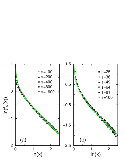
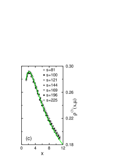
Figure 4: Scaling form of the integrated magnetic response in the Glauber-Ising model as a function of $x=t/s$ below criticality. The symbols correspond to different waiting times $s$. The integrated autoresponse is shown (a) in $2D$ at $T=1.5$ and (b) in $3D$ at $T=3$. An example of the integrated spatio-temporal response in $2D$ at $T=1.5$ and with $\mu=2$ is shown in (c). The full curves are obtained from (29). After [52].

We now consider ageing in the Glauber-Ising model (2), quenched to a temperature $T<T_{c}$ from a fully disordered initial state. Then the exponents $a=1/z=1/2$ and $\lambda_{R}\simeq 1.26$ and $1.6$ in $2D$ and $3D$, respectively, are known. In figure 4ab, the scaling function $f_{M}(x)$, as obtained from large-scale simulations, is shown for several values of the waiting time $s$. In both two and three dimensions, a nice scaling behaviour is found and the form of the scaling function agrees very well with the prediction from eq. (29).

For $z=2$, we have seen in section 3 the importance of Galilei invariance as the second building block, besides dynamical scaling, of the local scale invariance of systems whose action $S$ transforms according to eq. (23). It is therefore important to test Galilei invariance directly, which can be done by considering the spatio-temporal response $R(t,s;\boldsymbol{r})$ and testing it for the form eq. (30) [52]. We first fix the mass $\cal M$ by studying how the integrated response $\int_{0}^{s}\!{\rm d}u\,R(t,u;\boldsymbol{r})$ depends on $r^{2}/s$ for a single fixed value of $x=t/s$. Next, a demanding test of the $\boldsymbol{r}$-dependence of $R(t,s;\boldsymbol{r})$ can be performed by measuring the spatio-temporally integrated response

$$\int_{0}^{s}\!{\rm d}u\int_{0}^{\sqrt{\mu s}}\!{\rm d}r\,r^{d-1}R(t,u;\boldsymbol{r})\sim s^{d/2-a}\rho^{(2)}(t/s,\mu)$$ (38)

where $\mu$ is a control parameter. We stress that the scaling function $\rho^{(2)}$ does not contain any free non-universal parameter at all [52]. As an example, we compare in figure 4c data from $2D$ taken with $\mu=2$ with eq. (29). Besides the expected scaling, the functional form of the scaling function neatly follows the prediction. We stress that the position, the height and the width of the maximum of $\rho^{(2)}$ in figure 4c are completely fixed. Similar results have been obtained for other values of $\mu$ and in $3D$ as well. This provides strong evidence that eq. (30) is exact, at least in this model [52]. This is the first time that Galilei invariance in an ageing system has been directly confirmed. It is remarkable that Galilei invariance, which after all was used with a generator which takes the form found for a free particle, is confirmed for a theory which is certainly not a free-field theory.

The prediction (29) for the autoresponse has been confirmed in several physically distinct exactly solvable systems undergoing ageing, including several variants of the kinetic spherical model, the voter model and Brownian motion, see [4, 14, 21, 47, 54, 55, 56] and references therein. Where applicable, these models also confirm the form (30) of the spatio-temporal response.

Taken together, these confirmations suggest that (29) should hold independently of

1. the value of the dynamical exponent $z$

2. the spatial dimensionality $d>1$

3. the numbers of components of the order parameter and the global symmetry group

4. the spatial range of the interactions

5. the presence of spatially long-range initial correlations

6. the value of the temperature $T$

7. the presence of weak disorder

This provides strong evidence that local scale invariance is indeed realized as a dynamical symmetry in ageing systems.

7 Conclusion

Motivated by the observation that dynamical or strongly anisotropic scaling occurs in many physically relevant situations, we have made the hypothesis of dynamical scaling the starting point of our study. Since conformal transformations may be seen as a sort of space-dependent local scale transformations, we have asked ourselves whether an analogous extension might be possible for any given value of the dynamical exponent $z$. Indeed, we have shown that infinitesimal transformations of this kind can be explicitly constructed. It turns out that there exist two distinct realizations of these local scale transformations (Type I and Type II) which lead to very different physical consequences.

These purely formal considerations appear to have a bearing on physics, since the predictions of local scale invariance for some two-point functions could be explicitly verified in concrete physical models, which describe either Lifshitz points (Type I) or ageing systems (Type II). Several of these models do not reduce to a free-field theory. We have also indicated in the text some of the open problems which remain and which we hope might be resolved at a later time.

We hope that in the future, the principle of local scale invariance might become useful in order to derive hitherto unexplained properties of dynamic (or strongly anisotropic) phase transitions. For example, is there a way to predict the values of the exponents which we have used here as externally given parameters ?

This work was supported by CINES Montpellier (projet pmn2095) and the Bayerisch-Französisches Hochschulzentrum (BFHZ). MH thanks the Centro de Física Teórica e Computacional (CTFC) of the Universidade de Lisboa for warm hospitality, where this work was finished.

References

- [1] L.C.E. Struik, Physical aging in amorphous polymers and other materials, Elsevier (Amsterdam 1978)
- [2] A.J. Bray, Adv. Phys. 43, 357 (1994).
- [3] M.E. Cates and M.R. Evans (eds), Soft and Fragile Matter, IOP (Bristol 2000).
- [4] C. Godrèche and J.-M. Luck, J. Phys. Cond. Matt. 14, 1589 (2002)
- [5] L.F. Cugliandolo, cond-mat/0210312.
- [6] R. J. Glauber, J. Math. Phys. 4, 294 (1963).
- [7] M. Henkel, M. Paessens and M. Pleimling, Europhys. Lett. 62, 664 (2003).
- [8] A.D. Rutenberg and A.J. Bray, Phys. Rev. E51, 5499 (1995); E49, R27 (1994).
- [9] L. Berthier, J.L. Barrat and J. Kurchan, Eur. Phys. J. B11, 635 (1999).
- [10] F. Corberi, E. Lippiello and M. Zannetti, Eur. Phys. J. B24, 359 (2001); Phys. Rev. E65, 046136 (2002); Phys. Rev. Lett. 90, 099601 (2003)
- [11] M. Henkel and M. Pleimling, Phys. Rev. Lett. 90, 099602 (2003).
- [12] D.S. Fisher and D.A. Huse, Phys. Rev. B38, 373 (1988).
- [13] D.A. Huse, Phys. Rev. B40, 304 (1989).
- [14] A. Picone and M. Henkel, J. Phys. A35, 5575 (2002)
- [15] T.J. Newman and A.J. Bray, J. Phys. A23, 4491 (1990).
- [16] L. Berthier, P.C.W. Holdsworth, and M. Sellitto, J. Phys. A34, 1805 (2001).
- [17] K. Humayun and A.J. Bray, J. Phys. A24, 1915 (1991)
- [18] C. Yeung, M. Rao and R.C. Desai, Phys. Rev. E53, 3073 (1996).
- [19] G. Schehr and P. Le Doussal, cond-mat/0304486.
- [20] L.F. Cugliandolo and J. Kurchan, J. Phys. A27, 5749 (1994).
- [21] L.F. Cugliandolo, J. Kurchan, and G. Parisi, J. Physique I4, 1641 (1994).
- [22] A. Garriga, J. Phys. Cond. Matt. 14, 1581 (2002)
- [23] A. Pérez-Madrid, D. Reguera and J.M. Rubí, J. Phys. Cond. Matt. 14, 1651 (2002) and cond-mat/0210089.
- [24] A. Crisanti and F. Ritort, J. Phys. A36, R181 (2003).
- [25] T.S. Grigera and N.E. Israeloff, Phys. Rev. Lett. 83, 5038 (1999).
- [26] D. Hérisson and M. Ocio, Phys. Rev. Lett. 88, 257202 (2002).
- [27] L. Bellon and S. Ciliberto, Physica D168-169, 325 (2002).
- [28] M. Henkel, Nucl. Phys. B641, 405 (2002)
- [29] J.L. Cardy, Scaling and Renormalization in Statistical Mechanics, Cambridge University Press (1996)
- [30] A.A. Belavin, A.M. Polyakov and A.B. Zamolodchikov, Nucl. Phys. B241, 333 (1984)
- [31] M. Henkel, Conformal Invariance and Critical Phenomena, Springer (Heidelberg 1999)
- [32] P. di Francesco, P. Mathieu and D. Sénéchal, Conformal field theory, Springer (Heidelberg 1997)
- [33] U. Niederer, Helv. Phys. Acta 45, 802 (1972)
- [34] C.R. Hagen, Phys. Rev. D5, 377 (1972)
- [35] M. Henkel, Phys. Rev. Lett. 78, 1940 (1997).
- [36] R. Hilfer (ed), Applications of Fractional Calculus in Physics, World Scientific (Singapore 2000)
- [37] M. Henkel and J. Unterberger, Nucl. Phys. B660, 407 (2003)
- [38] D. Giulini, Ann. of Phys. 249, 222 (1996).
- [39] A.O. Barut, Helv. Phys. Acta 46, 496 (1973).
- [40] H.W. Diehl, Acta physica slovaka 52, 271 (2002)
- [41] M. Pleimling and M. Henkel, Phys. Rev. Lett. 87, 125702 (2001)
- [42] M. Henkel and M. Pleimling, Comp. Phys. Comm. 147, 419 (2002)
- [43] U. Wolff, Phys. Rev. Lett. 62, 361 (1989).
- [44] H.G. Evertz and W. von der Linden, Phys. Rev. Lett. 86, 5164 (2001).
- [45] M. Shpot and H.W. Diehl, Nucl. Phys. B612, 340 (2001).
- [46] L. Frachebourg and M. Henkel, Physica A 195, 577 (1993).
- [47] M. Henkel, M. Pleimling, C. Godrèche and J.-M. Luck, Phys. Rev. Lett. 87, 265701 (2001)
- [48] M. Henkel, J. Stat. Phys. 75, 1023 (1994)
- [49] A. Picone and M. Henkel, in preparation.
- [50] P. Calabrese and A. Gambassi, Phys. Rev. E66, 066101 (2002); E67, 036111 (2003).
- [51] A. Barrat, Phys. Rev. E57, 3629 (1998).
- [52] M. Henkel and M. Pleimling, cond-mat/0302482
- [53] W. Zippold, R. Kühn and H. Horner, Eur. Phys. J. B13, 531 (2000).
- [54] S.A. Cannas, D.A. Stariolo and F.A. Tamarit, Physica A294, 362 (2001)
- [55] P. Calabrese and A. Gambassi, Phys. Rev. E65, 066120 (2002); B66, 212407 (2002).
- [56] I. Dornic, thèse de doctorat, Paris (2002).