Spin Glasses: A Ghost Story

Abstract

Extensive experimental and numerical studies of the non-equilibrium dynamics of spin glasses subjected to temperature or bond perturbations have been performed to investigate chaos and memory effects in selected spin glass systems. Temperature shift and cycling experiments were performed on the strongly anisotropic Ising-like system Fe_0.5Mn_0.5TiO₃ and the weakly anisotropic Heisenberg-like system Ag(11 at% Mn) , while bond shift and cycling simulations were carried out on a 4 dimensional Ising Edwards-Anderson spin glass. These spin glass systems display qualitatively the same characteristic features and the observed memory phenomena are found to be consistent with predictions from the ghost domain scenario of the droplet scaling model.

I Introduction

Spin glasses (SG) have been an active field of research for the last three decades. Experimental and theoretical studies have revealed an unexpected complexity to a deceivingly simple problem formulation.canmyd72 ; edwand75 ; shekir75 Many open questions still remain, not the least concerning the non-equilibrium dynamics of the spin-glass phase.bouetal97 ; bouchaud2000 Aging,lunetal83 rejuvenation and memory jonetal98 ; jonetal99 are intriguing characteristics of the non-equilibrium dynamics in spin glasses. Similar features are to a certain extent found also in other glassy systems such as orientational glasses,douetal99 polymers,belcillar2000 strongly interacting nanoparticle systems,mametal99 ; jonhannor2000 , colossal magnetoresistive manganitesmatsvenor2000 , and certain ceramic superconductors.papetal99 ; garetal2003

Aging itself can be found in much simpler systems like standard phase separating systems. An example is a mixture of oil and vinegar used in salad dressing. By strongly shaking the mixture the system can be rejuvenated and slow growth of equilibrium domains of oil and vinegar is observed afterward. Then the first non-trivial question is what is growing in glassy systems during aging. Moreover the aging observed in spin glasses is very unusual in several respects. First, the spin glass system can be strongly rejuvenated by an extremely weak perturbation such as a small change of temperature. Second, memory effects can be observed even after such strong rejuvenation. These two aspects are in sharp contrast to the aging in simpler systems. In the case of the oil $+$ vinegar system, one has to shake the mixture strongly to rejuvenate it and such a strong rejuvenation will completely eliminate memories of the original mixture.

A natural physical picture for the aging, rejuvenation and memory effects in spin-glasses are proposed by the droplet picture bramoo87 ; fishus88eq ; fishus88noneq ; fishus91 and its recent extension—the ghost domain scenario.yoslembou2001 ; sheyosmaa ; yos2003 This picture includes concepts such as aging by domain growth, rejuvenation by chaos with temperature or bond changes and memory by ghost domains.

The purpose of this study is to find out how chaos effects are reflected on the nonequilibrium dynamics and to which extent they are relevant for spin glasses within the available time window. It has been proposed in several recent papersbouetal2001 ; dupetal2001 ; berbou2003 ; berbou2002 that the memory effects observed in experiments can be understood without the concept of temperature-chaos, but simply as due to successive freezing of smaller and smaller length scales on cooling, in other words as the classical Kovacs effectkovacs observed in many glassy systems. The experiments and simulations reported in this paper are inspired by and inherit protocols, methods and ideas from Refs. yoslembou2001, ; jonyosnor2002, ; jonetal2002PRL, ; jonyosnor2003, ; sheyosmaa, ; yos2003, . Our approach allows us to distinguish between the classical Kovacs effect and novel rejuvenation-memory effects due to temperature-chaos.

This article is organized as follows: In Sec. II we discuss the consequences of chaotic perturbations (temperature or bond changes) on the non-equilibrium dynamics of spin glasses based on the ghost domain scenario. A special emphasis is put on how spin-glasses that have been subjected to a strong perturbation gradually recover their original spin structure. A brief introduction to experiments and simulations is given in Sec. III. Section IV is devoted to results from detailed temperature-shift experiments on the Fe_0.5Mn_0.5TiO₃ and Ag(11 at% Mn) samples and bond-shift simulations on the 4 dimensional Edwards-Anderson (EA) spin glass. Rejuvenation effects after perturbations of various strengths are investigated in detail. Section V concerns one and two-step temperature cycling experiments on the Ag(11 at% Mn) sample as well as bond-cyclings on the 4 dimension EA model. The interest is the recovery of memory after various perturbations. In Sec. VI results from new memory experiments on Fe_0.5Mn_0.5TiO₃ and Ag(11 at% Mn) samples are reported and the influence of cooling/heating rate effects are discussed.

II Theory

In this section we present the theoretical basis for our experimental and numerical studies on the dynamics of spin-glasses and related randomly frustrated systems subjected to perturbations such as temperature($T$)-shifts/cyclings and bond-shifts/cyclings.

One major basis is the prediction of strong rejuvenation due to the so-called chaos effects originally found within the droplet, domain-wall scaling theory due to Bray-Moore and Fisher-Huse. bramoo87 ; fishus88eq ; fishus88noneq ; fishus91 This theory predicts that spin glasses are very sensitive to changes of their environments. Even an infinitesimal change of temperature, or equivalently an infinitesimal change of the bonds, will reorganize the spin configuration toward completely different equilibrium states. The existence of the anticipated chaos effects in the bulk properties of certain glassy systems have been confirmed by some theoretical and numerical studies e.g. on the Edwards-Anderson Ising spin-glass models using the Migdal-Kadanoff renormalization group method banbra87 ; neyhil93 ; abm02 ; sheyosmaa and the mean-field theory rizcri2003 as well as on directed polymers in random media. salyos2002 However, numerical simulations on the EA models on “realistic” lattices, such as the 3-dimensional cubic lattice, remain inconclusive about the existence of the temperature-chaos effect due to the lack of computational power.rit94 ; ney98 ; bm00 ; picricrit2001 ; bm02 ; takhuk2002 Furthermore, the link between the chaos effect and the rejuvenation effect observed in experiments remains to be clarified. It has been argued that the chaos effect, even if it exists, may be irrelevant at the length scales accessible on experimental time scales so that the mechanism behind the rejuvenation found in experiments is of a different origin. bouchaud2000 ; komyostak2000A ; berbou2002 ; berbou2003 ; berhol2002 In order to shed light on these intriguing issues we study in detail the crossover from weakly to strongly perturbed regimes of the chaos effects following recent studies. salyos2002 ; jonyosnor2003 ; sheyosmaa

The other major theoretical basis is the ghost domain scenario, yoslembou2001 ; yos2003 which suggests dynamical memory effects which survive under strong rejuvenation due to the chaos effect. This scenario explicitly takes into account the remanence of a sort of symmetry breaking field or bias left in the spin configuration of the system by which “memory” is imprinted and retrieved dynamically. We carefully investigate the memory retrieval process, called healing of the original domain structure, yos2003 which takes a macroscopic time. In previous studies, the importance of this process has not received enough attention. A traditional interpretation of the memory phenomena was based on “hierarchical phase space pictures”. vinetal96 In the ghost domain scenario there is no need for such built-in, static phase space structures. Some predictions of the ghost domain scenario are also markedly different from conventional “real space” pictures including earlier phenomenological theory such as Koper and Hilhorst’s kophil88 and others’ komyostak2000A ; berbou2002 which do not account for the role of the remanent bias.

It should be remarked that some basic assumptions of the droplet picture are debated and alternative pictures have been proposed, which include proposals of anomalously low energy excitations with an apparent stiffness exponent $\theta=0$ .houmar2000 ; krzmar2000 ; palyou2000 However, in the present paper we concentrate to work out detailed comparisons between the theoretical outcomes of the original droplet theory and experimental and numerical results.

II.1 Edwards-Anderson model

In this section we consider a $\pm J$ Edwards-Anderson Ising spin-glass model defined by the Hamiltonian,

$$H=-\sum_{\langle ij\rangle}J_{ij}S_{i}S_{j}-h\sum_{i}S_{i}.$$ (1)

The Ising spin $S_{i}$ is put on a lattice site $i$ ($i=1,\ldots,N$) on a $d$-dimensional (hyper-)cubic lattice. The interactions $J_{ij}$ are quenched random variables drawn with equal probability among $\pm J$ with $J>0$ and $h$ is an external field. In the following we choose the Boltzmann’s constant to be $k_{\rm B}=1$ for simplicity.

The original form of the droplet theory only concerns Ising spin glasses, but we assume that essentially the same picture also applies for vector spin glasses. Recently it has e.g. been found from a Migdal-Kadanoff renormalization group analysis that vector spin-glasses exhibit qualitatively similar but quantitatively much stronger chaos effects than Ising spin-glasses. krz2003

II.2 Overlaps between equilibrium states of different environments

We assume that an equilibrium spin glass state $\Gamma^{(T,{\cal J})}$ is represented by its typical spin configuration specified as $\sqrt{q_{\rm EA}}(T)\sigma^{(T,{\cal J})}_{i}$ where $i=1..N$. Here $T$ is a temperature below the spin-glass transition temperature $T_{\rm g}$ and ${\cal J}$ represents a given set of bonds $J_{ij}$. The parameter $q_{\rm EA}(T)$ is the Edwards-Anderson (EA) order parameter which is $1$ as $T\to 0$ and decreases by increasing $T$ due to thermal fluctuations. Apart from the thermal fluctuations parametrized by $q_{\rm EA}$, the typical spin configuration is represented by the backbone spin configuration represented by quenched random variables $\{\sigma^{(T,{\cal J})}_{i}\}$ which takes Ising values $\pm 1$. Furthermore, we assume that the only other possible equilibrium state at the same environment $(T,{\cal J})$ is $\bar{\Gamma}^{(T,{\cal J})}$ whose configuration is given by $-\sqrt{q_{\rm EA}}(T)\sigma^{(T,{\cal J})}_{i}$.

The scaling theory bramoo87 ; fishus88eq ; fishus88noneq suggests the chaos effect: The backbone spin configuration $\{\sigma^{(T,{\cal J})}_{i}\}$ changes significantly by slight changes of the environment $(T,{\cal J})$. Our interest in the present paper is to investigate how this effect is reflected on the dynamics. Let us consider two sets of different environments $A=(T,{\cal J})$ and $B=(T^{\prime},{\cal J}^{\prime})$ which are specified from the following:

1. Temperature-change

   The temperature-change simply means $T^{\prime}=T+\Delta T$ with an infinitesimal $\Delta T$ and ${\cal J}={\cal J}^{\prime}$.

2. Bond-change

   The set of bonds ${\cal J}^{\prime}$ is created from ${\cal J}$ by changing the sign of an infinitesimal fraction $p$ of ${\cal J}$ randomly while $T=T^{\prime}$. As noted in Ref. ney98, this amounts to a perturbation of strength $\Delta J\sim J\sqrt{p}$.

The relative differences between the backbone spin configurations may be detected by introducing the local overlap

$$O^{AB}_{i}=\sigma^{A}_{i}\sigma^{B}_{i}$$ (2)

which takes Ising $\pm 1$ values. In Fig. 1, a schematic picture of the configuration of the local overlap $\{O^{AB}_{i}\}$ is shown. The spatial pattern of the local overlap can be decomposed into blocks: The value of the local overlap $O^{AB}$ is essentially uniform (either $+1$ or $-1$) within a given block while the values on different blocks are completely uncorrelated. The correlation length of the local overlaps, which is the typical size of the blocks, corresponds to what is called the overlap length between $\Gamma_{A}$ and $\Gamma_{B}$. In the case of temperature changes the overlap length is given by,

$$L_{\Delta T}=L_{0}\left(\frac{s(T)|\Delta T|}{\Upsilon(T)}\right)^{-1/\zeta}$$ (3)

where $L_{0}$, $\Upsilon(T)$ and $\zeta(>0)$ are the unit length scale the stiffness constant and the chaos exponent, respectively. The factor $s(T)$ describes the temperature dependence of the droplet entropy abm02 . For the case of bond perturbations, the overlap length associated with a bond perturbation of strength $\Delta J$ is expected to scale as,

$$L_{\Delta J}=L_{0}(|\Delta J|/J)^{-1/\zeta}$$ (4)

withney98 $|\Delta J|\sim J\sqrt{p}$. Note that the chaos exponent $\zeta$ is expected to be the same for both temperature and bond chaos. We emphasize that a strong bond-chaos effect induced by an infinitesimal change of the bonds is as non-trivial as the temperature chaos effect. It should be noted that such a sensitive response to a perturbation does not happen in non-frustrated systems such as simple ferromagnets.

Figure 1: A schematic picture of the configuration of the local overlap $O^{AB}_{i}$ between the equilibrium state $\Gamma_{A}$ and $\Gamma_{B}$. The black and white represents $\pm 1$ values of the local overlap. As a first approximation, the configuration of the local overlap can be described as a collection of “blocks” of linear size of the overlap length $L_{\Delta T}$ within which the sign of the overlap is biased to positive (black) or negative (white). However there are minorities within the blocks which have the opposite sign of those of the majorities.

The above picture is the simplest one which only takes into account typical aspects of the chaos effect. Let us present an improved discussion on how the bulk of the equilibrium spin glass state is affected by perturbations on various length scales. It will lead us to find a crossover from a weakly perturbed regime $L\ll L_{\Delta T}$ to a strongly perturbed regime $L\gg L_{\Delta T}$. For simplicity, let us decompose a block of size $L_{\Delta T}^{d}$ into smaller sub-blocks of linear size $L_{n}=L_{\Delta T}/2^{n}$ with $n=1,2,\ldots$. The majority of the sub-blocks will have a common value of the local overlap $O^{AB}$ (either $+1$ or $-1$). However, there will be minority sub-blocks which have the opposite sign of the overlap with respect to the majority. The probability $p_{\rm minor}$ that a sub-block belongs to such a minority group is expected to be a function of the scaled length $y=L_{n}/L_{\Delta T}=2^{-n}$. In the weakly perturbed regime $y\ll 1$ the probability scales as, salyos2002 ; sheyosmaa

$$p_{\rm minor}(y)\propto y^{\zeta}\qquad y\ll 1$$ (5)

Note that $p_{\rm minor}$ is simply proportional to $|\Delta T|$ or $|\Delta J|$ as can be seen by inserting Eq. (3) or Eq. (4) in Eq. (5). The presence of the minority phase is due to marginal droplets with vanishingly small free-energy gap which easily responds to perturbations. salyos2002 ; jonyosnor2003 ; sheyosmaa For a detailed discussion see Refs. salyos2002, ; sheyosmaa, . Note that the probability $p_{\rm minor}(y)$ increases with increasing length ($y$) and saturates to $1$ as $y\to 1$.

II.3 Relaxation in a fixed working environment

Consider aging in a given working environment $A=(T_{A},{\cal J}_{A})$ after a rapid temperature quench from above the spin glass transition temperature $T_{\rm g}$ down to a working temperature $T_{A}$ below $T_{\rm g}$. We suppose that aging can be understood in terms of domain growth. Let us start by giving a general definition of a domain. First, we average out short time thermal fluctuations on the temporal spin configuration $S_{i}(t)$. Then the spin configuration at time $t$ may be represented by $\sqrt{q_{\rm EA}(T_{A})}s_{i}(t)$. Here $s_{i}(t)$ is an Ising variable which represents a coarse-grained temporal spin configuration. Second, we project this spatio-temporal spin configuration onto any desired reference equilibrium state $\Gamma_{\rm R}$ at an environment $R=(T_{R},{\cal J}_{R})$,

$$\tilde{s}^{R}_{i}(t)=\sigma_{i}^{R}s_{i}(t).$$ (6)

Now we define a domain with respect to the general reference state $\Gamma_{\rm R}$. It has the following two essential properties:

• A domain belonging to $\Gamma_{\rm R}$ (or $\bar{\Gamma}_{R}$) is a local region in the space within which the sign of the projection $\tilde{s}^{R}_{i}$ is biased to either positive or negative. The spatial variation of the sign of the bias defines the geometrical organization of domains, i.e. domain wall configuration.

• The amplitude of the bias in the interior of a domain is the order parameter defined as

  $$\rho_{R}(t)=\left|\frac{1}{{\cal N}_{R}}\sum_{i\in\mbox{ a domain of }\Gamma_{R}}\tilde{s}^{R}_{i}(t)\right|$$ (7)

  where ${\cal N}_{R}$ is the number of spins belonging to the domain. The amplitude of the bias can be smaller than $1$ indicating that the interior of the domain is “ghostlike” (see Fig. 3)

To avoid confusion, let us note that the order parameter defined above is different from the EA order parameter $q_{\rm EA}$ which parametrizes the thermal fluctuations on top of the backbone spin configuration.

The natural choice for the reference equilibrium state is $R=A$, i.e. the equilibrium state $\Gamma_{\rm A}$, of the working environment $A=(T_{A},{\cal J}_{A})$ itself. After time $t$ from the temperature quench, domains belonging to $\Gamma_{A}$ and $\bar{\Gamma}_{A}$ will have a certain typical size $L_{T_{A}}(t)$. The domain size $L_{T_{A}}(t)$ will grow very slowly by activated dynamics. Here the subscript $T_{A}$ is used to emphasize the temperature dependence of the growth law [see Eq. (28)]. (The growth law is discussed in detail in appendix A.) Note in this context that the order parameter $\rho_{A}$ [Eq. (7)] within the domains belonging to $\Gamma_{\rm A}$ and $\bar{\Gamma}_{A}$ takes the maximum value $1$ constantly during isothermal aging.

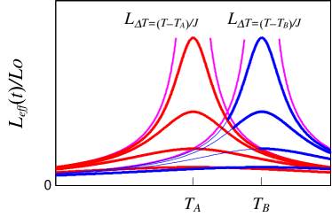
Figure 2: (Color online) A schematic illustration of the temperature profiles of the effective domain size around the working temperatures $T_{A}$ and $T_{B}$. The solid and dotted lines represent the effective domain size $L_{\rm eff}(t)$ at logarithmically separated times $t$ during isothermal aging at $T_{A}$ and $T_{B}$ respectively.

Let us now consider more generally what is happening on the reference states associated with different environments during isothermal aging, i.e. $R\neq A$ . As illustrated schematically in Fig. 2, the domains of the reference states at different environments $R\neq A$ will grow with time up to the overlap length between $\Gamma^{A}$ and $\Gamma^{R}$. Concerning this point it is useful to note the relation between the projections $\tilde{s}^{R}_{i}(t)$ and $\tilde{s}^{A}_{i}(t)$ given by,

$$\tilde{s}^{R}_{i}(t)=O^{AR}_{i}\tilde{s}^{A}_{i}(t),$$ (8)

which immediately follows from Eq. (6). Here $O_{i}^{AR}$ is the overlap between the equilibrium state $\Gamma_{A}$ and $\Gamma_{R}$ defined in Eq. (2). The spatial pattern of overlap $O_{i}^{AR}$ is roughly uniform over the length scale of the overlap length $L_{\Delta T}$ between $\Gamma_{A}$ and $\Gamma_{R}$. Beyond $L_{\Delta T}$, however, the configuration of the overlap $O_{i}^{AR}$ is random. Then it follows that the growth of domains belonging to $\Gamma_{A}$ ( and $\bar{\Gamma}_{A}$) only contributes to the growth of domains belonging to $\Gamma_{R}$ (and $\bar{\Gamma}_{R}$) up to the overlap length. Thus we expect that at environment $R$ the typical domain size, which we denote as effective domain size $L_{\rm eff}(t)$, should scale as,jonyosnor2002 ; jonyosnor2003

$$L_{\rm eff}(t)=L_{\Delta T}F\left(\frac{L_{T_{A}}(t)}{L_{\Delta T}}\right).$$ (9)

The scaling function $F(x)$ reflects the following three regimes as the age of the system, $t_{\rm w}$, increases:

1. Accumulative regime

   At length scales much shorter than the overlap length $L_{\Delta T}$, the growth of the domains belonging to $\Gamma_{A}$ leads to the growth of the domains belonging to $\Gamma_{R}$ such that $L_{\rm eff}(t_{\rm w})=L_{T_{A}}(t_{\rm w})$. This yields

   $$\lim_{x\to 0}F(x)=x.$$ (10)

2. Weakly perturbed regime

   As we discussed in the previous subsection, the chaos effect emerges gradually at length scales shorter than the overlap length. We now want to determine the first correction term to Eq. (10) due to defects at the scale of $L_{T_{A}}(t)$. Intuitively we assume that $L_{\rm eff}$ is analytic and an even function of $\Delta T$ (and $\Delta J$). We also expect that the correction term is an analytic function of $p_{\rm minor}$ [See Eq. (5)] which is proportional to $|\Delta T|$ (and $|\Delta J|$). Combining these we find that the fist correction term should be $O(p^{2}_{\rm minor})$ leading tofoot-correction-term

   $$F(x)=x(1-cx^{2\zeta})\qquad x\ll 1.$$ (11)

   We note that because of defects at length scales $L\ll L_{T_{A}}(t)$ the order parameter $\rho_{R}$ [Eq. (7)] is smaller than $\rho_{A}=1$.

3. Strongly perturbed regime

   The domains belonging to $\Gamma_{R}$ can by aging at $A$ only grow to the size of the upper bound $L_{\Delta T}$, yielding $L_{\rm eff}(t_{\rm w})=L_{\Delta T}$. This requires

   $$F(x)=1\qquad x\gg 1.$$ (12)

II.4 Relaxation after shift of working environments

Let us now consider a shift of working environment $A\to B$, after aging the system in the environment $A$ for a time $t_{\rm w}$. $\Gamma_{B}$ is the reference state since the working environment is now $B$. Just after the $T$-shift, the sizes of the domains $\Gamma_{B}$ associated with the environment $B$ (at temperature $T_{B}$) is given by the effective domain size $L_{\rm eff}(t_{\rm w})$ in Eq. (9) (see Fig. 2). Thus the spin configuration just after the temperature shift $T_{A}\to T_{B}$ is equivalent to that after usual isothermal aging done at $B$ for a certain waiting time $t_{\rm eff}$ (after direct temperature quench from above $T_{\rm g}$ down to $T_{B}$). The effective time, $t_{\rm eff}$, is defined through

$$L_{T_{B}}(t_{\rm eff})=L_{\rm eff}(t_{\rm w}).$$ (13)

Since $L_{\rm eff}(t_{\rm w})$ is limited by the overlap length $L_{\Delta T}$ rejuvenation occurs after the temperature (or bond)- shifts: the system looks younger [i.e. $L_{T_{B}}(t_{\rm eff})<L_{T_{A}}(t_{\rm w})$] than it would have been if the aging was fully accumulative [i.e. $L_{T_{B}}(t_{\rm eff})=L_{T_{A}}(t_{\rm w})$].

The effective time $t_{\rm eff}$ can be determined experimentally by measuring the ZFC relaxation after temperature and bond shifts (see Sec. IV). As in the isothermal case, lunetal83 a crossover occurs between quasi-equilibrium and out-of-equilibrium dynamics at $L_{T_{B}}(t)\sim L_{T_{B}}(t_{\rm eff})$, where $L_{T_{B}}(t)$ is the length scale on which the system is observed at time $t$ after the temperature (or bond) shift.

Now let us turn our attention to what happens to the amplitude of order parameters within the domains after $T$-shifts,

• The order parameter $\rho_{B}$ within domains belonging to $\Gamma_{B}$ evolves as follows. Although the system is essentially equilibrated with respect to $B$ up to the effective domain size $L_{\rm eff}(t_{\rm w})$, it contains some defects which cause a certain reduction of the order parameter. These defects are progressively eliminated after the $T$-shift and $\rho_{B}$ approaches the full amplitude $1$. At time $t$ after the shift of environment, such defects smaller than $L_{T_{B}}(t)$ are eliminated, but the larger ones still remain. Thus, this process finishes once defects as large as the domain size $L_{\rm eff}$ are removed. The time scale needed to finish this transient process is given by

  $$L_{T_{B}}(t_{\rm trans})=L_{\rm eff}$$ (14)

  thus $t_{\rm trans}\sim t_{\rm eff}$ because of Eq. (13).

• The order parameter within domains belonging to equilibrium states at other temperatures $T\neq T_{B}$ evolves as follows. At length scales greater than $L_{\Delta T=(T-T_{B})/T}$ (see Fig. 2) the domains grown before the $T$-shift suffer a progressive reduction of the order parameter. However, the spatial pattern of the sign of the bias remains the same as before the $T$-shift (see Fig. 3). This is a very important point that we discuss in detail in sec. II.5.

Let us also remark that the population of thermally active droplets at a certain scale $L$, which is proportional to fishus88eq $(k_{\rm B}T/J)(L/L_{0})^{-\theta}$, cannot follow sudden changes of the working temperatures, but needs a certain time to be switched off (or switched on). Progressive adjustments of the population of thermally active droplets take place on the time scale $t_{\rm trans}$ defined in Eq. 14.

In experiments, the progressive elimination of the remanent defects on domains belonging to $\Gamma_{B}$ after the shifts should give rise to certain excessive contributions to the relaxation of the magnetic susceptibility with the duration time $t_{\rm trans}$ given above. The amplitude of the excessive response is expected to be proportional to $\Delta T$ or $\Delta J$. This is because both the population of the isolated defects due to the chaos effect in the weakly perturbed regime (see Eq. (5)) and the excessive thermal droplets are proportional to $\Delta T$ or $\Delta J$.

II.5 Relaxation under cyclings of working environments

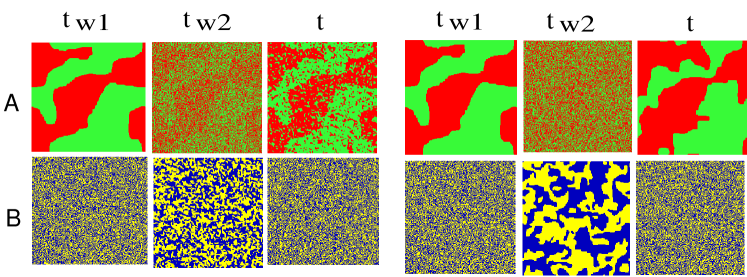
Figure 3: (Color online) An illustration of the evolution of ghost domains in a “perturbation-healing” protocol at large length scales. The above pictures are generated by an artificial simulation: Monte Carlo simulation is performed on a set of Ising spins on a square lattice by cycling the working Hamiltonian given by Mattis models whose ground states are exactly given by $\sigma^{A}$ and $\sigma^{B}$ (see the notefootmattis for the details). The different colors represent the sign $+$ and $-$ of the projections $\tilde{s}^{A}_{i}(t)$ (top figures) and $\tilde{s}^{B}_{i}(t)$ (bottom figures) at the end of initial aging state of duration $t_{\rm w}$ , at the end of the perturbation stage of duration $\tau_{\rm p}$ and after time $\tau_{\rm h}$ in the healing stage. Here the backbone spin configuration of the target equilibrium states $\sigma^{A}$ and $\sigma^{B}$ are completely unrelated random configurations so that the local overlap $O^{AB}_{i}=\tilde{s}^{A}_{i}(t)\tilde{s}^{B}_{i}(t)=\sigma^{A}\sigma^{B}$ (see Eq. (8)) is a completely random configuration: the overlap length is just $1$ in the unit lattice. The remanent bias at the end of the perturbation stage is found as (left) $\rho_{\rm rem}\sim 0.15$ and (right) $\rho_{\rm rem}\sim 0.04$. In the former the human eyes just barely distinguish the ghost domains, whereas in the latter the domains have become indistinguishable. In both cases, the strength of the bias increases up to $O(1)$ in the healing stage: (left) $\rho_{\rm rec}\sim 0.59$ and (right) $\rho_{\rm rec}\sim 0.58$.

We are now in position to discuss dynamics under cycling of working environments such as temperature cycling. Here we consider the simplest protocol. 1) Initial aging stage - after a temperature quench from above $T_{\rm g}$, the system is aged for a time $t_{\rm w_{1}}$ within environment $A$ - ($T_{A},{\cal J}_{A}$). 2) Perturbation stage - Then a “perturbation” is applied and the system is aged a time $t_{\rm w_{2}}$ at the new environment $B$ - ($T_{B},{\cal J}_{B}$). 3) Healing stage - finally the working environment is brought back to $A$ where the spin structure obtained in the initial aging stage slowly “heals” from the effects of the perturbation.

II.5.1 Weakly perturbed regime

Let us focus on what is happening on length scales shorter than the overlap length $L_{\Delta T}$ during the one-step cycling introduced above. This will be relevant for observations at correspondingly short time scales in experiments and simulations. The effect of the change of working environments should be perturbative in the weakly perturbed regime $L<L_{\Delta T}$ as we discuss below.

During the perturbation stage, the growth of domains belonging to $\Gamma_{B}$ introduces rare defects of size $L$ on top of the domains belonging to $\Gamma_{A}$ with a probability proportional to $(L/L_{\Delta T})^{\zeta}\ll 1$ (see Eq. (5)). Since the probability is low, these defects are isolated from each other. During the healing stage, these island like objects are progressively removed one by one from the small ones up to larger ones. Since the maximum size of such a defect is $L_{B}(t_{\rm w_{2}})$, we find that the removal of the defects will be completed in a time scale $t_{\rm rec}^{\rm weak}$ given by

$$L_{A}(t_{\rm rec}^{\rm weak})=L_{B}(t_{\rm w_{2}}).$$ (15)

Here the super-script “weak” indicates that the formula is valid only in the weakly perturbed regime. After this recovery time the original state of interior of the domains belonging to $\Gamma_{B}$ is restored. Finally let us also note that domain size at A continues to grow during the aging at B and vice-versa within the weakly perturbed regime.

II.5.2 Strongly perturbed regime

Suppose that the length scales explored during the three stages $L_{T_{A}}(t_{\rm w_{1}})$, $L_{T_{B}}(t_{\rm w_{2}})$ and $L_{T_{A}}(t)$ are all greater than the overlap lengths $L_{\Delta T}$. Then, the strongly perturbed regime of the chaos effect (see Sec. II.2) which appears at length scales greater than the overlap length $L_{\Delta T}$ should come into play. Figure 3 gives an illustration of how projections $\tilde{s}_{i}^{A}(t)$ and $\tilde{s}_{i}^{B}(t)$ evolves at length scales greater than the overlap length. The unit of length scale is chosen to be the overlap length $L_{\Delta T}$. Thus the pattern of the local overlaps $O^{AB}_{i}$ is completely random beyond the unit length scale.

In the initial aging stage, the domains belonging to $\Gamma^{A}$ grow up to the size $L_{T_{A}}(t_{\rm w_{1}})$. The amplitude of the order parameter within the domains has the full amplitude ($1$) everywhere.

In the perturbation stage, the system is relaxing in the environment $B$. Since the spin configuration before the perturbation stage is completely random with respect to $B$ beyond the overlap length $L_{\Delta T}$, the domains belonging to $\Gamma^{B}$ grow independently of the previous aging. In the meantime, the domains belonging to $\Gamma^{A}$ become “ghost” like, i.e. they keep their overall “shape” while their interior becomes noisy due to the growth of domains belonging to the reference state $B$. The remanent strength of the order parameter of $A$ defined in Eq. (7)

$$\rho_{\rm rem}(t)=\left|\frac{1}{{\cal N}_{A}}\sum_{i\in\mbox{ a domain of }\Gamma_{A}}\tilde{s}^{A}_{i}(t)\right|$$ (16)

slowly decays with time $t$. Here ${\cal N}_{A}\sim(L_{T_{A}}(t_{\rm w})/L_{0})^{d}$ is the number of spins belonging to a domain of $\Gamma_{A}$. After time $t$ from the beginning of the perturbation stage it becomes, yoslembou2001 ; yos2003

$$\rho_{\rm rem}(t)\sim\left(\frac{L_{T_{B}}(t)}{L_{\Delta T}}\right)^{-\bar{\lambda}}$$ (17)

where $\bar{\lambda}$ is a dynamical exponent. The crucially important point is that the spatial pattern of the sign of the local bias (order parameter) - with decreasing amplitude of strength $\rho_{\rm rem}(t)$ - is preserved during the perturbation stages. We call this spatial structure a ghost domain. Such ghost domains are responsible for the memory effect allowed after full rejuvenation induced by the chaos effect.

In the healing stage, the domains belonging to $\Gamma_{A}$ start to grow from the unit length scale $L_{\Delta T}$ all over again. However, the initial condition for this healing stage is not completely random, since ghost domains with bias $\rho_{\rm rem}(t_{\rm w_{2}})$ exist. We thus need to consider domain growth with slightly biased initial condition.BK92 The bias now increases with time as,yos2003

$$\rho_{\rm rec}(t;\rho_{\rm rem})\sim\rho_{\rm rem}(t_{\rm w_{2}})\left(\frac{L_{T_{A}}(t)}{L_{\Delta T}}\right)^{\lambda}.$$ (18)

Since the size of the ghost domain itself is finite, it also continues to grow during the healing stage. Following Ref. yoslembou2001, we call the growth of the bias inside a ghost domain during the healing stage inner-coarsening and the further growth of the size of the ghost domain itself outer-coarsening.

The growth of the bias stops when the bias (order parameter) saturates to the full amplitude. This defines the recovery time $t_{\rm rec}^{\rm strong}$,

$$\rho_{\rm rec}(t_{\rm rec}^{\rm strong};\rho_{\rm rem})\sim 1\qquad L(t_{\rm rec}^{\rm strong})/L_{\Delta T}\sim\rho_{\rm rem}^{-1/\lambda}.$$ (19)

Combining this with Eq. (17) the relation yos2003

$$\frac{L_{T_{A}}(t_{\rm rec}^{\rm strong})}{L_{\Delta T}}=\left(\frac{L_{T_{B}}(t_{\rm w_{2}})}{L_{\Delta T}}\right)^{\bar{\lambda}/\lambda}$$ (20)

is obtained. Here, the super-script “strong” indicates that the formula is valid only in the strongly perturbed regime.

An important remark is that the two exponents $\lambda$ and $\bar{\lambda}$ are in general different. In Ref. BK92, , a scaling relation $\bar{\lambda}+\lambda=d$ was found. Only in the special case $\lambda=\bar{\lambda}$, which happens e.g. in the spherical model considered in Ref. yoslembou2001, , the relation Eq. (20) is accidentally simplified to $L_{T_{A}}(\tau^{\rm strong}_{rec})=L_{T_{B}}(\tau_{\rm p})$. Concerning the exponent $\bar{\lambda}$ the inequality is proposed as, fishus88noneq $d/2\leq\bar{\lambda}<d.$ Combining that with $\bar{\lambda}+\lambda=d$, a useful inequality is obtained, yos2003

$$\bar{\lambda}/\lambda\geq 1.$$ (21)

In Ref. yos2003, , the 4d Ising EA model was studied and it was found that $\bar{\lambda}\sim 3.2$ and $\lambda\sim 0.8$. In this case and also in general for 3d systems the recovery time is very large $t_{\rm rec}^{\rm strong}\gg t_{\rm rec}^{weak}$.

The above results are markedly different from what one would expect from conventional “real space” or “phase space” arguments which neglect the role of bias. If such a mechanism causing a symmetry breaking is absent, the “new domains” grown during the healing could often have the wrong sign of bias with respect to the original one leading to total erasure of memory. In contrast to the hierarchical phase space models, vinetal96 the ghost domain scenario predicts memory also in the positive $T$-cycling ($T_{A}<T_{B}$) case. Indeed such examples are already reported (see Fig 6. in Ref. vinetal96, and Fig. 3 in Ref.  Gbergetal90, ).

II.5.3 Multiplicative rejuvenation effect

The above considerations for the one step cycling can be extended to multi-step cycling cases. At large length/time scales beyond the overlap length, some quite counter-intuitive predictions follow due to the multiplicative nature of the noise effect.yoslembou2001 For example, in a $T$-cycling $T_{A}(t_{\rm w_{1}})\to T_{B}(t_{\rm w_{2}})\to T_{C}(t_{\rm w_{3}})\to T_{A}$, the amplitude of the order parameter of $A$ is reduced to $\rho_{\rm rem}\sim\rho_{B}\times\rho_{C}$ in the end of the 2nd perturbation. Here $\rho_{B}$ and $\rho_{C}$ represent reductions due to domain growth at $B$ and $C$. Thus, the recovery time $t_{\rm rec}^{\rm strong}$ of the order parameter of $A$ becomes,

$$\frac{L_{T_{A}}(t_{\rm rec}^{\rm strong})}{L_{\Delta T}}=\left(\frac{L_{T_{B}}(t_{\rm w_{2}})}{L_{\Delta T}}\frac{L_{T_{C}}(t_{\rm w_{3}})}{L_{\Delta T}}\right)^{\bar{\lambda}/\lambda}.$$ (22)

This tells that sequential short time perturbations can cause huge recovery times. Let us note that this multiplicative rejuvenation effect is absent at length/time scales smaller than the overlap length $L_{\Delta T}$. At such short length scales, changes of temperature (or bonds) only amount to put isolated island like defects on the domains which rarely overlap with each other. The multiplicative effect discussed above is hardly expected within conventional pictures which do not contain the time evolution of the bias (order parameter).

II.6 Freezing of aging by slow changes of working environments - heating/cooling rate effects

The effect of finite heating/cooling rate is a very important problem from an experimental point of view. Even the fastest cooling/heating rates such as those used in “temperature quench” experiments are always extremely slow compared to the atomic spin flip time $\tau_{\rm m}\sim\hbar/J\sim 10^{-13}$ s. Typically the maximum experimental heating/cooling rate is $v_{T}\sim O(10^{-1})$ K/s and $T_{\rm g}\sim O(10)$ K (see Appendix  B), which in simulations would be equivalent to an extremely slow heating/cooling rate of $v_{T}\sim 10^{-15}T_{\rm g}/{\rm MCS}$. Thus, the instantaneous changes of the working environments assumed in the previous sections are very unrealistic, at least experimentally.

Nonetheless, we expect that the effect of a finite heating/cooling rate can be taken into account by introducing a characteristic length scale $L_{\rm min}(v_{T},T)$. As discussed in Ref. yos2003, , it is natural to expect that the competition between accumulative and chaotic (rejuvenation) processes during a slow change of working environments, either temperature or bond changes, results in a sort of freezing of aging, such that the effective domain size with respect to the temporal working environment becomes a constant in time $L_{\rm min}(v_{T},T)$. This domain size is expected to decrease when the rate of the changes increases, e.g. the heating or cooling rate $v_{T}$. The characteristic length $L_{\rm min}(v_{T},T)$ can be seen as a renormalized overlap length in the following senses:

• The frozen age $t_{\rm min}$ given by $L_{T}(t_{\rm min})=L_{\rm min}(v_{T},T)$ sets the minimum time scale for the start of the domain growth when the target temperature $T$ is just reached after continuous temperature changes. This effect can be readily seen experimentally as we discuss in Secs. IV.1 and B.2.

• The overlap length $L_{\Delta T}$ appearing in equations Eq. (20) and Eq. (22) should be replaced by $L_{\rm min}(v_{T},T)$. The latter should be greater than the overlap length $L_{\Delta T}$ between the equilibrium states at two temperatures connected by a continuous temperature change. Thus, the finiteness of the heating/cooling rate can significantly reduce the recovery times for the memories.

Indeed, it is known from previous experimental studies that cooling/heating rate effects are non-accumulative and that it is only the rate very close to the target temperature that affects the observed isothermal aging behavior.jonetal98 ; jonetal99 However, within this narrow temperature region around the target temperature, heating/cooling rate effects were found to be relevant, but as long as the employed observation time is made long even a cooling with $v_{T}\sim O(10^{-1})$ K/s can be regarded as a “quench” that allows experimental observations of non-equilibrium dynamical scaling properties of isothermal aging starting from a random spin configuration. vinetal96 ; jonetal2002PRL An interpretation of this feature would be that the observation times used in the experiments are actually larger than the effective age $t_{\rm min}$ related to the renormalized overlap length. This remarkable feature is quite different from that of other glassy systems governed by simple thermal slowing down, such as super-cooled liquids,lehnag98 in which the effect of aging at different temperatures during the heating/cooling only add up accumulatively. It may be argued that the unusual cooling rate independence of the dynamics in spin glasses already in itself supports the relevance of the temperature-chaos concept.

II.7 Comparisons to the classical Kovacs effect

The mechanisms and nature of the memory effects involving length scales shorter and longer than the overlap length are markedly different within the ghost domain scenario. After a change of working environments involving only short length scales the chaos effect is weak (perturbative) and the system is not rejuvenated. Such non-chaotic perturbative effects yield, as discussed in Sec. II.5.1, the trivial recovery time given by Eq. (15). This recovery time fits well with conventional intuition based on “length scales” or “phase space”. Such effects may be understood as classical memory effects in a fixed energy landscape known as Kovacs effects in polymer glasses,kovacs which do not accompany a real rejuvenation. It is reasonable to expect that Kovacs effects exist in a broad class of systems bouchaud2000 ; berbou2002 ; beretal ; bbdg2003 as far as the chaos effects are absent or irrelevant. The fixed energy landscape picture is valid only at length scales shorter than the overlap length where defects are approximately independent of each other. For perturbations involving length scales greater than $L_{\Delta T}$ this picture becomes totally invalid and the scenario outlined above for the strongly perturbed regime is required.

III Introduction to experiments and simulations

Experiments. — The non-equilibrium dynamics of two canonical spin glasses was investigated using superconducting quantum interference device (SQUID) magnetometry. The samples are a single crystal of Fe_0.5Mn_0.5TiO₃ ($T_{\rm g}\approx 21.3$ K), the standard Ising spin-glass,itoetal86 ; itoetal90 and a polycrystalline sample of the Heisenberg Ag(11 at% Mn) spin-glass ($T_{\rm g}\approx 32.8$ K). The experiments were performed in non-commercial SQUID magnetometers,magetal97 designed for low-field measurements and optimum temperature control (see Appendix B for details).

Experimental results for the two samples will be presented using the following thermal procedures:

1. In an isothermal aging experiment the sample is quenched (cooled as rapidly as possible) from a temperature above the transition temperature to the measurement temperature $T_{\rm m}$ in the spin glass phase. In dc measurements, the relaxation of the ZFC magnetization is recorded in a small probing field after aging the sample in zero field for a time $t_{\rm w}$ at the measurement temperature.

2. In a $T$-shift experiment (Sec. IV.1) the sample is, after a quench, first aged at $T_{\rm i}$ before measuring the relaxation at $T_{\rm m}=T_{\rm i}+\Delta T$.

3. In a $T$-cycling experiment (Sec. V.1) the sample is first aged at $T_{\rm m}$, then at $T_{\rm m}+\Delta T$ and subsequently the relaxation is recorded at $T_{\rm m}$.

4. In a temperature memory experimentjonetal98 ; matetal2001 (Sec. VI) the system is cooled from a temperature above the transition temperature to the lowest temperature. The cooling is interrupted at one or several temperatures in the spin glass phase. The magnetization is subsequently recorded on re-heating.

In experiments (i)–(iii) all temperature changes are made with the maximum cooling rate ($v_{\rm cool}\sim 0.05$ K/s) or maximum heating rate ($v_{\rm heat}\sim 0.5$ K/s). A temperature quench therefore refers to a cooling with the maximum cooling rate. The magnetic fields employed in the experiments are small enough ($h\approx 0.1-1$ Oe) to ensure a linear responsematetal2001 of the system.

Figure 4: (Color online) Ac susceptibility vs time after a temperature quench. A temperature cycling from 30 K to 28 K and back to 30 K is shown as pluses. The solid lines are the isothermal aging at 28 K and 30 K. After the negative $T$-shift from 30 K to 28 K the system is completely rejuvenated. Still, after the $T$-cycling it keeps a memory of the first aging at 30 K. $f=510$ mHz.

To shortly illustrate the rejuvenation and memory phenomena, that are examined in detail in this article, we show in Fig. 4 a negative $T$-cycling experiment on the Ag(11 at% Mn) sample. The ac-susceptibility is measured as function of time after a temperature quench. The system is aged at 30 K for 3000 s, afterward the temperature is changed to 28 K for 3000 s, and finally it is changed back to 30 K. The isothermal aging at 30 K and 28 K are shown as references. We first notice that the aging at 28 K is the same in the cycling experiment as after a direct quench. Hence, at 28 K, the system appears unaffected by the previous aging at 30 K—the system is completely rejuvenated at the lower temperature. However, some time ($t_{\rm rec}$) after changing the temperature back to 30 K the ac signal is the same as if the aging at 28 K had not taken place; despite the rejuvenation at 28 K the system keeps a memory of the aging at 30 K. One of our major interests is to clarify if the memory recovery process with duration $t_{\rm rec}$ can be understood in terms of the ghost domain picture (Sec. II).

Simulations. – Standard heat-bath Monte Carlo simulations of the EA Ising model (introduced in Sec. II.1) on the 4 dimensional hyper cubic lattice ($T_{\rm g}=2.0J$)bercam97 were performed following protocols (i)-(iii), but using a bond change ${\cal J}_{A}\to{\cal J}_{B}$ instead of a temperature change. The initial conditions are random spin configurations to mimic a direct temperature quench (with $v_{T}=\infty$) to $T<T_{\rm g}$. Detailed comparisons of the effects of bond perturbations and temperature changes allows us to clarify the common mechanism of rejuvenation and memory effects. An important advantage of the numerical approach is that the dynamical length scale $L_{T}(t)$ can be obtained directly in the simulations.rieger95 ; yoshuktak2002 Details of the model and the simulation methods are given in Appendix C.

IV Rejuvenation effects after temperature and bond shifts

In this section, we present a quantitative study of the rejuvenation effect using $T$-shift experiments and bond-shift simulations.

IV.1 Temperature-shift experiments

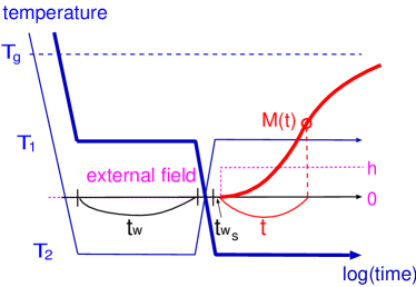
Figure 5: (Color online) Schematic representation of a twin $T$-shift experiment. In the experiment represented using the thick line, $(T_{\rm i},T_{\rm m})=(T_{1},T_{2})$, while $(T_{\rm i},T_{\rm m})=(T_{2},T_{1})$ in the experiment represented by the thin line. In ac experiments, $\chi(t)$ is also monitored during the halt at $T_{\rm i}$. In order to ensure thermal stability at $T_{\rm m}$, a short waiting time $t_{\rm ws}=3$ s is needed before applying the magnetic field and recording the ZFC relaxation.footstab

In a $T$-shift experiment, the system is quenched to the initial temperature $T_{\rm i}(<T_{\rm g})$, where it is aged a certain time $t_{\rm w}$; the temperature is changed to the measurement temperature $T_{\rm m}=T_{\rm i}+\Delta T$, and ZFC-relaxation $M(t)$ (or ac susceptibility relaxation) is recorded. Conjugate experiments with $T_{\rm i}$ and $T_{\rm m}$ being interchanged are called twin $T$-shift experiments (see Fig. 5).

The effective age ($t_{\rm eff}$) of the SG system at $T_{\rm m}$, due to the previous aging at $T_{\rm i}$, can be determined either from the maximum in the relaxation rate $S(t)=h^{-1}dM(t)/d\log t$ of ZFC relaxation measurements, graetal88 ; sanetal88 ; jonyosnor2002 or by the amount of time that an ac susceptibility relaxation curve measured after a $T$-shift, needs to be shifted to merge with the reference relaxation curve measured without a $T$-shift. mametal99 ; dupetal2001 ; takhuk2002 We will here show that both ways to derive $t_{\rm eff}$ are consistent, discuss the experimental limitations that determine the accuracy of the estimations and indicate in which time window the derived effective age gives non-trivial information. Finally, we will use the extracted $t_{\rm eff}$ data to quantitatively analyze the emergence of the chaos effect.

IV.1.1 ZFC relaxation after $T$-shifts

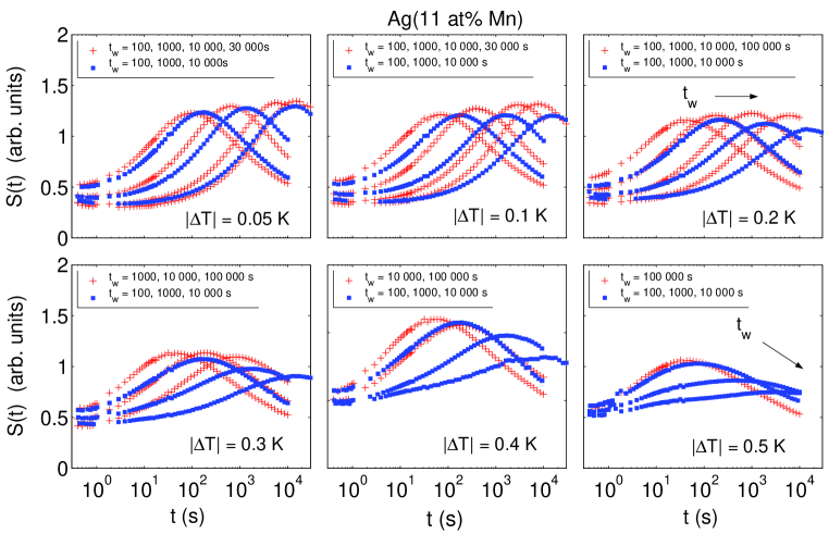
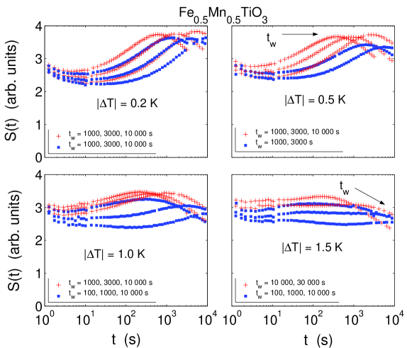
Figure 6: (Color online) Relaxation rate vs time after positive and negative twin $T$-shift measurements. Pluses are positive $T$-shifts $(T_{1},T_{2})$, while squares are negative $T$-shifts $(T_{2},T_{1})$. (a) Ag(11 at% Mn) : $T_{1}=30-|\Delta T|$ K and $T_{2}=30$ K. (b) Fe_0.5Mn_0.5TiO₃ : $T_{1}=19-|\Delta T|$ K and $T_{2}=19$ K. Note that for each $\Delta t$ the peak position $t_{\rm max}$ increases with $t_{\rm w}$ and the maximum in $S(t)$ broadens, which suggests that these data reflect the weakly perturbed regime of the temperature-chaos effect. (See later Fig. 11 for the corresponding data of bond-shifts in the 4d EA model.)

The relaxation rate after twin $T$-shift experiments are shown in Fig. 6 for the two samples. The effective age ($t_{\rm eff}$) of the system after a $T$-shift is determined from the time $t_{\rm peak}$ corresponding to the maximum in $S(t)$ (see Appendix B.2 for details). The shape of the $S(t)$ curves changes after both negative and positive $T$-shifts; the maximum in $S(t)$ becomes broader with increasing $|\Delta T|$ (and for a certain $|\Delta T|$ also with increasing $t_{\rm w}$). Due to this broadening $t_{\rm peak}$ becomes less well-defined and thus $t_{\rm eff}$ less accurate. A broadening of $S(t)$ with increasing $|\Delta T|$ is observed for both samples, but it should be noted that the temperature shifts employed for the Fe_0.5Mn_0.5TiO₃ sample are much larger than those for the Ag(11 at% Mn) sample. That the data in Fig. 6 shows an increase of $t_{\rm peak}$ with $t_{\rm w}$ indicates that the $\Delta T$’s are small enough to belong to the weakly perturbed regime, i.e. $L_{T_{i}}(t_{\rm w})\lesssim L_{\Delta T}$. The broadening of the relaxation rate can hence be explained by the weak chaos effect (see Sec. II.3); during the aging at $T_{\rm i}$ ghost domains grow at nearby temperatures up to the overlap length. The interior of these ghost domains contain defects or noise and do therefore not have full amplitude of the order parameter [Eq. 7]. These defects are progressively eliminated after the $T$-shift giving rise to extra responses (see Sec. II.4). Such extra responses are reflected in the ZFC magnetization measurements as a broadening of $S(t)$.

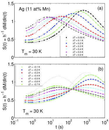
Figure 7: (Color online) Relaxation rate vs time after aging the Ag(11 at% Mn) sample at (a) $T_{\rm i}=29.95$, 29.9, 29.8, 29.7, 29.6, 29.5, 29.4 K (b) $T_{\rm i}=30.1$, 30.2, 30.3, 30.4, 30.5, 30.6, 30.7 K using $t_{\rm w}$ = 1000 s and $T_{\rm m}$ = 30 K. Dotted lines are ordinary isothermal aging curves with $t_{\rm w}$ = 3 and 1000 s. (See Fig. 3 in Ref. djujonnor99, for the case of a Cu(Mn) spin glass.)

For the Ag(11 at% Mn) sample, if $|\Delta T|$ is increased even further the maximum in $S(t)$ again becomes narrower, as can be seen in Fig. 7, where positive and negative $T$-shift with $T_{\rm m}=30$ K and $t_{\rm w}=1000$ s are shown for various values of $T_{\rm i}$. For larger enough $|\Delta T|$ the peak position $t_{\rm peak}$ piles up around $t_{\rm min}$. This $t_{\rm min}$ ($L_{\rm min}=L_{T}(t_{\rm min})$) is the shortest effective age (domain size) in the system after a $T$-change and it depends on the cooling/heating rate as discussed in Sec. II.6 and Appendix B.2. A similar behavior has been observed in a Cu(Mn) spin glass, as shown in Fig. 3 of Ref. djujonnor99, . That $t_{\rm peak}$ saturates to $t_{\rm min}$ indicates that $L_{\Delta T}<L_{\rm min}$; the experimentally accessible times $t_{\rm w}$ [or lengths $L_{T_{i}}(t_{\rm w})$] lie in the strongly perturbed regime. However since the overlap length is “hidden” behind the domains grown during the $T$-change, these measurements do not give any direct information about the overlap length.

For the Fe_0.5Mn_0.5TiO₃ sample the strongly chaotic regime could not be observed within the temperature range used in the experiments reported in the present section. However, we expect to see a narrowing of $S(t)$ also for the Fe_0.5Mn_0.5TiO₃ sample if $|\Delta T|$ is made large enough.

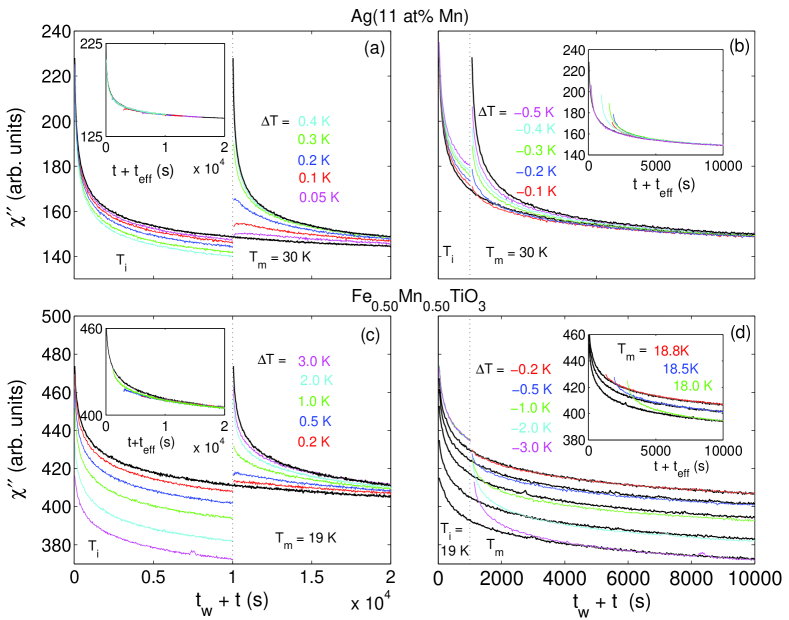
Figure 8: (Color online) $\chi^{\prime\prime}$ vs time measured for positive and negative $T$-shift experiments. (a) The Ag(11 at% Mn) sample is aged at $T_{i}=29.95$, 29.9, 29.8, 29.7, 29.6 K for $t_{\rm w}=10\,000$ s before changing the temperature to $T_{m}=30$ K. (b) It is aged at $T_{i}=30.1$, 30.2, 30.3, 30.4, 30.5 K for $t_{\rm w}=1000$ s before changing the temperature to $T_{m}=30$ K. (c) The Fe_0.5Mn_0.5TiO₃ sample is aged at $T_{\rm i}=18.8$, 18.5, 18.0, 17.0, 16.0 K for $t_{w}=10\,000$ s before changing the temperature to $T_{m}=19$ K. (d) It is aged at $T_{\rm i}=19$ K for $t_{w}=1000$ s before changing the temperature to $T_{\rm m}=18.8$, 18.5, 18.0, 17.0, 16.0 K. The thick lines are the (reference) isothermal aging curves starting from $t_{\rm w}+t=0$ and $t_{\rm w}+t=t_{\rm w}$. The insets show $\chi^{\prime\prime}(T_{\rm m})$ vs $t+t_{\rm eff}$ with $t_{\rm eff}$ determined from ZFC relaxation experiments. $f=510$ mHz.

IV.1.2 ac susceptibility relaxation after $T$-shifts

In an isothermal aging experiment $\chi^{\prime\prime}(t)$ is recorded vs. time immediately after the quench (only allowing some time for thermal stabilization and stabilization of the ac signal). In a $T$-shift experiment, $\chi^{\prime\prime}(t)$ is continuously measured after the initial temperature quench to $T_{\rm i}$. In the following we choose $t=0$ immediately after the $T$-shift to $T_{\rm m}$.

$T$-shift ac relaxation measurements with $T_{\rm i}<T_{\rm m}$ (positive T-shift) are shown in Fig. 8(a,c). For large enough $\Delta T$ the relaxation curves after the $T$-shifts become identical to the reference isothermal aging curve. The $\Delta T/T_{\rm g}$ needed to make the aging at the lower temperature negligible is however much larger for the Fe_0.5Mn_0.5TiO₃ sample than for the Ag(11 at% Mn) sample. If the time scale of these $\chi^{\prime\prime}(t)$ curves are shifted by the effective time determined from the corresponding ZFC relaxation experiments reported before, they merge with the reference isothermal $\chi^{\prime\prime}(t)$ curve. This is true for both samples [see the insets of Fig. 8(a,c)], however a transient part of the curves at short times lies below the isothermal aging curve.

$T$-shift ac susceptibility relaxation measurements with $T_{i}>T_{m}$ (negative T-shift) are shown in Fig. 8(b,d). For the Ag(11 at% Mn) sample, the $T$-shift relaxation curves lie below the reference isothermal aging curve for small $|\Delta T|$. However for larger $|\Delta T|$ the $T$-shifted relaxation curves lie above the reference curve and for large enough $|\Delta T|$ the relaxation curves are identical to the isothermal aging curve (complete rejuvenation). For the Fe_0.5Mn_0.5TiO₃ sample, no complete rejuvenation can be observed even for $\Delta T=-3$ K ($\Delta T/T_{g}=-0.14$), whereas for the Ag(11 at% Mn) sample complete rejuvenation is already observed for $|\Delta T|/T_{g}\gtrsim 0.03$ on the examined time scales. Shifting the time scale by $t_{\rm eff}$, determined from ZFC relaxation experiments, makes the $T$-shift curve merge with the reference curve at long time scales as shown in the insets of the figures. At short time scales, a long transient relaxation exists during which $\chi^{\prime\prime}(t)$ lies above the reference curve.

The transient part of the susceptibility $\Delta\chi^{\prime\prime}$ shows nonmonotonic behavior with increasing $\Delta T$ in the case of negative T-shifts; $\Delta\chi^{\prime\prime}$ initially becomes larger but it eventually disappears for large $\Delta T$’s as $t_{\rm eff}\to 0$. These two features can be observed for the Ag(11 at% Mn) sample in Fig. 8(b) and complete rejuvenation ($t_{\rm eff}=0$ and $\Delta\chi^{\prime\prime}=0$) is shown in Fig. 4. However, only the initial increase of $\Delta\chi^{\prime\prime}$ can be observed for the Fe_0.5Mn_0.5TiO₃ sample in Fig. 8(d). The nonmonotonic behavior of $\Delta\chi^{\prime\prime}$ is consistent with the picture presented in Sec. II.4; in the weakly perturbed regime, the excess transient responses should be proportional to $\Delta T$ and the duration of the transient response $t_{\rm trans}$ is roughly the same as the effective time $t_{\rm eff}$, while in the strongly perturbed regime $\Delta\chi^{\prime\prime}\to 0$ as $t_{\rm eff}\to 0$, which is the limit of complete rejuvenation.

IV.1.3 Non-accumulative aging

The previous sections described how to determine the effective age ($t_{\rm eff}$) of the SG systems after a $T$-shift. The extracted effective age can now be used to examine if the aging is fully accumulative or not. The advantage of the twin $T$-shift method jonyosnor2002 is that it allows one to distinguish between the two cases although the growth law $L_{T}(t)$ is unknown. By plotting $t_{2}$ ($t_{\rm w}$ or $t_{\rm eff}$ at $T_{2}$) vs $t_{1}$ ($t_{\rm w}$ or $t_{\rm eff}$ at $T_{1}$), the sets of data from the positive $T$-shifts and the corresponding negative $T$-shifts should fall on the same line corresponding to $t_{2}=L_{T_{2}}^{-1}[L_{T_{1}}(t_{1})]$ if the aging is fully accumulative, while any deviation suggests emergence of rejuvenation (non-accumulative aging).

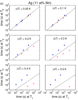
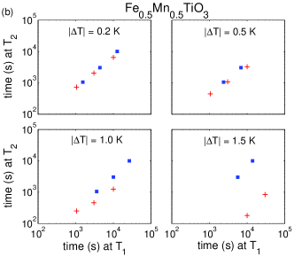
Figure 9: (Color online) Relation between $t_{\rm w}$ and $t_{\rm eff}$ in twin experiments - ($T_{1}$,$T_{2}$) shown as pluses and ($T_{2}$,$T_{1}$) shown as squares. (a) For the Ag(11 at% Mn) sample, $T_{1}=(30-|\Delta T|)$ K and $T_{2}=30$ K with $|\Delta T|=0.05$, 0.1, 0.2, 0.3, 0.4, 0.5 K ($0.015T_{\rm g}$). The solid line indicates fully accumulative aging $L_{T_{1}}(t_{1})=L_{T_{2}}(t_{2})$, calculated assuming logarithmic domain growth [Eq. 28]. (b) for the Fe_0.5Mn_0.5TiO₃ sample, $T_{1}=(19-|\Delta T|)$ K and $T_{2}=19$ K with $|\Delta T|=0.2$, 0.5, 1.0, 1.5 K ($0.064T_{\rm g}$).

Plots of $t_{1}$ vs $t_{2}$ are shown in Fig. 9. $t_{\rm eff}$ is determined from the twin $T$-shift ZFC relaxation experiments shown in Fig. 6. For the Ag(11 at% Mn) sample, the line of accumulative aging is shown in addition; a logarithmic domain growth law [Eq. (28)] has been used with parameters taken from previous studies.jonetal2002PRL ; jonyosnor2002 It can be seen for both samples that the aging is accumulative for small values of $|\Delta T|$ while for larger $|\Delta T|$ non-accumulative aging is observed (the data for positive and negative $T$-shifts do not any longer fall on the same line). There is however a large difference between the two samples as to how large values of $|\Delta T|/T_{\rm g}$ are required to introduce non-accumulative aging. A similar analysis of $t_{\rm eff}$ after twin $T$-shift experiments was recently performed on the 3d EA Ising model.takhuk2002 Only very weak rejuvenation effects could be observed for the Ising model on the time/length scales accessible by the numerical simulations even for such large $\Delta T/T_{\rm g}$ as 0.3.

IV.1.4 Evidence for temperature-chaos

Is the non-accumulative aging consistent with temperature chaos as predicted by the droplet model? In order to answer that question we need to transform timescales into length scales. In other words we need to know the functional form of the domain growth law. In Ref. jonetal2002PRL, it was shown that the ac relaxation data measured at different frequencies and temperatures are consistent with a logarithmic domain growth law [Eq. (28)]. The temperatures used in that study include those in Fig. 6 for the Ag(11 at% Mn) sample, but not for the Fe_0.5Mn_0.5TiO₃ sample. We therefore restrict the search of temperature-chaos to the Ag(11 at% Mn) sample.

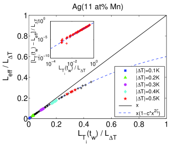
Figure 10: (Color online) Scaling plot of $L_{\rm eff}$ with $L_{\Delta T}=L_{0}(a|\Delta T|/T_{\rm g})^{-1/\zeta}$ with $a=6$ and $1/\zeta=2.6$. The fit is due to the scaling ansatz for the weakly perturbed regime [Eq. (11)] with c=0.4. The deviation from accumulative aging is shown in the inset and the line is the fit to the scaling ansatz for the weakly perturbed regime. (See Fig. 12 for the corresponding scaling plot of the data of bond-shifts in the 4 dim EA model.)

For the Ag(11 at% Mn) sample, we showed in Ref. jonyosnor2002, that positive and negative twin $T$-shifts can be made equivalent by plotting $L_{T_{\rm m}}(t_{\rm eff})$ vs $L_{T_{\rm i}}(t_{\rm w})$. This supports the expectation of the droplet theory bramoo87 ; fishus88eq that there is a unique overlap length between a given pair of temperatures. By scaling $L_{T_{\rm m}}(t_{\rm eff})$ and $L_{T_{\rm i}}(t_{\rm w})$ with the overlap length $L_{\Delta T}=L_{0}(a|\Delta T|/T_{\rm g})^{-1/\zeta}$, all data corresponding to different $T_{\rm i}$, $T_{\rm m}$, and $t_{\rm w}$ merge on a master curve if $1/\zeta=2.6$ (see Fig. 10). This master curve is consistent with the scaling ansatz in the weakly perturbed regime [Eq. (9-11)] as shown in the figure.

In the limit of strong chaos it is theoretically expected that $L_{T_{\rm m}}(t_{\rm eff})=L_{\Delta T}$ [Eq. (9) and (12)], and hence that the effective age of the system should only be given by the overlap length $L_{\Delta T}$ and not by the wait time $t_{\rm w}$. Our study is however strongly limited by the experimental time window. The upper limit $10^{4}-10^{5}$ s is set by how long we can wait for our experiments to finish, while the lower limit $t_{\rm min}$ is set by the cooling/heating rate and the time needed to stabilize the temperature (see Appendix B.2). For large $\Delta T\gtrsim 0.7$, $t_{\rm peak}$ is saturated to $t_{\rm min}$ (corresponding to $L_{\rm min}$) and obviously such values of $t_{\rm peak}$ cannot be used in the scaling plot in Fig. 10. $L_{\Delta T}$ cannot be observed directly in this regime, but the fact that $L_{\Delta T}<L_{\rm min}$ in itself give evidence for strong chaos within the experimental time (length) window.

Finally, we will make some comments on the validity of the scaling presented in Fig. 10. The quality of the scaling does not change significantly when altering the values of the parameters ($\tau_{m}=10^{-13}$ s, $T_{\rm g}=32.8$ K, $z\nu=7.2$, $\psi=1.2$, $J=T_{\rm g}$, and $\nu=1.1$ from Ref. jonyosnor2002, ), with one exception—symmetry between positive and negative $T$-shifts is obtained only if $\psi\nu\approx 1.3$. The x- and y-scale are completely arbitrary. We have intentionally chosen the constant $a$ so that the data appear to be rather close to the strong chaos regime.

IV.2 Bond shift simulations

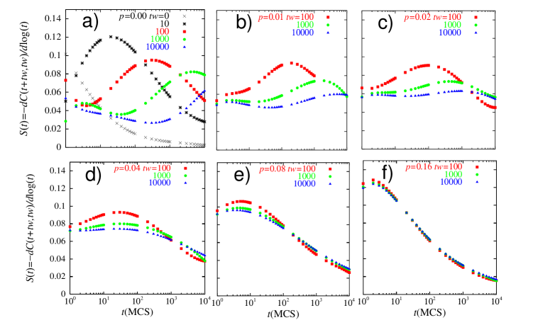
Figure 11: (Color online) The relaxation rate $S(t)=-dC(t+t_{\rm w},t_{\rm w})/\log(t)$ of the 4DEA model after different waiting times $t_{\rm w}$ with bond shifts of various strength $p$ at temperature $T=0.6T_{g}$.

We now present results of bond-shift simulations on the $\pm J$ EA model introduced in section II.1. Two sets of bonds ${\cal J}_{A}$ and ${\cal J}_{B}$ are prepared as explained in section II.2. Namely the set of bonds ${\cal J}_{B}$ is created from the set ${\cal J}_{A}$ by changing the sign of a small fraction $p$ of the bonds randomly. The protocol of the simulation is the following: a system with a certain set of bonds ${\cal J}^{A}$ is aged for a time $t_{\rm w}$, after which the bonds are replaced by ${\cal J}^{B}$ and the relaxation of the spin auto-correlation function

$$C_{\rm ZFC}(t+t_{\rm w},t_{\rm w})=(1/N)\sum_{i}\langle S_{i}(t_{\rm w})S_{i}(t+t_{\rm w})\rangle\,,$$ (23)

where $i$ runs over the $N$ Ising spins $S_{i}$ in the system, is recorded. The bracket $\langle\ldots\rangle$ denotes the averages over different realizations of initial conditions, thermal noises and random bonds. The subscript “ZFC” is meant to emphasize that this auto correlation function is conjugate to the ZFC susceptibility: if the fluctuation dissipation theorem (FDT) holds $(1-C_{\rm ZFC}(t))(J/T)$ becomes identical to the ZFC susceptibility. The relaxation rate $S(t)$ is extracted by computing the logarithmic derivatives numerically,

$$S(t)=-dC_{\rm ZFC}(t+t_{\rm w},t_{\rm w})/\log(t).$$ (24)

Usually the ZFC susceptibility is used to obtain the relaxation rate. Here, we used the auto-correlation function since it has much less statistical fluctuations. We note that FDT is well satisfied within what is called the quasi-equilibrium regime yoshuktak2002 so that $S(t)$ defined above yields almost the same effective time $t_{\rm eff}$ as obtained from the ZFC susceptibility. We remark that the autocorrelation function can be measured experimentally by noise-measurement technique HO02 .

In Fig. 11, we show some data of relaxation rates obtained at $T/J=1.2$ ($T/T_{g}=0.6$) for bond-shift simulations with wait times $t_{\rm w}=10^{2},10^{3},10^{4}$ and various strength of the perturbations $\Delta J/J\sim\sqrt{p}$ with $p$ in the range 0–0.16. For relatively small $p$ $(\lesssim 0.05)$, it can be seen that the peaks in the relaxation rate $S(t)$ become broader either by increasing $p$ or $t_{\rm w}$. Simultaneously, with increasing $p$, they become somewhat suppressed and their positions are slightly shifted to shorter times compared to the peaks of the reference curves for $p=0.0$ [Fig. 11(a)]. At larger $p$ $(\gtrsim 0.05)$, different features can be noticed. The relaxation rate $S(t)$ still becomes broader by increasing $t_{\rm w}$ but tends to saturate to some limiting curve. By increasing the strength of perturbation $p$ further, not only the peak position of $S(t)$ is shifted to shorter times, but the shape of $S(t)$ again becomes narrower. Remarkably, these features are very similar to experimental data where $\Delta T$ is varied. The effects of temperature perturbations shown in Fig. 6 showed considerable broadening of $S(t)$ while Fig. 7 showed narrowing of $S(t)$.

The results can be qualitatively interpreted according to the picture presented in Sec. II.4. We know that the dynamical length scales $L_{T}(t)$ do not vary much within the feasible range of time scales $t_{\rm w}$ (see Fig. 24), while the overlap length $L_{\Delta J}(p)\propto\sqrt{p}^{-1/\zeta}$ given in Eq. (4) varies appreciably with the strength of the perturbation $p$. The saturation of the $t_{\rm w}$ dependence can be interpreted to show that with large enough $p$ the strongly perturbed regime of the chaos effect enters the numerical time (length) window. The broadening of $S(t)$ suggests that the order parameter [Eq. 7] does not have its full amplitude, in other words the domains are noisy or ghost like. This noise is progressively eliminated starting from the small defects and give rise to the excessive response, as discussed in Sec. II.4. On the other hand, the narrowing of $S(t)$ at larger $p>0.05$ suggests that the overlap length $L_{\Delta J}(p)$ has become smaller than $L_{T}(t_{\rm w})$ and even approaches the minimum length scale $L_{0}\sim 1$. Thus the excessive response decreases as the effective domain size [Eq. (9]) is reduced with increasing $p$ and finally disappears in the strongly perturbed regime. Interestingly, this behavior resembles the results from our $T$-shift experiments on the Ag(11 at% Mn) sample. There, a considerable narrowing of the peak in $S(t)$ occurred for large temperature shifts $\Delta T\gtrsim 0.6$ K (see Fig. 7), from which we concluded that the overlap length had become as small as the lower limit $L_{\rm min}$ induced by the finiteness of the heating/cooling rate and the time required to stabilize a temperature in experiments.

Figure 12: (Color online) Test of the scaling of $L_{\rm eff}$ after bond-shifts in the 4DEA model. The straight line in the main figure is the no-chaos limit. The fit is due to the scaling ansatz for the weakly perturbed regime Eq. (9) with $L_{\Delta J}(p)=0.1\sqrt{p}^{-1/\zeta}$ with $\zeta=0.9$. The dynamical length $L_{T}(t)$ is due to the data obtained in Refs. hukyostak2000, ; yoshuktak2002, . Thus, there are essentially zero fitting parameters. The correction part to the no-chaos limit is shown in the inset, where the straight line is the power law with exponent $2\zeta$. See the corresponding scaling plot in the case of the temperature-shift experiments on the Ag(11 at% Mn) sample shown in Fig. 10.

Let us turn to a more quantitative analysis similar to that of the temperature perturbation results on Ag(11 at% Mn) in Fig. 10. We first determine the effective time $t_{\rm eff}$ from the peak position $t_{\rm peak}$ of $S(t)$ (see footnote for details foot_tpeak_tw ). Then the effective domain size is obtained as $L_{\rm eff}=L_{T}(t_{\rm eff})$, using the data of the dynamical length $L_{T}(t)$ obtained in Refs. hukyostak2000, ; yoshuktak2002, to convert time scales to length scales (see Fig. 24). The overlap length was calculated from $L_{\Delta J}(p)/L_{0}=0.1\sqrt{p}^{-1/\zeta}$ (Eq. (4)) assuming the chaos exponent to be $\zeta=0.9$. The value of the chaos exponent $\zeta$ of the present 4-dim EA Ising model reported in earlier works varies as $0.85$ ney98 and $1.3$ hukiba2003 . Here we assume $\zeta=0.9$ but small variations of the chaos exponent do not affect significantly the results reported below.

We are now in position to examine the theory presented in section II.3 and II.4. Equation (9) suggests that all data should collapse onto a master curve by plotting $L_{\rm eff}/L_{\Delta J}(p)$ vs $L_{T}(t_{\rm w})/L_{\Delta J}(p)$. Fig. 12 shows the resulting scaling plot. The scaling works perfectly well including all data from the two different temperatures $T/J=1.2$ and $0.8$ at $p<0.05$, which implies that the data collapse on a universal master curve. A fit according to the scaling ansatz for the weakly perturbed regime $L_{T}(t_{\rm w})/L_{0}\ll L_{\Delta J}(p)$ is also shown. The correction part $L_{\rm eff}/L_{\Delta J}(p)-L_{T}(t_{\rm w})/L_{\Delta J}(p)$ to the accumulative limit is plotted in the inset. It can be seen that the correction term is proportional to $(L_{T}/(t_{\rm w})L_{\Delta J}(p))^{2\zeta}$ with $\zeta=0.9$, which is in perfect agreement with the expected scaling behavior for the weakly perturbed regime $L\ll L_{\Delta J}(p)$ (see Eq. (11)). In the above scaling plot we excluded data for $p>0.05$ where $t_{\rm eff}$ has become too small. As was shown in Fig. 11, $S(t)$ becomes narrower at these larger values of $p$, which suggests that the lower limit of the length scales $L_{0}$ now comes into play explicitly. The scaling ansatz Eq. (9-12) should not work in such a regime.

V Temperature and Bond Cyclings

In this section we will investigate the “memory” that survives even under strong temperature or bond perturbations.

V.1 Temperature-cycling experiments

In Sec. IV.1 we found strong evidence that for the Ag(11 at% Mn) sample our experimental time window lies in the strongly perturbed regime, i.e. $L_{\Delta T}<L_{\rm min}$, in the case of large enough temperature shifts ($|\Delta T|$ $\gtrsim$ 1 K). For the Fe_0.5Mn_0.5TiO₃ sample on the other hand, the strongly perturbed regime was not reached within the temperature range and time window of our experiments. With this knowledge in mind, we can for the Ag(11 at% Mn) sample, focus on how the SG heals after a negative $T$-cycling into the strongly perturbed regime and make comparisons to the ghost domain scenario presented in Sec. II.

V.1.1 One-step temperature-cycling

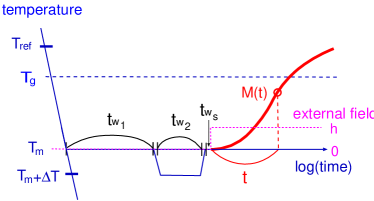
Figure 13: (Color online) Schematic representation of a one-step temperature cycling experiments according to the protocol $T_{\rm m}(t_{\rm w_{1}})\to T_{\rm m}+\Delta T(t_{\rm w_{2}})\to T_{\rm m}$. When returning to $T_{\rm m}$ a short waiting time $t_{\rm ws}=3$ s is needed, before applying the magnetic field and recording the ZFC relaxation, in order to ensure thermal stability. In ac experiments $\chi(t)$ is also recorded during the cycling.

In a one-step temperature cycling experiments (see Fig. 13), the sample is first cooled to $T_{\rm m}$ and aged there a time $t_{\rm w_{1}}$, the temperature is subsequently changed to $T_{\rm m}+\Delta T$ where the sample is aged for a time $t_{\rm w_{2}}$ (perturbation stage) and then the temperature is put back to $T_{\rm m}$ (healing stage). After a short wait time $t_{\rm ws}$ to ensure thermal stability at $T_{\rm m}$, the magnetic field is switched on and the magnetization $M_{\rm ZFC}(t)$ is recorded, or the ac susceptibility is recorded continuously during the cycling process.

A negative one-step $T$-cycling experiments ($\Delta T=-2$ K) measuring the out of phase component of the ac susceptibility is shown in Fig. 4. Results of such measurements with $t_{\rm w_{1}}=3000$ s are shown in Fig. 14. The aging at $Tm+\Delta T$ has been cut away in this figure and only the aging at $T_{\rm m}$ is shown. It can be clearly seen that the aging at $T_{\rm m}+\Delta T$ introduces a considerable amount of excessive response, which increases with increasing $t_{\rm w_{2}}$. In the ghost domain scenario the excessive response is attributed to the introduction of noise in the ghost domains by the aging at the temperature $T+\Delta T$. This yields a reduction of the order parameter [c.f. Eq. 17] so that the recovery time $t_{\rm rec}$ corresponds to the time scale at which the order parameter is recovered and hence the excessive susceptibility disappears [c.f. Eq. 20]. From Fig. 14, the recovery times $t_{\rm rec}$ are found to be of order $O(10^{3}-10^{4})$ s. If the $T$-cyclings would have kept the system in the weakly perturbed regime, the recovery times would become $t_{\rm rec}^{\rm weak}=0.04,\;0.1,\;0.3,\;0.9$ s for $t_{\rm w_{2}}=30,\;300,\;3000,\;30\,000$ s according to Eq. (15) and the growth law Eq. (28) with the same parameters as in Sec. IV.1.4. Consistent with the prediction in Sec. II.5.2, the observed values of $t_{\rm rec}$ are several orders of magnitude larger than $t_{\rm rec}^{\rm weak}$. However, the $t_{\rm w_{2}}$ dependence of $t_{\rm rec}$ is weaker than expected from Eq. 20, indicating that corrections to the assymptotic formula are important on the experimental length scales.foot_trec Finally, let us note that a similar observation of anomalously large recovery times was made in a recent study by Sasaki et al.sasetal2002

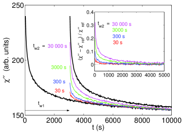
Figure 14: (Color online) $\chi^{\prime\prime}(t)$ vs time at $T_{\rm m}$ for experiments with a negative T-cycling of $\Delta T=-2$ K ($T_{\rm m}+\Delta T$ = 28 K); $t_{\rm w_{1}}$ = 3000 s and $t_{\rm w_{2}}$ = 30, 300, 3000, 30 000 s (bottom to top). The thick (black) lines represent the reference isothermal aging at $T_{\rm m}$, one of these curves is shifted a quantity $t_{\rm w_{1}}$ in time. The inset shows $[\chi^{\prime\prime}(t)-\chi^{\prime\prime}_{\rm ref}(t)]/\chi^{\prime\prime}_{\rm ref}(t)$ for the transient part of the susceptibility after the $T$-cycling. $\chi^{\prime\prime}(t)$ during the all stages of the $T$-cycling are shown in Fig. 4 for $t_{\rm w_{2}}=3000$ s. $\omega/2\pi=510$ mHz.

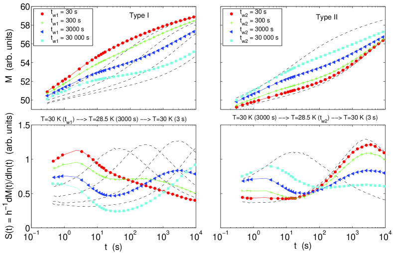
Figure 15: (Color online) ZFC relaxation curves ($M_{\rm ZFC}(t)$ and $S(t)$) obtained after a negative $T$-cycling of $\Delta T$ = -1.5K ($T_{\rm m}$ = 30 K; $T_{\rm m}+\Delta T$ = 28.5 K); Type I: $t_{\rm w_{1}}$ = 30, 300, 3000, and 30 000 s and $t_{\rm w_{2}}$ = 3000 s; Type II: $t_{\rm w_{1}}$ = 3000 s and $t_{\rm w_{2}}$ = 30, 300, 3000, 30 000 s. Isothermal aging recorded at $T_{\rm m}$ = 30 K are added for comparison in dashed lines; Type I: $t_{\rm w}$ = $t_{\rm w_{1}}$; Type II: $t_{\rm w}$ = 3 s and $t_{\rm w}$ = 3000 s. (See later Fig. 18 for the corresponding data of the one-step bond-cycling in the 4d EA model.)

The ZFC magnetization has been measured after negative one-step $T$-cyclings on the Ag(11 at% Mn) sample with $T_{\rm m}=30$ K and $\Delta T=-1.5$ K. Figure 15 shows the ZFC relaxation data; Type I: the initial wait time $t_{\rm w_{1}}$ is varied while the duration of the perturbation $t_{\rm w_{2}}=3000$ s is fixed. Type II: the initial wait time is fixed to $t_{\rm w_{1}}=3000$ s while the duration of the perturbation $t_{\rm w_{2}}$ is varied. Isothermal aging data are also shown in these figures for comparison. As seen in the figures, the magnetization always exhibits an enhanced growth rate at observation times around $t_{\rm min}$ after the cycling and in addition a second enhanced growth rate at observation times around $t_{\rm w_{1}}$ which are manifested as two peaks in the relaxation rate $S(t)$. The peak of $S(t)$ around $t_{\rm min}$ can be attributed to rejuvenation effects and the peak around $t_{\rm w_{1}}$ to memory effects. It can be seen that by increasing the duration of the perturbation $t_{\rm w_{2}}$ the height of the 2nd peak of $S(t)$ at around $t_{\rm w_{1}}$ dramatically decreases, but the peak position itself does not change appreciably. By studying the magnetization curve and comparing it to the reference curve of isothermal aging (with wait time $t_{\rm w}=t_{\rm w_{1}}$), it can be appreciated that the cycling data eventually merges with that of the isothermal aging curve (although it is outside the time scales of our measurements). The time scale of the merging appears to become larger for longer duration of the perturbation $t_{\rm w_{2}}$.

Within the ghost domain picture discussed in Sec. II, this two stage enhancement of the relaxation rate can be understood as follows. The aging at the second stage introduces strong noise and reduces the amplitude of the order parameter in the ghost domains $L_{T_{\rm m}}(t_{\rm w_{1}})$ grown at $T_{\rm m}$ during the initial aging. The system is hence strongly disordered with respect to the equilibrium state at $T_{m}$, but the original domain structure is conserved as a bias effect (the order parameter $\rho_{\rm rem}>0$). During the third stage (healing stage) the aging called inner-coarsening starts, i.e. new domain growth starting from an almost random state although with weakly biased initial condition. Hence, when the magnetic field is switched on in the healing stage, the inner-coarsening has already proceeded for the time $t_{\rm min}$. This is reflected by the 1st peak of $S(t)$. During the healing stage, the strength of the bias keeps increasing so that the noise (minority phases) within ghost domains is progressively removed. The 2nd peak of $S(t)$ corresponds to the size of the ghost domain $L_{T_{\rm m}}(t_{\rm w_{1}})$, which itself continues to slowly expand in the healing stage (outer-coarsening). Thus, this represents the memory of the thermal history before the perturbation. An illustration of this noise-imprinting-healing scenario is given in Fig. 3. However, the increase of the bias is so slow that the recovery time $t_{\rm rec}^{\rm strong}$ of the order parameter can be extremely large as given in Eq. (20). Then, the order parameter within a ghost domain may not be recovered fully until the ghost domain itself has grown appreciably in the healing stage. Probably this explains the fact that the 2nd peak of $S(t)$ is greatly suppressed (but not erased) by increasing the duration of the perturbation $t_{\rm w_{2}}$, which also increases the recovery time $t_{\rm rec}^{\rm strong}$.

V.1.2 Two-step temperature-cycling

Finally, two-step $T$-cyclings are studied in order to investigate the anomalous multiplicative effects of noise anticipated by the ghost domain picture [see Sec. II.5.3]. In this protocol an extra $T$-shift is added to the one-step temperature cycling procedure shown in Fig. 13; the sample is cooled to $T_{\rm m}$ where it is aged a wait time $t_{\rm w_{1}}$ (initial aging stage), subsequently the temperature is shifted to $T_{1}=T_{\rm m}+\Delta T_{1}$ for a time $t_{\rm w_{2}}$ (1st perturbation stage), then shifted to $T_{2}=T_{\rm m}+\Delta T_{2}$ for a time $t_{\rm w_{3}}$ (2nd perturbation stage) and finally changed back to $T_{\rm m}$ (healing stage) where $M_{\rm ZFC}(t)$ is recorded. As illustrated in Fig. 16 one can make two different kinds of 2-step-$T$-cycling experiments (with $T_{1},T_{2}<T_{\rm m}$); involving either a positive ($T_{2}>T_{1}$) or a negative ($T_{2}<T_{1}$) $T$-shift between $T_{1}$ and $T_{2}$.

Figure 16: Schematic illustration of a) positive ($T_{2}>T_{1}$) and b) negative ($T_{2}<T_{1}$) two-step-T-cycling.

In Fig. 17, a set of data using the two-step temperature-cycling protocol with $T_{\rm m}=30$ K and $t_{\rm w_{1}}=t_{\rm w_{2}}=t_{\rm w_{3}}=3000$ s are shown, together with reference data for one-step cycling experiments and isothermal aging experiments at $T_{\rm m}$. It can be seen that the data of the N-two-step experiment with $(T_{1},T_{2})=(29\,{\rm K},27\,{\rm K})$ is slightly more rejuvenated than the corresponding one-step cycling with $T_{\rm m}+\Delta T=29$ K and $t_{\rm w_{2}}=3000$ s, while the data of the P-two-step experiment with $(T_{1},T_{2})=(27\,{\rm K},29\,{\rm K})$ is much more rejuvenated. Furthermore, the data of the P-two-step experiment with $(T_{1},T_{2})=(28\,{\rm K},29\,{\rm K})$ is strikingly more rejuvenated, so that the $M_{\rm ZFC}(t)$ curve is close the one-step cycling with $T_{\rm m}+\Delta T=29$ K and $t_{\rm w_{2}}=30\,000$ s. This may appear surprising, since the total duration of the actual perturbation is only $t_{\rm w_{2}}+t_{\rm w_{3}}=6000$ s.

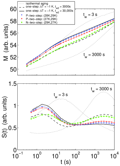
Figure 17: (Color online) ZFC relaxation curves obtained after negative two-step $T$-cyclings. Two-step-$T$-cycling experiments $T_{m}(t_{\rm w_{1}})\to T_{1}$ $(t_{\rm w_{2}})\to T_{2}$ $(t_{\rm w_{3}})\to T_{m}$ with $T_{m}=30$ K and $t_{\rm w_{1}}=t_{\rm w_{2}}=t_{\rm w_{3}}=3000$ s are shown. A negative $T$-shift in $T_{1}\to T_{2}$ is made with $(T_{1},T_{2})=(29\,{\rm K},27\,{\rm K})$ (diamonds), and positive $T$-shifts in $T_{1}\to T_{2}$ are made with $(T_{1},T_{2})=(28\,{\rm K},29\,{\rm K})$ (circles), $(T_{1},T_{2})=(27\,{\rm K},29\,{\rm K})$ (pulses). The isothermal aging with $t_{\rm w}=3$ and $3000$ s (dotted lines) at $T_{m}=30$ K and one-step $T$-cycling experiments $T_{m}(t_{\rm w_{1}})\to T_{\rm m}+\Delta T$ $(t_{\rm w_{2}})\to T_{m}$ with $T_{m}=30$ K, $T_{\rm m}+\Delta T=29$ K, $t_{\rm w_{2}}=3000$ and $30\,000$ s (dashed lines) are shown for comparison. (See Fig. 19 for the corresponding data of the two-step bond-cycling in the 4d EA model.)

The anomalously strong rejuvenation effect after the 2-step cycling can be understood by the ghost domain picture as the multiplicative effect of noise given in Eq. (22). One should however take into account the renormalization of the overlap length $L_{\Delta T}\to L_{\rm min}(v_{T},T)$ due to finiteness of heating/cooling rates discussed in Sec. II.6. Naturally, the latter effect can significantly or even completely hide the multiplicative nature of the noise introduction as appears to have happened in a previous study.bouetal2001 To reduce such “disturbing” effects as much as possible, one should use fast enough heating/cooling rates. It should also be recalled that in the present experiments, the heating is almost $10$ times faster than cooling which implies that the renormalized overlap length $L_{\rm min}(v_{T},T)$ is larger for cooling than for heating. This may explain the apparent asymmetry of the negative and positive two-step $T$-cyclings in Fig. 17. The weaker rejuvenation effect observed in the P-two-step measurement $(T_{1},T_{2})=(27\,{\rm K},29\,{\rm K})$ compared with $(28\,{\rm K},29\,{\rm K})$ can simply be attributed to the temperature dependence of the domain growth law Eq. (28).

V.2 Bond-cycling simulations

V.2.1 One-step bond cycling

For a one-step bond-cycling simulation on the $\pm J$ EA model, we prepare two sets of realizations of interaction bonds ${\cal J}^{A}$ and ${\cal J}^{B}$ as before. The set of bonds ${\cal J}_{B}$ is created from ${\cal J}_{A}$ by changing the sign of a small fraction $p$ of the latter randomly. In order to work in the strongly perturbed regime we choose $p=0.2$, since the analysis in the previous section (see Fig. 12) ensures that almost the whole time window of the simulations lies well within the strongly perturbed regime with $p=0.2$. We also made simulations with weaker strength of the perturbation $p=0.05$, for which time scales greater than $10^{3}$ MCS belongs to the strongly perturbed regime as can be seen in Fig. 12, and obtained qualitatively the same results but with larger statistical errors. The working temperature is fixed to $T/T_{g}=0.6$ throughout the simulations and the strength of the probing field is $h/J=0.1$, which is small enough to observe linear response within the present time scales.yoshuktak2002

The procedure of the one-step bond-cycling is the following. First the system is let to evolve under ${\cal J}^{A}$ for a time $t_{\rm w_{1}}$ at temperature $T$ starting from a random spin configuration. Then, the bonds are replaced by ${\cal J}^{B}$ and the system is let to evolve another time interval $t_{\rm w_{2}}$. Finally, the bonds are put back to ${\cal J}^{A}$ and the system is let to evolve. After a time interval $t_{\rm w_{3}}$, a small magnetic field $h$ is switched on and the growth of the magnetization is measured to obtain the ZFC susceptibility

$$\chi_{\rm ZFC}(t)=(J/h)(1/N))\sum_{i}\langle S_{i}(t+t_{\rm w_{3}}+t_{\rm w_{2}}+t_{\rm w_{1}})\rangle$$ (25)

where $t$ is the time elapsed after the magnetic field is switched on. We also measured the conjugate auto-correlation function to the ZFC susceptibility in the same protocol but without applying a magnetic field,

$$C_{\rm ZFC}(t)=C(t+t_{\rm w_{3}}+t_{\rm w_{2}}+t_{\rm w_{1}},t_{\rm w_{3}}+t_{\rm w_{2}}+t_{\rm w_{1}}),$$ (26)

where $C(t_{1},t_{2})=(1/N)\sum_{i}S_{i}(t_{1})S_{i}(t_{2})$ is the spin autocorrelation function. Again, the subscript “ZFC” is put to emphasize that this auto correlation function is conjugate to the ZFC susceptibility if the FDT holds. We expect both quantities to reflect the inner- and outer-coarsening discussed in Sec. II, but there are also apparent differences. Firstly, the FDT is expected to be violated in the outer-coarsening regime.yoshuktak2002 Secondly, the linear susceptibility $\chi_{\rm ZFC}(t)$ should have the so called weak long term memory (WLTM) property bouetal97 , stating that an integral of linear responses during a finite interval of time finally disappears at later times, whereas the auto correlation does not have such a property.

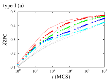
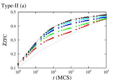
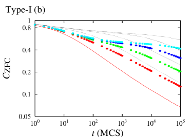
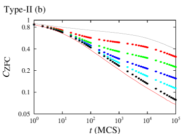
Figure 18: (Color online) ZFC susceptibility and the corresponding auto-correlation function in the 4DEA model after bond-cyclings. The filled squared are the data obtained after bond-cyclings with Type I: $t_{\rm w_{1}}=10^{2},10^{3},10^{4},10^{5}$ (MCS) ($\chi_{\rm ZFC}$ from top to bottom $C_{\rm ZFC}$ from bottom to top), $t_{\rm w_{2}}=10$, and $t_{\rm w_{3}}=10$ (MCS); Type II: $t_{\rm w_{1}}=10^{4}$ (MCS), $t_{\rm w_{2}}=10,40,160,640$ and $10^{5}$ (MCS) ($\chi_{\rm ZFC}$ from top to bottom $C_{\rm ZFC}$ from bottom to top), and $t_{\rm w_{3}}=10$ (MCS). The solid lines are the reference isothermal aging data (a) $\chi_{0}(t,t_{\rm w})$ (b) $C_{0}(t,t_{\rm w})$ with $t_{\rm w}=t_{\rm w_{3}}$ and the dotted lines those with $t_{\rm w}=t_{\rm w_{1}}+t_{\rm w_{3}}$. (See Fig. 15 for the corresponding temperature-cycling experiment.)

In Fig. 18, we show a data set labeled “type-I”, where the initial wait time $t_{\rm w_{1}}$ is varied while the other time scales are fixed. Another data set labeled “type-II” is also shown, where the duration of the perturbation $t_{\rm w_{2}}$ is varied while the other time scales are fixed. The corresponding data in the case of temperature-cyclings are shown in Fig. 15. In all data in Fig. 18, there is a common feature that the ZFC susceptibility $\chi_{\rm ZFC}(t)$ and the conjugate auto correlation function $C_{\rm ZFC}(t)$ exhibit two-step relaxation processes which can be naturally understood as the inner- and outer-coarsening discussed in section II. In the figures the data of the reference isothermal aging without perturbations of the ZFC susceptibility $\chi_{0}(t,t_{\rm w})$ and the autocorrelation function $C_{0}(t,t_{\rm w})$ are shown for comparison.

Quite remarkably, the generic features of the behavior of the ZFC susceptibility $\chi_{\rm ZFC}(t)$ is the same as in temperature-cycling experiments. First, there is an initial growth of the susceptibility which appears to be close to the curve of the reference isothermal aging $\chi_{0}(t,t_{\rm w})$ with wait time $t_{\rm w}=t_{\rm w_{3}}$. This feature can be naturally understood to be due to the inner-coarsening. Then, there is a crossover to $\chi_{0}(t,t_{\rm w})$ with wait time $t_{\rm w}=t_{\rm w_{1}}+t_{\rm w_{3}}$ which can naturally be understood to be due to the outer-coarsening.

Correspondingly, and as expected, the auto-correlation function $C_{\rm ZFC}(t)$ exhibits a similar two-step relaxation as $\chi_{\rm ZFC}(t)$. It initially follows the reference curve $C_{0}(t,t_{\rm w})$ of $t_{\rm w}=t_{\rm w_{3}}$ (inner-coarsening) and makes a crossover to slower decay which depends on $t_{\rm w_{1}}+t_{\rm w_{3}}$ (outer-coarsening) at later times. This auto-correlation function was studied in bond-cycling simulations of the spherical and Ising Mattis model in Ref. yoslembou2001, with rejuvenation put in by hand, where essentially the same result as here was obtained. Thus, the present results support that the same mechanism of memory is at work in the spin-glass model.

V.2.2 Two-step bond-cycling

For the two-step bond-cycling, we consider that the procedure ${\cal J}^{A}\to{\cal J}^{B}\to{\cal J}^{C}\to{\cal J}^{A}$ is the same as the one-step bond cycling except that some time $t_{\rm w_{3}}$ is spent at ${\cal J}^{C}$ before coming back to ${\cal J}^{A}$. The bonds of ${\cal J}^{A}$ and ${\cal J}^{B}$ are prepared as in the one-step cycling case, i.e the set of bonds ${\cal J}^{B}$ is created from ${\cal J}^{A}$ by a perturbation of strength $p$. The 3rd set of bonds ${\cal J}^{C}$ is created from ${\cal J}^{B}$ by a perturbation of strength $p$. Note, that this corresponds to create ${\cal J}^{C}$ out of ${\cal J}^{A}$ by a perturbation of strength $p^{\prime}=2p(1-p)$. Here, we again use $p=0.2$ and thus $p^{\prime}=0.32$ in order to work in the strongly perturbed regime. The temperature is again fixed to $T/T_{g}=0.6$ throughout the simulations and the strength of the probing field is $h/J=0.1$.

In Fig. 19, we show the ZFC susceptibility $\chi_{\rm ZFC}(t)$ and the conjugate auto correlation function $C_{\rm ZFC}(t)$ after the two-step bond cyclings ${\cal J}^{A}\to{\cal J}^{B}\to{\cal J}^{C}\to{\cal J}^{A}$ which is compared with the data of one-step bond cyclings ${\cal J}^{A}\to{\cal J}^{C}\to{\cal J}^{A}$. It can be seen that the effect of the two step perturbations with $t_{\rm w_{2}}=t_{\rm w_{3}}=10$ (MCS) is stronger than the one step perturbation with $t_{\rm w_{2}}=20$ (MCS). Moreover, two step perturbations with $t_{\rm w_{2}}=t_{\rm w_{3}}=80$ (MCS) is as strong as the one step perturbation with $t_{\rm w_{2}}=640$ (MCS).

The above result can hardly be understood by a naive length scale argument. It resembles the result of the corresponding two-step temperature cycling experiments discussed in Sec. V.1 and is consistent with the expectation in the ghost domain scenario, which predicts multiplicative effects of perturbations in the strongly perturbed regime (see Eq. (22)).

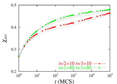
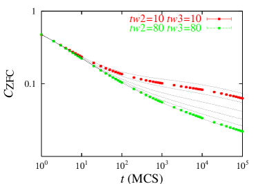
Figure 19: (Color online) The relaxation after two-step bond-cycling ${\cal J}^{A}\to{\cal J}^{B}\to{\cal J}^{C}\to{\cal J}^{A}$. The target equilibrium state is cycled as ${\cal J}^{A}$ ($10^{4}$ (MCS)) $\to$ ${\cal J}^{B}$ ($t_{\rm w_{2}}$ (MCS)) $\to$ ${\cal J}^{C}$ ($t_{\rm w_{3}}$ (MCS)) $\to$ ${\cal J}^{A}$ ($t$ (MCS)). In the figures the dotted lines are the reference data of one-step bond-cycling ${\cal J}^{A}$ ($10^{4}$ (MCS)) $\to$ ${\cal J}^{C}$ ($t_{\rm w_{2}}$ (MCS)) $\to$ ${\cal J}^{A}$ ($t$ (MCS)) with $t_{\rm w_{2}}=20,40,80,160,320,640$ (MCS) which vary from bottom to top in (a) and from top to bottom in (b). (See Fig. 17 for the corresponding two-step temperature-cycling experiment.)

VI Memory experiments

This section discusses memory experiments, which probes nonequilibrium dynamic under continuous temperature changes and halts, using low frequency ac susceptibility and ZFC magnetization measurements. Such experiments have become a popular tool for investigations of memory and rejuvenation effects in various glassy systems, for example interacting nanoparticles,jonhannor2000 polymer glasses,belcillar2002 and granular superconductorsgaretal2003 . It can however be difficult to interpret the experiments, since memory and rejuvenation effects are mixed with cooling/heating rate effects in a nontrivial way.

VI.1 ac memory

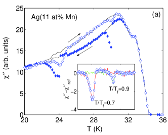
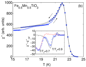
Figure 20: (Color online) $\chi^{\prime\prime}$ vs temperature with temporary stops at (a) $T_{\rm s_{1}}$ = 30 K and $T_{\rm s_{2}}$ = 24 K and (b) $T_{\rm s_{1}}$ = 20 K and $T_{\rm s_{2}}$ = 16 K; $t_{s_{1}}=t_{s_{2}}$ = 3000 s. These values of $T_{\rm s}$ correspond to $T/T_{\rm f}=0.9$ and 0.7 for both samples, where $T_{\rm f}$ is the freezing temperature.foot_Tf Filled symbols are used to represent the curves measured on cooling, and open symbols the curves measured on heating. The reference curves (without stops) are shown as lines, the arrows indicate the cooling respective the heating curve. The insets show the difference plots for double stop experiments (open symbols) and associated single stop experiments (lines) measured on heating. $\omega/2\pi$ = 510 mHz and $v_{\rm cool}^{\rm eff}\approx v_{\rm heat}^{\rm eff}\sim 0.005$.

Results of ac-susceptibility memory experiments are shown in Fig. 20; the ac susceptibility is measured on cooling and on the subsequent reheating. Measurements are made both with and without temporary stop(s) at constant temperature on cooling. In the figure, $\chi^{\prime\prime}(T)$ is plotted vs. temperature for the two samples. It is interesting to note that even without a temperature stop, we observe differences between Ag(11 at% Mn) and Fe_0.5Mn_0.5TiO₃ as regard the relative levels of $\chi^{\prime\prime}(T)$ measured on cooling and reheating (the ”direction” of measurement is indicated with arrows on the figure). In the case of Ag(11 at% Mn) , the heating curve lies significantly above the cooling curve (except close to the lowest temperature). Such a behavior can only be explained by strong rejuvenation processes during the cooling and reheating procedure. In the case of Fe_0.5Mn_0.5TiO₃ , on the other hand, the susceptibility curve recorded on reheating lies below the corresponding cooling curve, indicating that some equilibration of the system is accumulative in the cooling/reheating process. By making one or two temporary stops during the cooling processes, memory dips are introduced in the susceptibility curves on reheating as seen in the main frames and illustrated as difference plots in the insets of Fig. 20. These figures illustrate one more marked differences in the behavior of the two samples: the memory dips are wider for the Fe_0.5Mn_0.5TiO₃ than for the Ag(11 at% Mn) sample.

VI.2 ZFC memory

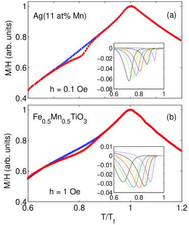
Figure 21: (Color online) ZFC susceptibility vs $T/T_{\rm f}$ for (a) the Ag(11 at% Mn) sample and (b) the Fe_0.5Mn_0.5TiO₃ sample. The ZFC susceptibility is measured after continuous cooling (filled symbols) and cooling with a temporary stop (open symbols) of 3000 s at $T_{\rm s}/T_{\rm f}$ $\sim$ 0.8 ($T_{\rm s}$ = 27 K for Ag(11 at% Mn) and $T_{\rm s}$ = 19 K for Fe_0.5Mn_0.5TiO₃ ). The insets show the corresponding difference plots (”stop curve” - reference curve), and additional results for 3000 s stops made at (a) $T_{\rm s}$ = 24-31 K and (b) $T_{\rm s}$ = 16-21 K. $v_{\rm cool}\sim 0.05$ K/s and $v_{\rm heat}^{\rm eff}\sim 0.005$.

ZFC memory experiments matetal2001 ; matetal2002 will here be used to further elucidate the differences between the two samples. Results of single stop ZFC memory experiments for the Ag(11 at% Mn) and Fe_0.5Mn_0.5TiO₃ spin glasses are shown in Fig. 21. In both cases, the sample is cooled in zero magnetic field and the cooling is temporary stopped at $T_{\rm s}/T_{\rm f}$ = 0.8 for $t_{\rm s}$ = 3000 s (main frame). Here $T_{\rm f}$ is the freezing temperature of the ZFC magnetization.foot_Tf The cooling is subsequently resumed and the ZFC magnetization recorded on reheating in a small magnetic field. A reference curve measured using the same protocol but without the stop is also recorded. The difference between corresponding reference and single memory curves are plotted in the inset, together with results obtained from similar measurements with stops at some other temperatures. As seen in the main frames, the curves corresponding to the single stops lie significantly below their reference curves in a limited temperature range around $T_{\rm s}/T_{\rm f}$. In the associated difference plots, this appears as ”dips” of finite width around the stop temperatures. It has been argued that such dips directly reflect the memory phenomenon.matetal2001

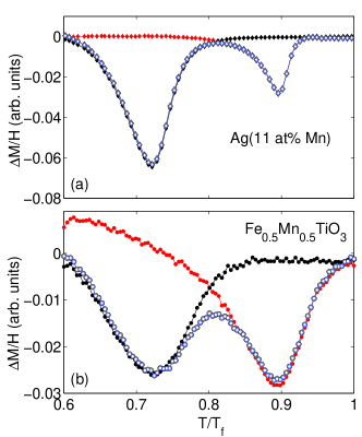
Figure 22: (Color online) Difference plots of ZFC susceptibility vs $T/T_{\rm f}$ corresponding to single and double stop experiments, with one (or two) temporary stops for 3000 s at (a) $T_{s_{1}}$ = 30 K or/and $T_{s_{2}}$ = 24 K and (b) $T_{s_{1}}$ = 21 K or/and $T_{s_{2}}$ = 17 K. The single stop experiments are represented using filled markers, while open markers are used to represent the double stops experiments. $v_{\rm cool}\sim 0.05$ K/s and $v_{\rm heat}^{\rm eff}\sim 0.005$.

The memory dips appear much broader for the Fe_0.5Mn_0.5TiO₃ sample than for the Ag(11 at% Mn) sample. This can be seen even more clearly in the double stop dc-memory experiments shown in Fig. 22. Two 3000 s stops are performed at $T_{\rm s_{1}}/T_{\rm f}$ = 0.9 and $T_{\rm s_{2}}/T_{\rm f}$ = 0.72 during the cooling to the lowest temperature. The results of the corresponding single stop experiments at $T_{\rm s_{1}}$ and $T_{\rm s_{2}}$ are included. For both systems, the sum of the two single stop curves (not shown here) is nearly equal to the double stop curve.matetal2002 But, while for Ag(11 at% Mn) the two peaks are well separated, for the same separation in $T/T_{\rm f}$, the single stop curves of Fe_0.5Mn_0.5TiO₃ overlap, due to the larger width of the memory dips.

VI.3 Accumulative vs chaotic processes

In the ghost domain picture, the size of domains at a given temperature $T$ can be increased by aging at nearby temperatures (see Fig. 2). However, noise is induced on the domains at $T$ by the growth of domains at other temperatures outside the overlap region (c.f. Sec. II.5.2). In particular the spin configuration subjected to continuous temperature changes with a certain rate $v_{T}$ is expected to attain a domain size $L_{\rm min}(v_{T},T)$ at temperature $T$, due to the competition between accumulative aging and chaotic rejuvenation processes (as discussed in Sec. II.6). $L_{\rm min}(v_{T},T)$ is reflected on the magnetic response of the systems under continuous temperature changes; the larger $L_{\rm min}(v_{T},T)$ the smaller $\chi^{\prime\prime}(T)$. In the data of the ac susceptibility measured under continuous cooling and reheating shown in Fig. 20, we found that for the Ag(11 at% Mn) sample the $\chi^{\prime\prime}(T)$ curve on reheating lies above the one measured on cooling, while the opposite applies to the Fe_0.5Mn_0.5TiO₃ sample. These features suggest strong chaotic rejuvenation in Ag(11 at% Mn) and much weaker in the Fe_0.5Mn_0.5TiO₃ sample. This is qualitatively consistent with the observations made in the temperature-shift experiments presented in Sec. IV.1 that the overlap length for the Ag(11 at% Mn) decays faster with increasing $\Delta T$ than that of the Fe_0.5Mn_0.5TiO₃ system.

VI.4 An apparent hierarchy of temperatures

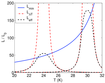
Figure 23: (Color online) A schematic illustration of the length scales explored in the Ag(11 at% Mn) sample by continuous cooling (and heating) with temporary halts at $T_{s1}=30$ K and $T_{s2}=24$ K for $t_{s1}=t_{s2}=10^{4}$ s. The effective domain size grown during the temporary halts at $T_{s}$ for a time $t_{s}$ is given by $L_{\rm eff}=L_{\Delta T=|T-T_{s}|}F(L_{T_{s}}(t_{s})/L_{\Delta T=|T-T_{s}|})$ [Eq. (9-12)]. It is bounded from above by the overlap length $L_{\Delta T=|T-T_{s}|}$. The scaling function $F(x)=\tanh(x)(1-cx^{2\zeta}/\cosh(x))$ interpolates between the fit to the weakly perturbed regime (shown in Fig. 10) and the strongly perturbed regime $\lim_{x\to\infty}F(x)=1$. Here all parameters for the growth law $L_{T}(t)$ [see Fig. 24] and the overlap length $L_{\Delta T}$ are the same as in Sec. IV.1.4. The continuous cooling and heating yields the minimum effective domain size $L_{\rm min}$ at all temperatures. Here it is simply assumed to be $L_{\rm min}=L_{T}(t_{\rm min})$ with $t_{\rm min}=100$ s.foot_lmin

In a memory experiment, during a stop made at $T_{s}$ for a time $t_{\rm s}$ the size of the domains becomes $L_{T_{\rm s}}(t_{\rm s})$. The ghost domains at nearby temperatures will also grow but only up to $L_{\rm eff}$ [Eq. (9)], as illustrated in Fig. 23. The min($L_{T_{s}}(t_{w}),L_{\Delta T=|T_{s}-T|}$) is the upper bound for $L_{\rm eff}$. When the cooling is resumed, the ac susceptibility curve merges with the reference curve because the overlap length becomes smaller than the minimum domain size $L_{\rm min}$, which depends on the cooling rate.foot_lmin On the subsequent reheating the domain sizes at the temperatures around $T_{\rm s}$ are larger than $L_{\rm min}$ so that the susceptibility curve (ac or dc) measured on heating makes a “dip” with respect to the reference curve without any stop.

Let us compare the schematic picture of length scales for the Ag(11 at% Mn) sample shown in Fig. 23 with the corresponding 2-stop memory experiment shown in Fig. 20 and 22. We can see that the widths of the dips around $T_{s}$ in the memory experiment correspond roughly to the widths of the temperature-profile of the effective domain size $L_{\rm eff}$ at around $T_{s}$. The width of the memory dips becomes broader at lower temperatures for all memory experiments both for the Ag(11 at% Mn) and Fe_0.5Mn_0.5TiO₃ samples. In the length scale picture it is also seen that the temperature profile of $L_{\rm eff}$ around $T_{s}$ becomes broader at lower temperature, due to the temperature dependence of the growth law (see Fig. 24). From this scenario it is clear that a larger overlap length makes the weak chaos regime larger and hence the memory dips broader. The observed differences between the width of the dips of the Fe_0.5Mn_0.5TiO₃ and Ag(11 at% Mn) samples may be attributed to such a difference in overlap length in consistency with the results shown in Fig. 9.

The distinct multiple memories shown in Figs. 20 and 22 could suggest some sort of “hierarchy of temperatures”. However, it is not necessary to invoke neither the traditional hierarchical phase space picture vinetal96 nor the hierarchical length scale picture komyostak2000A ; bouchaud2000 ; bouetal2001 ; berbou2002 ; berhol2002 ; takhuk2002 ; beretal to understand this multiple memory effect. Indeed, the domain sizes grown at the two stop temperatures are almost of the same order of magnitude since thermally activated dynamics does not allow significant hierarchy of length scales explored at different temperatures (as discussed in Appendix A). Thus the scenarios of the memory effect which strongly relies on the assumption of hierarchy of length scales komyostak2000A ; bouchaud2000 ; bouetal2001 ; berbou2002 ; berhol2002 ; takhuk2002 ; beretal cannot explain the distinct memory dips. Without temperature-chaos, the temperature profile of $L_{\rm eff}$ becomes so broad that the memory dips strongly overlap. Our estimates suggest that the sizes of domains grown at the two stop temperatures shown in Fig. 23 are much larger than the overlap length between the equilibrium spin configurations at the two temperatures within the experimental time scales. Thus the memories imprinted at the two stop temperatures are significantly different from each other. Also, retrieval of such memories under strong temperature-chaos effect is possible within the ghost domain picture as discussed in Sec II.5. A crucial ingredient in experiments is the finiteness of the heating and cooling rate which yields the characteristic length scale $L_{\rm min}$, schematically shown in Fig. 23. As discussed in section Sec. II.6, $L_{\rm min}$ plays the role of a renormalized overlap length which leads to substantial reductions of the recovery times of memories.

It should however be noted that much broader memory dips are observed in experimental systems such as superspin glasses, for which experiments probe short time (length) scales so that the effect of temperature-chaos is negligible, and the memory dip is determined by freezing of smaller and smaller domains on cooling in a fixed energy landscapejonetal2004 (see also Ref. bouetal2001, ). Lastly, we note that the width of the memory dips give an indication of the strength of the temperature-chaos effect, but a better estimation is given by the twin T-shift experiments discussed in Sec. IV.

VII Summary and conclusion

Rejuvenation (chaos) and memory effects have been investigated after temperature perturbations in two model spin glass samples, the Fe_0.5Mn_0.5TiO₃ Ising system and the Ag(11 at% Mn) Heisenberg system, as well as after bond perturbations in the 4 dimensional EA Ising model. These effects are discussed in terms of the ghost domain picture presented in Sec. II.

• The ZFC relaxation is measured after a $T$-shift for the Fe_0.5Mn_0.5TiO₃ and Ag(11 at% Mn) samples. By analyzing the peak positions of the relaxation rate $S(t)$ using the twin $T$-shift protocol introduced in Ref. jonyosnor2002, , evidences of both accumulative and non-accumulative aging regimes in both samples were found (cf. Fig. 9). The Ag(11 at% Mn) sample was found to exhibit stronger deviations from fully accumulative aging with increasing $|\Delta T|/T_{\rm g}$ than the Fe_0.5Mn_0.5TiO₃ sample. A scaling analysis, performed on the data of the Ag(11 at% Mn) sample (Fig. 10), reveals increasing rejuvenation effects with increasing $\Delta T$. These rejuvenation effects can consistently be understood in terms of partial chaos at length scales smaller than the overlap length $L_{\Delta T}$, as first proposed in Ref. jonyosnor2003, . However, data derived using larger perturbations $|\Delta T|>0.6$ K could not be used in the scaling analysis because the rejuvenation effect saturates due to the slow cooling/heating rates. This suggests the emergence of the strongly perturbed regime in the sense that $L_{\Delta T}<L_{\rm min}$, where $L_{\rm min}$ is the smallest observable domain size due to the slow cooling/heating. The overlap length can never be directly observed in experiments since it is hidden behind $L_{\rm min}$ as can be seen in the schematic Fig. 23. On the other hand some properties of the overlap length are obtained indirectly by the scaling in the weakly perturbed regime (Fig. 10).

• In the case of bond-shift simulations, the relaxation rate $S(t)$ is found to show a similar behavior as in the $T$-shift experiments as shown in Fig. 11; $S(t)$ is initially broadened with increasing strength of the perturbation $p$, where also the scaling analysis presented in Fig. 12 exhibits the emergence of corrections to the fully accumulative aging. The scaling ansatz Eq. (9-11) was shown to hold with only the chaos exponent $\zeta$ being a fitting parameter, a result that also gives further support to the corresponding analysis from $T$-cycling experiments. However, again the data with stronger perturbation (larger $p$) could not be used in the scaling because the peak positions saturated to $O(1)$ (MCS), which is the minimum time scale. In such a regime, $S(t)$ exhibits considerable narrowing with the peak at $O(1)$ (MCS). This can again be understood to be due to the emergence of the strongly perturbed regime in the sense that $L_{\Delta T}\sim L_{0}$ where $L_{0}$ is the unit of lattice spacing.

• For the Ag(11 at% Mn) sample temperature changes $|\Delta T|\gtrsim 1$ K were shown to cause strong perturbations to the system. One and two-step negative $T$-cycling protocols were used in order to investigate the healing after such strong perturbations. The recovery times after one-step cyclings shown in Figs. 15 and 14 were found to be anomalously larger than the trivial recovery times $t_{\rm rec}^{\rm weak}$ given in Eq. (15) (which could be evaluated using the growth law confirmed in Sec. IV.1.4). Furthermore, the two-step cyclings data displayed in Fig. 17 show that the effects of perturbations made at two different temperatures can give rise to much stronger rejuvenation than only an additive increase of the effects of single perturbations. These striking features are in agreement with ghost domain scenario (Sec. II.5).

• In the bond-cycling simulations, a large strength of the perturbation, $p=0.2$, was used to focus on the strongly perturbed regime. The healing process after one-step cycling simulations displayed in Figs. 18 and and the two-step bond-cycling shown in Fig. 19 were found to require anomalously large recovery times, in consistency with the results from $T$-cycling experiments and the predictions of the ghost domain scenario. It is also demonstrated in Fig. 19 that a “memory” of the history before the perturbation cannot be erased completely even if the duration of the perturbation is effectively longer than the duration of the preceding history.

• It is proposed that the effects of finite heating/cooling rates $v_{T}$ can be parameterized by a renormalized overlap length $L_{\rm min}(v_{T},T)$. In combination with a strong separation of time scales, this can lead to an apparent “hierarchy of temperatures”, as has been suggested earlier from experimental observations e.g. in Refs. ledetal91, ; lefetal92, . In the ghost-domain scenario however, the temperature chaos effect is the mechanism which allows distinctness of memories at each level of the “hierarchy” as illustrated in Fig. 23. This explains the two well separated memory dips seen in e.g. the memory experiment shown in Fig. 20.

To conclude, dynamical properties of the Ising Fe_0.5Mn_0.5TiO₃ and the Heisenberg Ag(11 at% Mn) spin glasses subjected to temperature changes and the 4 dimensional Edwards Anderson Ising spin glass model subjected to bond changes are examined and compared with each other in detail. The temperature-shift/cycling experiments and bond-shift/cycling simulations show remarkably similar features suggesting a common mechanism of the rejuvenation and memory effects. The detailed features of the rejuvenation effects after temperature/bond shifts are found to agree with the anticipated crossover from weakly to strongly perturbed regimes of the chaos effects. Quantitative differences in different systems can be attributed to differences of the magnitude of the overlap length. Anomalously large recovery times of the memories are found to be required in the one and two-step temperature/bond cycling experiments when performed into the strongly perturbed regime, in agreement with the ghost domain scenario.

Appendix A Separation of length and time scale

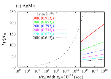
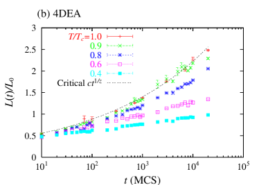
Figure 24: (Color online) The dynamical length scales relevant in our experiments and simulations. (a) A plot of the growth law Eq. (28) with parameters determined for a Ag(11 at% Mn) sample in Ref. jonetal2002PRL, from a scaling analysis of the relaxation of the ac susceptibility in isothermal aging in the range $20-30$ K. The growth law at the critical temperature $L(t)/L_{0}=(t/\tau_{m})^{1/z}$ ($z=6.5$) is also shown. (The possible $O(1)$ prefactor in front of Eq. (28) and the critical growth law is not known.) The unit of time is chosen to be $\tau_{\rm m}\sim\hbar/J\sim 10^{-13}$ s. The experimental time-length scale is the area surrounded by the box. (b) The size of the domains of a 4 dimensional EA Ising spin glass model determined directly in a previous numerical simulation hukyostak2000 monitoring the spatial correlation function between two real replicas undergoing isothermal aging. The dotted line is the power law for the critical regime $L(t)/L_{0}=(t/\tau_{m})^{1/z}$ with $z=4.98$.

In this appendix we summarize important properties of activated dynamics that governs the growth of domains in spin glasses. At mesoscopic levels, the dynamics of a spin glass at temperatures below $T_{g}$ is governed by nucleation of droplet like excitations.fishus88noneq The energy barrier associated with a droplet of size $L$ is assumed to scale as $E_{\rm b}\sim\Delta(T)(L/L_{0})^{\psi}$ with $\psi>0$. Then the time needed to nucleate a droplet by thermal activation becomes

$$\tau_{L}(T)=\tau_{0}(T)\exp\left[\frac{\Delta(T)}{k_{\rm B}T}\left(\frac{L}{L_{0}}\right)^{\psi}\right]$$ (27)

where the effects of critical fluctuations are taken into account in a renormalized way in the characteristic energy scale $\Delta(T)$ for the free-energy barrier and the characteristic time scale $\tau_{0}(T)$ for the thermally activated processes. They scale as $\Delta(T)/J\sim\epsilon^{\psi\nu}$ and $\tau_{0}(T)/\tau_{\rm m}\sim(\xi(T)/L_{0})^{z}\sim|\epsilon|^{-z\nu}$ with $\epsilon=T/T_{g}-1$. The microscopic time scale is $\tau_{\rm m}\sim\hbar/J\sim 10^{-13}$ s in atomic spin glasses and one Monte Carlo Step (MCS) in Monte Carlo simulations. $J\sim T_{g}$ sets the energy unit, $z$ is the dynamical critical exponent and $\nu$ the exponent for the divergence of the correlation length. The importance of accounting for critical fluctuations has been realized in analyzes of recent simulations hukyostak2000 ; berbou2002 ; yoshuktak2002 and experiments.bouetal2001 ; jonetal2002PRL

From Eq. (27) it follows that within a time scale $t$ a droplet excitation as large as

$$L_{T}(t)\sim L_{0}\left[\frac{k_{\rm B}T}{\Delta(T)}\ln\left(\frac{t}{\tau_{0}(T)}\right)\right]^{1/\psi}\,$$ (28)

can be thermally activated. At finite time scales there must be corrections to the asymptotic form Eq. (28) due to critical fluctuations bouetal2001 ; yoshuktak2002 as well as logarithmic correction terms to the energy barriers mikdrokar95 but the actual forms of the corrections are not yet known in spin-glasses.

An immediate consequence of activated dynamics is an extremely wide separation of time scales with temperature. On the other hand the variation of length scales with temperature is very mild (typically less than one order in magnitude). Let us consider two arbitrarily close temperatures $T$ and $T+\Delta T$. From Eq. (27) it follows that the ratio of time scales at the two temperatures associated with a given length $L$ for $\Delta T/T\ll 1$ becomes,

$$\frac{\tau_{L}(T)}{\tau_{L}(T+\Delta T)}\sim\frac{\tau_{0}(T)}{\tau_{0}(T+\Delta T)}\exp\left[\left(\frac{L}{L_{*}(\Delta T)}\right)^{\psi}\right]$$ (29)

where we introduced time-separation length

$$L_{*}(\Delta)\sim L_{0}\left|(\partial(\Delta(T)/k_{\rm B}T)/\partial T)\Delta T\right|^{-1/\psi}.$$ (30)

The above expression means that two times become exponentially separated if one observes dynamics on length scales large enough compared with the time-separation length $L_{*}(\Delta T)$. Note that $L_{*}(\Delta T)$ remains finite as long as $\Delta T$ is non-zero. Looking at the ratio of length scales for a given time scale $t$ at the two temperatures one finds from Eq. (28),

$$\frac{L_{T+\Delta T}(t)}{L_{T}(t)}\sim O(1)$$ (31)

independently of the chosen time scale $t$. Thus, the magnitude of the length scales explored at two close temperatures appears quite similar as long as the same time scales are used. However, we emphasize, that thermally activated dynamics brings about a significant hierarchy of time scales, in spite of an apparent mild hierarchy in length scales.

Assuming that Eq. (28) is applicable to the Heisenberg like Ag(11 at% Mn) spin glass, Fig. 24(a) shows the domain growth at different temperatures in this system using earlier derived experimental values for the parameters. jonetal2002PRL In Fig. 24(b) the domain growth at different temperatures is drawn for a 4d EA spin glass derived from previous numerical simulations. hukyostak2000

In spin glass materials the microscopic time is $\tau_{\rm m}\sim 10^{-13}$ s and relaxation experiments are performed typically in the range of time scales $1-10^{5}$ s or $t/\tau_{\rm m}=10^{13}-10^{18}$. On the other hand, in usual Monte Carlo simulations of EA Ising spin glass models the microscopic time is $\tau_{\rm m}=1$ Monte Carlo Step (MCS) and the range of time scales is $1-10^{6}$ (MCS) or $t/\tau_{\rm m}=1-10^{6}$. Because of the slow dynamics, there is a common problem that the investigated 4-6 decades in time only cover a quite limited length scale as shown in Fig. 24 (see also Fig 1 of Ref. berbou2002, ). Due to the much shorter time scales probed in numerical simulations, the influence of critical dynamics are much stronger than in experiments for the same reduced temperature $T/T_{\rm g}$. It can also be seen in Fig. 24 that the length scales are rather different: simulations explore length scales of order $L_{T}(t)/L_{0}\sim O(1)$ while experiments explore $L_{T}(t)/L_{0}\sim O(10)-O(10^{2})$.

Appendix B Experimental details

B.1 Non-commercial SQUID magnetometer

The experiments were performed in non-commercial SQUID magnetometers,magetal97 designed for low-field measurements and optimum temperature control. The magnetic field is in these set-ups generated by a small superconducting solenoid always working in persistent mode. The time constant of the superconducting magnets is of order 1 ms, but the whole procedure to change the field from $h$ to $h+\Delta h$ and re-establish persistent mode in the magnet takes $\sim$ 0.3 s which also determines the shortest observation time in the ZFC relaxation experiments. In the case of the Fe_0.5Mn_0.5TiO₃ sample, cut into a rectangular shape ($2\times 2\times 4$ mm³) with the c-axis along the longest side, the probing field was applied along the $c$-axis of the single crystal, and for the Ag(11 at% Mn) spin-glass, turned into a cylindrical shape (4 mm long and 2 mm in diameter), the field was applied along the symmetry axis of the cylinder. The sample space is magnetically shielded with cans of $\mu$-metal and niobium and the remaining background field is $<1$ mOe, while the measurement field used are $h\approx 0.1-1$ Oe. The sample is glued to a 50 mm long sapphire rod with a diameter of 2 mm, and the magnetization is recorded while keeping the sample stationary in the center of the third coil of a third order gradiometer. The sapphire rod is connected to a solid copper cylinder on which the thermometer and a resistive heater are placed. The materials in the experimental setup are chosen so that the heat transfer between the sample and copper cylinder is maximized while the heat exchange with the surroundings is kept quite low being mainly carried by thermal conduction through the sample holder rod, a thin walled stainless steel tube, via Cu(Be) holding springs into the surrounding helium bath. The temperature can be kept fixed with a stability better than 100 $\rm\mu K$ using an ac-bridge based temperature control system and with a stability better than 5 mK using a commercial temperature controller. The maximum cooling rate in these magnetometers is $v_{\rm cool}\sim 0.05$ K/s in the temperature ranges of these studies and, to maintain a good temperature control, the maximum heating rate is limited to $v_{\rm heat}\sim 0.5$ K/s. The maximum heating and cooling rates were always employed when changing the temperature in the current experiments. In ac measurements, a coil generating the ac field is wound around the sample and a similar compensation coil is wound on the sample rod above the sample and positioned so that it becomes centered in the second pick-up coil of the gradiometer.

When measuring both the ac and dc susceptibility as a function of temperature, the magnetization is recorded on heating by elevating the temperature in steps of 0.1 - 0.2 K. The measurement of the magnetization at constant temperature (including temperature setting and stabilization, and actual measurement) takes $\sim$ 30 - 60 s, yielding an effective heating rate of $v_{T}^{\rm eff}\sim 0.005$ K/s. The magnetization is also recorded on cooling in ac experiments yielding a cooling rate similar to the heating rate, while the sample is cooled using the maximum cooling rate in dc experiments.

Since the same thermal protocols are employed in both dc-magnetization and ac-susceptibility measurements, the same nonequilibrium processes are probed in both methods, with the difference that the ac susceptibility can be measured at all times and temperatures during the thermal protocols, while the zero field cooled (ZFC) magnetization can only be recorded as a function of temperature (resp. time) after applying the probing field at the lowest temperature (resp. the measurement temperature). The magnetic fields employed in the experiments are small enough to ensure a linear response of the system, and do hence not affect the nonequilibrium dynamics.

Some complementary magnetization measurements were performed using a Quantum Design MPMS5 SQUID magnetometer in order to check the absolute susceptibility values.

B.2 Effective age of a spin glass system measured by ZFC relaxation

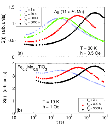
Figure 25: (Color online) $S(t)$ of ZFC relaxation measurements employing different wait times on (a) Ag(11 at% Mn) and (b) Fe_0.5Mn_0.5TiO₃ . The reduced temperature is 0.9 for both samples.

The relaxation rate $S(t)$ determined from isothermal ZFC relaxation experiments is shown in Fig. 25. The sample is quenched (cooled with the maximum cooling rate) from above $T_{\rm g}$ to the measurement temperature $T_{\rm m}$. For both samples $S(t)$ exhibits a peak at $t_{\rm peak}\approx t_{\rm w}$ except for the shortest waiting time $t_{\rm w}=t_{\rm ws}=3$ s (which is the time needed in order to stabilize the temperaturefootstab ). Due to the slow cooling, the system has already been aged for a certain effective time $t_{\rm min}$ when reaching $T_{\rm m}$.rodkenorb2003 From the measurements with $t_{\rm w}=t_{\rm ws}$ we can determine $t_{\rm min}=t_{\rm peak}\approx 20-40$ s. The effective age of the system after a $T$-shift is determined from the time $t_{\rm peak}$ corresponding to the maximum of $S(t)$, as $t_{\rm eff}(t_{\rm w}+t_{\rm min})=(t_{\rm peak})^{1/\mu}$ with $\mu=1$ for the Ag(11 at% Mn) sample at $T\approx 30$ K and $\mu\approx 0.98-0.99$ at $T=17-19$ K for the Fe_0.5Mn_0.5TiO₃ sample.foot_mu We notice that $t_{\rm min}$ can only be determined from isothermal ZFC relaxation measurements, but not from the corresponding ac relaxation measurement.

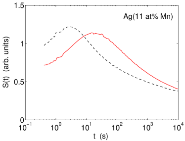
Figure 26: (Color online) $S(t)$ curves obtained for Ag(11 at% Mn) after a rapid cooling ( $v_{\rm cool}\sim 0.05$ K/s) to $T_{\rm m}=30$ K (solid line) and after a rapid cooling to 29 K, where the sample was kept for 3000 s and subsequently heated rapidly ( $v_{\rm heat}\sim 0.5$ K/s) to $T_{\rm m}=30$ K (dashed line).

In Fig. 26, $S(t)$ is shown after a temperature quench ($v_{\rm cool}\sim 0.05$ K/s) to $T_{\rm m}$ and after a $T$-shift to a temperature $T_{\rm i}=29$ K where it is aged for $3000$ s before the temperature is rapidly raised ($v_{\rm heat}\sim 0.5$ K/s) to $T_{\rm m}$. The maximum of the $S(t)$ curve of the $T$-shift experiment appears at $t_{\rm min}\sim 3$ s which is considerably shorter time than $t_{\rm min}\sim 30$ s in the case of quench. The fact that $t_{\rm min}$ is smaller after a positive $T$-shift than after a direct quench implies the system is completely dominated by the strong chaos effect. Namely, $|\Delta T|$ is so large that the intrinsic overlap length $L_{\Delta T}<L_{\rm min}$, where $L_{\rm min}$ is the domain size corresponding to the effective age $t_{\rm min}$. We cannot evaluate the value of $L_{\Delta T}$ itself since it is masked by $L_{\rm min}$ (on heating). $t_{\rm min}$ ($L_{\rm min}$) is smaller on heating than on cooling due to the faster heating than cooling rate and the temperature dependence of the domain growth (c.f. Appendix A). The $L_{\rm min}$ corresponding to $t_{\rm min}$ determined here gives an upper limit for the renormalized overlap length $L_{\rm min}(v_{T},T)$ introduced in Sec. II.6, since the time needed to stabilize the temperature at $T_{\rm m}$ also contributes to $t_{\rm min}$ ($L_{\rm min}$). It is also possible to obtain a random initial configuration with a small $t_{\rm min}$ by using a magnetic field making a “field quench”.noretal87 Throughout this article, we have however only used the ordinary temperature quench to initialize the system.

Appendix C Simulational Details

The Monte Carlo simulations were performed on the 4 dimensional EA Ising model whose critical temperature is $T_{g}/J=2.0$ bercam97 . The simulations were made at the temperatures $T/J=1.2,0.8$ ($T/T_{g}=0.6,0.4$), which are well below the critical temperature so that numerical time/length scales are not strongly affected by critical fluctuations. Systems with $24^{4}$ spins were used, which are large enough to get rid of finite size effects within the numerical time window.yoshuktak2002 The simulations were done using the standard heat-bath Monte Carlo method up to a time scale of $10^{5}$ Monte Carlo Steps (MCS) starting with random spin configurations in order to mimic aging after ideal temperature quenches. The average over at least $32$ different realizations of random bonds were taken. For the measurements of the ZFC susceptibilities $320$ samples were used.

The advantage of the 4 dimensional model compared with the 3 dimensional EA Ising model, which might appear slightly more realistic, is that a rich amount of knowledge about the equilibrium and dynamical properties of the model has been accumulated by independent studies. This includes the critical properties associated with the fixed point at $T_{g}$,bercam97 the $T=0$ glassy fixed point hukushima99 ; hartmann99 and the dynamical length $L_{T}(t)$ obtained in Ref. hukyostak2000, ; yoshuktak2002, . We note that a recent Monte Carlo simulation yoshuktak2002 on the same model confirmed, to a certain extent, certain predictions from the fundamental dynamical scaling ansatz due to the droplet theory bramoo87 ; fishus88eq ; fishus88noneq (including that for the decay of TRM (thermo remanent magnetization) which are all expressed in terms of the dynamical length scale $L_{T}(t)$. It is also worth to mention that in equilibrium Monte Carlo simulations of the model the anticipated signatures of the chaos effect have been observed both in the case of temperature changes hukiba2003 (exchange Monte Carlo method), and bond perturbation.ney98

Unfortunately within the available computational power it is difficult to observe even some weak traces of rejuvenation by temperature changes by the standard heat-bath dynamical Monte Carlo simulations. rieger94 ; komyostak2000A ; picricrit2001 ; berbou2002 ; takhuk2002 ; berbou2003 Within feasible CPU times, one is forced to work at temperatures rather close to $T_{g}$, such as $0.8-0.9T_{g}$. In this temperature range, the dynamics in the numerical time window is strongly affected by critical fluctuations, hukyostak2000 ; yoshuktak2002 ; berbou2002 ; jonyosnor2003 while the experimental time window lies well outside the critical regime jonyosnor2003 (see Fig. 24). Thus we limit ourselves with bond-shift and cycling simulations.

References

- (1) Present address: ISSP, University of Tokyo, Kashiwa-no-ha 5-1-5, Kashiwa, Chiba 277-8581, Japan. E-mail: petra@issp.u-tokyo.ac.jp.
- (2) Present address: ERATO-SSS/JST, Cryogenic Center, University of Tokyo, 2-11-16 Yayoi, Bunkyo-ku, Tokyo 113-0032, Japan.
- (3) V. Cannella and J. A. Mydosh, Phys. Rev. B 6, 4220 (1972).
- (4) S. F. Edwards and P. W. Anderson, J. Phys. F 5, 965 (1975).
- (5) D. Sherrington and S. Kirkpatrick, Phys. Rev. Lett. 35, 1792 (1975).
- (6) J.-P. Bouchaud, L. F. Cugliandolo, J. Kurchan, and M. Mézard, in Spin Glasses and Random Fields, edited by A. P. Young (World Scientific, Singapore, 1997), pp. 161–223.
- (7) J.-P. Bouchaud, in Soft and Fragile Matter, edited by M. E. Cates and M. R. Evans (Institute of Physics Publishing, Bristol and Philadelphia, 2000).
- (8) L. Lundgren, P. Svedlindh, P. Nordblad, and O. Beckman, Phys. Rev. Lett. 51, 911 (1983).
- (9) K. Jonason, E. Vincent, J. Hammann, J.-P. Bouchaud, and P. Nordblad, Phys. Rev. Lett. 81, 3243 (1998).
- (10) T. Jonsson, K. Jonason, P. Jönsson, and P. Nordblad, Phys. Rev. B 59, 8770 (1999).
- (11) P. Doussineau, T. de Lacerda-Arôso, and A. Levelut, Europhys. Lett. 46, 401 (1999).
- (12) L. Bellon, S. Ciliberto, and C. Laroche, Europhys. Lett. 51, 551 (2000).
- (13) H. Mamiya, I. Nakatani, and T. Furubayashi, Phys. Rev. Lett. 82, 4332 (1999).
- (14) P. Jönsson, M. F. Hansen, and P. Nordblad, Phys. Rev. B 61, 1261 (2000).
- (15) R. Mathieu, P. Svedlindh, and P. Nordblad, Europhys. Lett. 52, 441 (2000).
- (16) E. L. Papadopoulou, P. Nordblad, P. Svedlindh, R. Schöneberger, and R. Gross, Phys. Rev. Lett. 82, 173 (1999).
- (17) A. Gardchareon, R. Mathieu, P. E. Jönsson, and P. Nordblad, Phys. Rev. B 67, 052505 (2003).
- (18) A. J. Bray and M. A. Moore, Phys. Rev. Lett. 58, 57 (1987).
- (19) D. S. Fisher and D. A. Huse, Phys. Rev. B 38, 386 (1988).
- (20) D. S. Fisher and D. A. Huse, Phys. Rev. B 38, 373 (1988).
- (21) D. S. Fisher and D. A. Huse, Phys. Rev. B 43, 10728 (1991).
- (22) H. Yoshino, A. Lemaître, and J.-P. Bouchaud, Eur. Phys. J. B 20, 367 (2001).
- (23) F. Scheffler, H. Yoshino, and P. Maass, Phys. Rev. B 68, 060404R (2003).
- (24) H. Yoshino, J. Phys. A 36, 10819 (2003).
- (25) J.-P. Bouchaud, V. Dupuis, J. Hammann, and E. Vincent, Phys. Rev. B 65, 024439 (2001).
- (26) V. Dupuis, E. Vincent, J.-P. Bouchaud, J. Hammann, A. Ito, and H. A. Katori, Phys. Rev. B 64, 174204 (2001).
- (27) L. Berthier and J. P. Bouchaud, Phys. Rev. Lett. 90, 059701 (2003).
- (28) L. Berthier and J. P. Bouchaud, Phys. Rev. B 66, 054404 (2002).
- (29) A. J. Kovacs, Fortschr. Hochpolym. Forsch. 3, 394 (1963).
- (30) P. E. Jönsson, H. Yoshino, and P. Nordblad, Phys. Rev. Lett. 89, 097201 (2002).
- (31) P. E. Jönsson, H. Yoshino, P. Nordblad, H. Aruga Katori, and A. Ito, Phys. Rev. Lett. 88, 257204 (2002).
- (32) P. E. Jönsson, H. Yoshino, and P. Nordblad, Phys. Rev. Lett. 90, 059702 (2003).
- (33) J. R. Banavar and A. J. Bray, Phys. Rev. B 35, 8888 (1987).
- (34) M. Ney-Nifle and H. J. Hilhorst, Physica A 193, 48 (1993).
- (35) T. Aspelmeier, A. J. Bray, and M. A. Moore, Phys. Rev. Lett. 89, 1972021 (2002).
- (36) T. Rizzo and A. Crisanti, Phys. Rev. Lett. 90, 137201 (2003).
- (37) M. Sales and H. Yoshino, Phys. Rev. E 65, 066131 (2002).
- (38) F. Ritort, Phys. Rev. B 50, 6844 (1994).
- (39) M. Ney-Nifle, Phys. Rev. B 57, 492 (1998).
- (40) A. Billoire and E. Marinari, J. Phys. A 33, L265 (2000).
- (41) M. Picco, F. Ricci-Tersenghi, and F. Ritort, Phys. Rev. B 63, 174412 (2001).
- (42) A. Billoire and E. Marinari, Europhys. Lett. 60, 775 (2002).
- (43) H. Takayama and K. Hukushima, J. Phys. Soc. Jpn. 71, 3003 (2002).
- (44) T. Komori, H. Yoshino, and H. Takayama, J. Phys. Soc. Jpn. 69 Suppl. A, 228 (2000).
- (45) L. Berthier and P. C. W. Holdsworth, Europhys. Lett. 58, 35 (2002).
- (46) E. Vincent, J. Hammann, M. Ocio, J.-P. Bouchaud, and L. F. Cugliandolo, in Complex behaviour of glassy systems: proceedings of the XIV Sitges Conference, edited by E. Rubi (Springer, Berlin, 1996).
- (47) G. J. M. Koper and H. J. Hilhorst, J. Phys. (Paris) 49, 429 (1988).
- (48) J. Houdayer and O. C. Martin, Europhys. Lett. 49, 794 (2000).
- (49) F. Krzakala and O. C. Martin, Phys. Rev. Lett. 85, 3013 (2000).
- (50) M. Palassini and A. P. Young, Phys. Rev. Lett. 85, 3017 (2000).
- (51) F. Krzakala.
- (52) Note that in a previous article jonyosnor2003 we have proposed the correction term to be . However term seems more natural since should be an even function of (and ) and analytic at (and ).
- (53) The Mattis model itself does show neither spontaneous bond nor temperature chaos effects. However it is useful to illustrate and examine the ideas of ghost domains because i) the model can be designed to have a desired random spin configuration as its ground state and ii) the dynamics is unambiguously of the domain growth type. The Hamiltonian is formally given as Eq. (1) but with the coupling given as . The backbone spin configuration of the target equilbrium state is unambiguously given by the ground state which is . Here a pinning effect is introduced: is a random number uniformly distributed between and which controls the strength of random pinning which induces domain growth by thermally activated processes. hh85 The dynamics is simulated by a usual single spin flip heat-bath Monte Carlo algorithm. The procedure of the simulation is as the following. First, the Hamiltonian of a ground state is applied a time (initial aging stage). Then, the Hamiltonian of a different ground state is applied an additional time (perturbation stage). Finally, the Hamiltonian is put back to the original one which is applied an additional time (healing stage). The two ground states and are chosen to be completely independent from each other to mimic strong chaos with overlap length . In Fig 3, the lattice has spins. The pinning strength is set and temperature is cycled as with and . The time steps are chosen as (left figures) , , (MCS) and (right figures) , (MCS).
- (54) A. J. Bray and J. G. Kissner, J. Phys. A 25, 31 (1992).
- (55) P. Granberg, L. Lundgren, and P. Nordblad, J. Magn. Magn. Mater. 92, 228 (1990).
- (56) R. L. Leheny and S. R. Nagel, Phys. Rev. B 57, 5154 (1998).
- (57) L. Berthier, V. Viasnoff, O. White, V. Orlyanchik, and F. Krzakala.
- (58) E. Bertin, J.-P. Bouchaud, J.-M. Drouffe, and C. Godreche, J. Phys. A 36, 10701 (2003).
- (59) A. Ito, H. Aruga, E. Torikai, M. Kikuchi, Y. Syono, and H. Takei, Phys. Rev. Lett. 57, 483 (1986).
- (60) A. Ito, E. Torikai, S. Morimoto, H. Aruga, M. Kikuchi, Y. Syono, and H. Takei, J. Phys. Soc. Jpn. 59, 829 (1990).
- (61) J. Magnusson, C. Djurberg, P. Granberg, and P. Nordblad, Rev. Sci. Instrum. 68, 3761 (1997).
- (62) R. Mathieu, P. Jönsson, D. N. H. Nam, and P. Nordblad, Phys. Rev. B 63, 092401 (2001).
- (63) L. W. Bernardi and I. A. Campbell, Phys. Rev. B 56, 5271 (1997).
- (64) H. Rieger, in Annual Review of Computational Physics II, edited by D. Stauffer (World Scientific, ADDRESS, 1995).
- (65) H. Yoshino, K. Hukushima, and H. Takayama, Phys. Rev. B 66, 064431 (2002).
- (66) The non-commercial squid magnetometer used in this study has been designed for a fast temperature stabilization, but a sample with a good heat conductivity is also essential. Under different experimental conditions might be much longer, see e.g. beretal2003, .
- (67) P. Granberg, L. Sandlund, P. Nordblad, P. Svedlindh, and L. Lundgren, Phys. Rev. B 38, 7097 (1988).
- (68) L. Sandlund, P. Svedlindh, P. Granberg, P. Nordblad, and L. Lundgren, J. Appl. Phys. 64, 5616 (1988).
- (69) C. Djurberg, K. Jonason, and P. Nordblad, Eur. Phys. J. B 10, 15 (1999).
- (70) D. Hérisson and M. Ocio, Phys. Rev. Lett. 88, 257202 (2002).
- (71) K. Hukushima, H. Yoshino, and H. Takayama, Prog. Theo. Phys. 138, 568 (2000).
- (72) The values of are obtained for (MCS) by simulating isothermal aging. Some data are shown in Fig. 11(a)). Then is viewed as a function of , and it was fitted to a polynomial of and the resulting smooth fitting function was considerd as the model function of .
- (73) K. Hukushima and Y. Iba.
- (74) Factors that can affect the estimation of are the noise in the ac-signal and the time needed to stabilize the temperature (and the ac-signal) after the cycling.
- (75) M. Sasaki, V. Dupuis, J.-P. Bouchaud, and E. Vincent, Eur. Phys. J. B 29, 469 (2002).
- (76) L. Bellon, S. Ciliberto, and C. Laroche, Eur. Phys. J. B 25, 223 (2002).
- (77) In ac experiments, it is possible to define a frequency dependent freezing temperature from a rather sharp maximum in the in-phase component of the susceptibility. Below this temperature, the longest relaxation time of the system exceeds the observation time () employed and a finite out phase component of the susceptibility appears. approaches for low frequencies, and increases with increasing frequency. In low field dc magnetization measurements, a corresponding maximum is observed in the temperature dependence of the ZFC magnetization. Such an experiment looks at the system on a certain observation time, that by comparison to ac-susceptibility results can be estimated to 10-100 s. By this analogy, we denote this temperature , which was found in our experiments to be equal to 23.6 K for Fe0.5Mn0.5TiO3 and 33.5 K for Ag(11 at% Mn) . In the dc memory experiments, the stop temperatures () were chosen at similar values for both systems.
- (78) R. Mathieu, P. E. Jönsson, P. Nordblad, H. A. Katori, and A. Ito, Phys. Rev. B 65, 012411 (2002).
- (79) In Fig. 23, for the continuous cooling/heating protocol is for simplicity given as . This is based on the observation that in an isothermal aging experiments after temperature quenches down to we find the effective times s (see Fig. 25 and 7). In a memory experiments the cooling/heating rate is lower than the maximum one and we therefore expect to be a bit larger. The exact value of are different on cooling and heating as discussed in Sec. VI.3.
- (80) P. Jönsson, H. Yoshino, H. Mamiya, and H. Takayama.
- (81) M. Lederman, R. Orbach, J. M. Hammann, M. Ocio, and E. Vincent, Phys. Rev. B 44, 7403 (1991).
- (82) F. Lefloch, J. Hammann, M. Ocio, and E. Vincent, Europhys. Lett. 18, 647 (1992).
- (83) L. V. Mikheev, B. Drossel, and M. Kardar, Phys. Rev. Lett. 75, 1170 (1995).
- (84) G. F. Rodriguez, G. G. Kenning, and R. Orbach, Phys. Rev. Lett. 91, 037203 (2003).
- (85) The values of were determined from isothermal ZFC relaxation experiments, where .
- (86) P. Nordblad, P. Svedlindh, P. Granberg, and L. Lundgren, Phys. Rev. B 35, 7150 (1987).
- (87) K. Hukushima, Phys. Rev. E 60, 3606 (1999).
- (88) A. K. Hartmann, Phys. Rev. E 59, 84 (1999).
- (89) H. Rieger, J. Physique (France) I 4, 883 (1994).
- (90) D. A. Huse and C. L. Henley, Phys. Rev. Lett. 54, 2708 (1985).
- (91) F. Bert, V. Dupuis, E. Vincent, J. Hammann, and J.-P. Bouchaud, Phys. Rev. Lett. 92, 167203 (2004).