Mean-field theory of Bose-Fermi mixtures in optical lattices

Abstract

We extend the results of [M. Lewenstein et al., Phys. Rev. Lett. 92, 050401 (2004)] and determine the phase diagram of a mixture of ultracold bosons and polarized fermions placed in an optical lattice using mean field theory. We obtain the analytic form of the phase boundaries separating the composite fermion phases that involve pairing of fermions with one or more bosons, or bosonic holes, from the bosonic superfluid coexisting with Fermi liquid. We compare the results with numerical simulations and discuss their validity and relevance for current experiments. We present a careful discussion of experimental requirements necessary to observe the composite fermions and investigate their properties.

I Introduction

During the last few years, the intensive quest for the Bardeen-Cooper-Schrieffer (BCS) transition RevBCS in ultracold trapped Fermi gases has stimulated the interest in mixtures of fermions and bosons, from now on called Fermi-Bose (FB) mixtures. In these systems, sympathetic cooling techniques can be efficiently used to reach temperatures well down into the regime of quantum degeneracy bfcooling . Recently, the rich physics of FB mixtures has become itself one of the central topics of the physics of ultracold gases. Various phenomena occurring in FB mixtures have been analyzed, including the phase separation between bosons and fermions molmer ; stoof ; pu , the existence of novel types of collective modes stoof ; pu ; capuzzi ; liu , the appearance of effective Fermi-Fermi interactions mediated by the bosons stoof ; pu ; albus ; viverit , the collapse of the Fermi cloud in the presence of attractive interactions between bosons and fermions collapse , or the effects characteristic for the 1D FB mixtures das ; cazalilla .

Recently, the possibility to load ultracold atomic gases in periodic potentials induced by laser standing waves (optical lattices) has attracted considerable attention, motivated partially by the resemblances of these systems to the solid-state ones BECLatt . The remarkable experimental advances on atomic trapping and cooling on one side, and the possibility of manipulation of the interatomic interactions via Feshbach resonances Feshbach on the other, have opened the way towards a fascinating new physics, namely that of strongly correlated ultracold atomic gases in optical lattices. The most important result so far in this brand new research field has been provided by the achievement of the superfluid (SF) to Mott-insulator (MI) transition in bosonic gases jaksch ; bloch .

The experimental success achieved in bosonic gases, has triggered the interest in the physics of BF mixtures in optical lattices, which under appropriate conditions can be well described by the Bose-Fermi Hubbard model (BFH) model eisert ; blatter . A particularly interesting feature resulting from the BFH model is the possibility to produce fermionic composites, formed by the pairing of a fermion and a boson (or a fermion and a bosonic hole) svistunov ; lewen ; kagan ). A Bose-Fermi lattice gas is somewhat similar to the Bose lattice gas of Refs. jaksch ; bloch , although it exhibits a much more complex and richer behavior at low temperatures, as we have recently shown in Ref. lewen .

In Ref. lewen , we have discussed the limit of strong atom-atom interactions (strong coupling regime) at low temperatures, and have predicted the existence of novel quantum phases in lattices that involve the previously mentioned composite fermions, which for attractive (repulsive) interactions between fermions and bosons, are formed by fermion and bosons (bosonic holes). The resulting composite fermions present a remarkably rich phase diagram, and may form, depending on the system parameters, a normal Fermi liquid, a density wave, a superfluid liquid, or an insulator with fermionic domains.

In this paper we significantly extend the analysis of Ref. lewen . In Sec. II we present a description of the model, while in Sec. III we remind the readers the main results of Ref. lewen . In Sec. IV, we determine the phase diagram of the system for arbitrary values of the chemical potential, the Fermi-Bose coupling, and the tunneling (hopping) amplitudes using mean-field theory sachdev . In this sense our results can be considered as a generalization of the seminal analysis of the Bose-Hubbard model by Fisher et al. fisher . We obtain the analytic form of the phase boundaries separating the composite fermion phases from the phase consisting on a bosonic superfluid coexisting with a Fermi liquid. The method we use is a ”traditional” mean field approach, which has a limited domain of applications, but has an advantage of being technically relatively simple. In the case considered in this paper, it can be rigorously confirmed using more sophisticated methods of functional integrals within the quantum field theoretical framework. In Sec. V we compare analytical and numerical results, and discuss their validity and relevance for current experiments. Sec. VI is devoted to a careful discussion of the necessary requirements to observe the composite fermions and investigate their properties in experiments. Finally, we present our conclusions in Sec. VII.

II Bose-Fermi Hubbard model

In this section we present a description of the model in question. Let us consider a sample of ultracold bosonic and (polarized) fermionic atoms trapped in an optical lattice, e.g. ⁷Li-⁶Li or ⁸⁷Rb-⁴⁰K. Due to the periodicity of the lattice potential, the single-atom states form energy bands, as in solid-state systems. If the temperature is low enough and/or the lattice potential wells are sufficiently deep, the atoms can be assumed to occupy only the lowest energy band. Of course, for fermions this is only possible if their number is strictly smaller than the number of lattice sites (filling factor $\rho_{F}\leq 1$). To describe the system under these conditions, we choose a particularly suitable set of single particle states in the lowest energy band, the so-called Wannier states, which are essentially localized at each lattice site. The system is then described by the tight-binding BFH model (for a derivation from a microscopic model, see Ref. eisert ), which is a generalization of the fermionic Hubbard model, extensively studied in condensed matter theory (c.f. Auerbach ):

$$H_{\mathrm{BFH}}=-\sum_{\left\langle ij\right\rangle}(J_{B}b_{i}^{\dagger}b_{j}+J_{F}f_{i}^{\dagger}f_{j}+{\rm h.c.})$$

$$+\sum_{i}\left[\frac{1}{2}Vn_{i}(n_{i}-1)+Un_{i}m_{i}-\mu_{B}n_{i}-\mu_{F}m_{i}\right],$$ (1)

where $b_{i}^{\dagger}$, $b_{j}$, $f_{i}^{\dagger}$, $f_{j}$ are the bosonic and fermionic creation-annihilation operators, $n_{i}=b_{i}^{\dagger}b_{i}$, $m_{i}=f_{i}^{\dagger}f_{i}$, and $\mu_{B}$ and $\mu_{F}$ are the bosonic and fermionic chemical potentials, respectively. The BFH model describes: i) nearest neighbor boson (fermion) hopping, with an associated negative energy, $-J_{B}$ ($-J_{F}$); ii) on-site repulsive boson-boson interactions with an associated energy $V$; iii) on-site boson-fermion interactions with an associated energy $U$, which is positive (negative) for repulsive (attractive) interactions footnote0 .

For large hopping ($\gg U,V$) the low temperature state of the system in 2D and 3D consists of a superfluid of bosons, which condenses in the zero momentum mode, while the fermions form a Fermi liquid. At exact zero temperature, the fermions would presumably form a superfluid state due to the $p$-wave pairing induced by the attractive boson-mediated fermion-fermion interactions viverit . In this letter we are interested in determining the boundary of this hopping-dominated fluid phase. This boundary is of primary experimental relevance, since it sets the possible conditions for the observation of the predicted interaction-dominated quantum phases lewen . In order to determine this boundary, we have to extend the analysis of Ref. lewen to the previously unexplored regime of $J_{B,F}\simeq U,V$. To this aim we formulate the mean-field theory for bosons following the line of Refs. sachdev ; fisher . We shall first consider the case of a small fermionic hopping ($J_{F}\simeq 0$) and a fermionic filling factor $\rho_{F}$ not too close to $1/2$. If $\rho_{F}\simeq 1/2$ the mean-field solution becomes unreliable due to nesting effects and (in 2D) also due to van Hove singularities.

III Composite fermions and strongly correlated quantum phases

Let us first recall the results of Ref. lewen , which concern the limit of interactions much stronger than hopping. Denoting $\alpha=U/V$, one obtains that in the case of vanishing hopping for $\tilde{\mu}-[\tilde{\mu}]+s>\alpha>\tilde{\mu}-[\tilde{\mu}]+s-1$, $s$ holes (or alternatively $-s$ bosons) form with a single fermion the corresponding composite fermion, which is annihilated by $\tilde{f}_{i}=\sqrt{(\tilde{n}-s)!/\tilde{n}!}(b_{i}^{\dagger})^{s}f_{i}$ ( $\sqrt{\tilde{n}!/(\tilde{n}-s)!}(b_{i})^{-s}f_{i}$ ). The inclusion of a small tunneling ($\ll U,V$) as a perturbation leads to an effective Fermi Hubbard Hamiltonian:

$$H_{eff}=-J_{eff}\sum_{\left\langle ij\right\rangle}(\tilde{f}_{i}^{\dagger}\tilde{f}_{j}+{\rm h.c.})+K_{eff}\sum_{\left\langle ij\right\rangle}\tilde{m}_{i}\tilde{m}_{j},$$ (2)

where $\tilde{m}_{i}=\tilde{f}_{i}^{\dagger}\tilde{f}_{i}$, $-J_{eff}$ is the negative energy associated with the nearest neighbor hopping of composite fermions, and $K_{eff}$ is the energy corresponding to the nearest neighbor composite fermion-fermion interactions, which may be repulsive ($>0$) or attractive ($<0$)lukin . This effective model is equivalent to that of spinless interacting fermions (c.f. sachdev ; Shankar ), and, despite its simplicity, has a rich phase diagram.

For $K_{eff}>0$, and $\rho_{F}\ll 1$ (or $1-\rho_{F}\ll 1$), the ground state of $H_{eff}$ corresponds to a Fermi liquid (a metal), and is well described in the Bloch representation. In this limit, as discussed in Ref. lewen , the system is equivalent to a weakly-interacting (even for large $K_{eff}$) Fermi gas of spinless fermions (for $\rho_{F}\ll 1$), or holes (for $1-\rho_{F}\ll 1$). The weakly-interacting picture becomes inadequate for $\rho_{F}\rightarrow 1/2$, and for large $\Delta=K_{eff}/2J_{eff}$, where the effects of the interactions between fermions become important, and one expects the appearance of localized phases. A physical insight on the properties of this regime can be obtained by using Gutzwiller Ansatz (GA) lewen . Defining $\Delta_{crit}=(1+m_{z}^{2})/(1-m_{z}^{2})$, with $m_{z}=2\rho_{F}-1$, one can obtain that for $\Delta<\Delta_{crit}$ the ground state is a Fermi liquid, while for $\Delta>\Delta_{crit}$ it is a density wave with a period of two lattice sites. We expect that the employed GA formalism predicts the phase boundary $\Delta_{crit}$ accurately for $\rho_{F}$ close to $1/2$. For the special case of half filling, $\rho_{F}=1/2$, the ground state is the so-called checkerboard state. For $K_{eff}<0$, and when $|\Delta|\ll 1$, and $\rho_{F}$ is close to zero (one), a very good approach to the ground state is given by a BCS ansatz, in which the composite fermions (holes) of opposite momentum build $p$-wave Cooper pairs. The ground state becomes more complex for arbitrary $\rho_{F}$, and for $\Delta$ approaching $-1$ from above. The system becomes strongly correlated, and the composite fermions in the SF phase may build not only pairs, but also triples, quadruples etc. The situation becomes, however, simpler when $\Delta<-1$, since the composite fermions group into domains, forming what one can call a ”domain” insulator.

IV ”Simple man’s” mean field theory

In order to observe the strongly correlated phases involving the composite fermions it is useful, if not necessary, to know where are their boundaries. Thus, this question has both fundamental and practical character. In this section we will answer this question using perhaps the simplest version of mean field theory. We stress, however, that we have confirmed the results of this section using more sophisticated methods of functional integrals within the quantum field theoretical framework.

In the following we shall consider the case of vanishing temperature, $T\rightarrow 0$, but still $k_{B}T\gg J_{F}$, in such a way that we can safely assume $J_{F}=0$. In order to analyze the relevant intermediate case $J_{B}\simeq U,V$, we employ a mean-field formalism sachdev ; fisher ; stoof2 . We shall analyze only homogeneous phases (it is possible to prove that within the mean-field limit supersolid phases are energetically unfavorable). We introduce the superfluid order parameter $\psi=\langle b_{i}\rangle=\langle b_{i}^{\dagger}\rangle$, for every site $i$. Then, neglecting higher order in the fluctuations, we can substitute $b_{j}^{\dagger}b_{i}=\psi(b_{j}^{\dagger}+b_{i})-\psi^{2}$. In this way, we can model the properties of the complete Hamiltonian $H_{BFH}$ by a sum of single-site Hamiltonians: $H_{MF}=\sum_{i}(H_{0i}-\psi{\cal W}_{i})$, where $H_{0i}=\frac{V}{2}n_{i}(n_{i}-1)+Un_{i}m_{i}-\mu_{F}m_{i}-\mu_{B}n_{i}+2dJ_{B}\psi^{2}$, ${\cal W}_{i}=2dJ_{B}\left(b_{i}+b_{i}^{\dagger}\right)$, and $d$ is the spatial dimension. The mean-field Hamiltonian $H_{MF}$ contains the same on-site terms as those of $H_{BHM}$ and additional terms, which represent the influence of neighboring sites.

As previously discussed, the ground-state of $H_{0i}$ consists of $n(m)=\tilde{n}-sm$ bosons per site, where $m$ is the number of fermions in the site, and $s$ depends on the particular region considered in the phase space. For a given fermionic filling factor $\rho_{F}$, the ground-state presents at every site $m=1$ ($m=0$) fermions with probability $\rho_{F}$ ($1-\rho_{F}$). Therefore the ground-state can be written as:

$$|\phi_{0}\rangle\langle\phi_{0}| = (1-\rho_{F})|n=\tilde{n},m=0\rangle\langle n=\tilde{n},m=0|$$

$$+ \rho_{F}|n=\tilde{n}-s,m=1\rangle\langle n=\tilde{n}-s,m=1|.$$

The zeroth-order energy is of the form $E_{0}+2dJ_{B}\psi^{2}$, where $E_{0}=E_{0}(\tilde{n},0)(1-\rho_{F})+E_{0}(\tilde{n}-s,1)\rho_{F}$, with

$$E_{0}(n,m)=\frac{V}{2}n(n-1)+Unm-\mu_{B}n-\mu_{F}m.$$ (3)

Due to the form of ${\cal W}_{i}$, the lowest order correction introduced by the tunneling occurs at second-order:

$$E_{2} = \psi^{2}\sum_{n}\left\{\frac{|\langle\tilde{n},0|{\cal W}|n,0\rangle|^{2}}{E_{0}(\tilde{n},0)-E_{0}(n,0)}(1-\rho_{F})\right\delimiter 00$$ (4)

$$\left\delimiter 00+\frac{|\langle\tilde{n}-s,1|{\cal W}|n,1\rangle|^{2}}{E_{0}(\tilde{n}-s,1)-E_{0}(n,1)}\rho_{F}\right\}$$

where ${\cal W}=\sum_{i}{\cal W}_{i}$. Following the Landau argument for second-order phase transitions, one can easily write $E=E_{0}+2dJ_{B}r\psi^{2}+{\cal O}(\psi^{4})$, where

$$r = 1+2dJ_{B}\left\{\left(\frac{\tilde{n}+1}{\epsilon(\tilde{n},0)}-\frac{\tilde{n}}{\epsilon(\tilde{n}-1,0)}\right)(1-\rho_{F})\right\delimiter 00$$ (5)

$$\left\delimiter 00+\left(\frac{\tilde{n}-s+1}{\epsilon(\tilde{n}-s,1)}-\frac{\tilde{n}-s}{\epsilon(\tilde{n}-s-1,1)}\right)\rho_{F}\right\}$$

where $\epsilon(n,m)=\mu_{B}-Vn+Um$. If $r>0$ the system minimizes the energy by having $\psi=0$ (normal phase), whereas if $r<0$ a nonzero $\psi$ (superfluid) is energetically favorable. Therefore, the curve $r=0$ describes the boundaries between the phase with a superfluid bosonic gas, and the interaction-dominated phases. In Fig. 1 we have depicted the curves $r=0$ for different values of $\alpha$, and different regions of the $\mu_{B}-J_{B}$ phase space.

V Numerical results

The analytical results of the previous section have been compared with numerical calculations based in the GA approach. Technical details concerning the application of GA for fermions in 2D and 3D are discussed in App. A. The GA method allows a generalization of the analytical results presented above to the case of finite $J_{F}$, and for inhomogeneous phases. In our numerical approach, we first evaluate the Bloch functions for the lowest energy band, and properly combine them to obtain the corresponding Wannier functions, largely localized at each lattice site. Using the Wannier functions it is easy to obtain the coefficients $J_{B}$, $J_{F}$, $U$ and $V$ jaksch . We employ the GA wavefunction: $|\phi\rangle=\prod_{i}\sum_{n_{i}=0}^{N_{max}}\sum_{m_{i}=0}^{1}f_{n_{i},m_{i}}|n_{i},m_{i}>,$ where $n$ denotes the number of bosons and $m$ the number of fermions, and neglect fermionic anticommutation rules between operators at different sites (for a detailed discussion on this point, see App. A). We have checked that the value of the maximal bosonic occupation, $N_{max}$, does not affect the calculations. The coefficients $f_{n,m}$ must satisfy $\sum_{nm}|f_{n,m}|^{2}=1$. In the following, we consider only homogeneous phases, although the calculation can be straightforwardly extended to inhomogeneous phases. Hence, the ground-state can be found by minimizing the energy on a single cell, while using periodic boundary conditions. The energy is minimized by changing the values of the coefficients $f_{n,m}$ using a standard downhill technique. The ground-state is calculated for a given number of bosons and fermions, and for the case $U=0$, $V=0$ and a relative low lattice potential (large $J_{B}$).

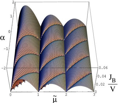
Figure 1: Phase diagram in 2D as a function of $J_{B}/V$, the fermion-boson interactions $\alpha=U/V$, and the bosonic chemical potential $\tilde{\mu}=\mu_{B}/V$, for the case of $J_{F}=0$. The lobes denote the analytical phase boundaries calculated using our mean-field approach. For $\tilde{n}-1<\tilde{\mu}<\tilde{n}$, and $\bar{\mu}-\tilde{n}+s<\alpha<\bar{\mu}-\tilde{n}+s+1$, the number of bosons, $n$, and the number of fermions, $m$, satisfy $n+sm=\tilde{n}$, and composites with one fermion and $s$ bosonic holes ($-s$ bosons) are formed.

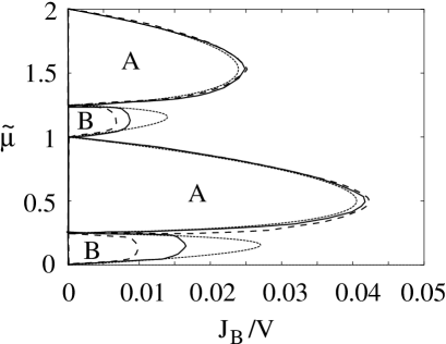
Figure 2: Phase diagram as a function of the hopping $J/V$, and the bosonic chemical potential $\tilde{\mu}=\mu_{B}/V$, for $\alpha=0.25$ and $\rho_{f}=0.25$. Thin solid lines: analytical results for $J_{F}=0$; Bold solid lines: numerical results for $J_{F}=0$; Dashed solid lines : numerical results for $J_{F}=J_{B}$. Phases A are formed by a Mott-Insulator phase for the bosons and a Fermi liquid for the fermions. Phases B are characterized by the formation of fermionic composites with one fermion and one bosonic hole.

Starting from the chosen ground-state, we evolve in the phase space by adiabatically varying the parameters of the system. The time evolution of the $f_{n,m}$ coefficients is obtained by employing the proper minimization $\frac{\partial}{\partial f^{*}_{n,m}}\langle i\hbar\partial_{t}-H\rangle=0$. These equations determine the dynamics of the $f_{n,m}$ coefficients in the phase space, and constitute the basis of what has been called dynamic GA jaksch2 . Since the total number of bosons and fermions is conserved during the time evolution, the chemical potential will be time dependent. This time dependence can be evaluated by calculating two initial ground-states $\psi_{0}(t=0)$ $\psi_{1}(t=0)$ with, respectively, a number of bosons $N_{b}$ and $N_{b}+\delta N$, where $\delta N\ll N_{b}$. We evolve the parallel trajectories while reducing $J_{B}$. The chemical potential can be then approximated as $\mu_{b}(t)\approx\left(\left<\psi_{1}(t)|H(t)|\psi_{1}(t)\right>-\left<\psi_{0}(t)|H(t)|\psi_{0}(t)\right>\right)/\delta N$. By launching various trajectories, we can explore those regions with an incommensurate total number of bosons plus fermions. Consequently, the trajectories do not enter into the regions of the phase diagram in which commensurate phases are expected. Therefore the expected lobular gaps are opened. As shown in Fig. 2, our numerical and analytical results are in good agreement. We must stress that the effects of the fermionic tunneling are not taken into account in the analytic calculations, but they can be easily included in our numerics. In Fig. 2, we also depict a case with finite fermionic tunneling ($J_{B}=J_{F}$). As expected, the lobes of the phases with composite fermions shrink due to the larger mobility of the fermions.

Finally we would like to comment about the validity of the mean-field approach presented in this paper. In general, the mean-field approach is exact at dimension $d=\infty$, and is expected to be reliable for $\tilde{n}\gg 1$, since the relative effects of fluctuations is then small. For the considered cases $\tilde{n}\sim 1$, in a general situation (not at the tips of the lobes) the upper critical dimension is $d_{c}=2$ fisher , and therefore the mean-field approach is reliable. However, at the tips the transition belongs to a different universality class with $d_{c}=3$ fisher , and hence our mean-field approach provides only a qualitative picture.

VI Experimental requirements

Let us finally consider in more detail the necessary requirements to observe the composite fermions and to study their properties. Let us use the notation of Ref. lewen , according to which Roman numbers denote how many particles form a composite, and a bar over the number indicates the composites fermion-bosonic hole(s). In the following discussion we shall assume $J_{F}\simeq J_{B}=J$. We shall consider the regions of the phase diagram which are accessible at easiest:

• Region I : In this region boson-fermion interactions are weak, and we deal with bare fermions. The hopping rate is of order $J$, i.e. relatively big in comparison to the effective interaction energy $K_{eff}$ which is of order $J^{2}/V$.

• Region II : The boson-fermion interactions are attractive, and we deal with composites consisting of one fermion and one boson. Both the hopping rate $J_{eff}$, and the effective interaction energy $K_{eff}$ are of order $J^{2}/V$.

• Region $\bar{\rm II}$ : In this region the boson-fermion interactions are repulsive, and the composites consist of one fermion and one bosonic hole. As in Region II, the hopping rate $J_{eff}$, and the effective interaction energy $K_{eff}$ are of order $J^{2}/V$.

Note, that in the regions III, IV, etc. the effective interactions $K_{eff}$ are of order $J^{2}/V$, but the effective hopping becomes of order $J^{3}/V^{2}$, $J^{4}/V^{3}$, and so on. The larger the composites are obviously the less mobile, and for this reason the observation of their physics is more difficult than for regions I, II or $\bar{\rm II}$.

If we limit ourselves to the Bose-Fermi mixtures in the regime $J<V,U$, there will be then the following temperature regimes:

1. $T>|U|,V$ - This is the high temperature case. The system is a non-degenerated gas of fermions and bosons.

2. $T<|U|,V$ - The bosons enter the MI phase, and the fermions form composites (or remain bare fermions in the region I). Taking into account the fact that the Fermi energy for the effective particles is provided by $J_{eff}$, we have to distinguish two cases:

   1. When $T>J$, the composites constitute a non-degenerated Fermi gas in all considered regions I, II or $\bar{\rm II}$ of the phase diagram.

   2. For $J^{2}/V<T<J$, in the region I a degenerated gas is achieved, since $T<T_{F}$. Since $T>K_{eff}$, however, this gas will behave as a practically ideal gas, since the interaction effects will be masked by the thermal ones. Note, that in the other regions, $T>T_{F}$, because $T_{F}\simeq J_{eff}$. In another words, since the composites in the region II and $\bar{\rm II}$ have a large effective mass, we shall deal in this regime of temperatures with a practically ideal non-degenerated gas of composites.

   3. For $T<J^{2}/V$, in all regions I, II and $\bar{\rm II}$ a degenerated interacting gas of composite fermions is formed, since $T<T_{F}$ and $T<K_{eff}$.

In order to discuss the feasibility of these different temperature regimes, let us introduce the following notation: Let $\sigma=V_{0}/E_{rec}$ be the optical lattice potential $V_{0}$ in units of the photon recoil energy $E_{rec}$, $a_{z}$ - the transversal oscillator length, and $a$ - the atomic scattering length (which, in principle, may be modified using Feshbach-resonance techniques). Approximating the on-site potential by a harmonic oscillator, we obtain that the interaction energy entering the Hubbard model is of the form

$$V/E_{rec}=\sqrt{\frac{\sigma}{2\pi}}\frac{a}{2a_{z}}.$$

According to the results of the present paper, one needs $J/V<0.05$ in order to enter into the strongly correlated phases. That means, in turn, that in order to reach the temperatures in which a degenerated gas of composite Fermions may be observed, i.e. $T<J^{2}/V$, one needs $T<2.5\times 10^{-3}\times\sqrt{\sigma/2\pi}\times(a/2a_{z})T_{rec}\equiv T_{0}$. We recall that for typical experiments, for Lithium atoms $T_{rec}=2.11$ $\mu$K, whereas for Rubidium $T_{rec}=0.17$ $\mu$K. Obviously, lighter atoms (Li) are more favorable.

Of course, the other parameters may be adjusted in various ways. In particular, apart from Feshbach technique, modifications of the transversal traps and lattice height can be used to control the atomic interactions. We have checked that, for instance, such manipulations in the case of ⁶Li-⁷Li mixture, the value of $\alpha=U/V$ may be modified by a factor $4$. This can be easily seen, since

$$\alpha=\frac{2*A*(1+B)}{(1+\sqrt{B*G})(1*B*D)},$$

where $A=a_{BF}/a_{BB}$ is the ratio of scattering lengths, $B=m_{B}/m_{F}$ is the ratio of the masses, $G=V_{0B}/V_{0F}$ is the ratio of optical lattice potentials, and $D=\omega_{zB}/\omega_{zF}$ is the ratio of transverse trapping frequencies for bosons and fermions, respectively.

For instance for ⁶Li-⁷Li mixture $B=7/6$, and taking $G=0.3,D=0.3$, we get $\alpha=2a_{BF}/a_{BB}$, we gain a factor of 2. Assuming some concrete values of the parameters: $a_{BB}=500a_{0}$ (this value demands the employ of a Feshbach resonance), $a_{BF}=30a_{0}$ (with $a_{0}$ being the Bohr radius), we get $\alpha=3/25$. If $\rho_{F}=0.5$ and $\omega_{z}=100$kHz, one obtains then for the region I, $U_{eff}=14.6{\rm nK}$, $U_{BB}=51\mu{\rm K}$, $U_{BF}=6.1\mu{\rm K}$, $J=21.5{\rm nK}$.

The above estimates imply that the previously introduced temperature regimes will be correspond to (1) $T>6$ $\mu$ K, (2) $T<6\ \mu$K, (2b) $T<21$nK (2c) $T<15$nK. From these estimations, and the current experimental state-of-the-art, we conclude that phase (2a), i.e. fermionic composites forming an ideal non-degenerated gas, should be relatively easy to achieve experimentally, since temperatures of the order of $1\mu$K are routinely obtained in current experiments. We would like to stress that such possibility alone could constitute a very interesting experiment by itself. The values to achieve degenerated phases, of the order of $10$nK, are more demanding experimentally, especially due to the difficulties to cool fermions imposed by Pauli-blocking. Nevertheless, this regime of temperatures is definitely not unrealistic, being at the border of what is nowadays achievable. The continuous developments in sympathetic cooling of fermions and bosons allow to foresee that such a regime could be achieved routinely in optical lattices in the nearest future.

VII Conclusions

In conclusion, we have completed the analysis of Ref. lewen by including the tunneling effects within the mean-field theory. This analysis is of crucial experimental importance since sets the conditions for the observability of the interesting phases with composite fermions. We have also developed a numerical method which is in good agreement with our analytics, and additionally provides information for those phases with finite fermionic hopping. Finally, we have analyzed the experimental requirements to observe the predicted effects. In particular, we have discussed different scenarios depending on the system temperature.

We would like to stress that in this paper we have always considered an homogeneous system (no additional external confinement). The analysis of finite temperature effects and inhomogeneities caused by the trap potential mura is interesting in itself, and has been recently the subject of investigations in Ref. jens . Particularly interesting is that a random on-site chemical potential in the presence of Fermi-Bose mixtures can lead to the achievement of various regimes of the physics of quantum fermionic disordered systems spinglass .

Appendix A Validity of simple man’s Gutzwiller ansatz

In this Appendix we discuss some technical details concerning the simple man’s Gutzwiller ansatz for fermions, consisting in writing the variational wave function as a product of on-site Fermi operators, and neglecting the anti-commutation relations between Fermi operators in different sites.

Formally, our variational approach is equivalent to replacing the fermionic annihilation and creation operators $\tilde{f}_{i},\tilde{f}_{i}^{{\dagger}}$ by spin 1/2 operators $\sigma(i),\sigma^{{\dagger}}(i)$. This approach can be justified using the exact Jordan-Wigner transformation in 2D and 3D (fradkin ; eliezer ; huerta , see also tvselik ). In the case of 2D this transformation acquires the form

$$S^{+}(j) = \tilde{f}^{{\dagger}}_{j}\exp\left[i\sum_{k\neq j}\arg(k,j)\tilde{f}_{k}^{\dagger}\tilde{f}_{k}\right],$$ (6)

$$S^{-}(j) = \exp\left[-i\sum_{k\neq j}\arg(k,j)\tilde{f}_{k}^{\dagger}\tilde{f}_{k}\right]\tilde{f}_{j},$$ (7)

$$S_{z}(j) = \tilde{f}^{{\dagger}}_{j}\tilde{f}_{j}-\frac{1}{2},$$ (8)

where $\arg(k,j)$ is the angle between ${\bf k}-{\bf j}$ and an arbitrary space direction on the lattice, which we choose as $x$. The fermionic Hamiltonian of Eq. (2) becomes then

$$H_{eff} = J_{eff}\sum_{\langle i,j\rangle}S^{+}(j)e^{iA(i,j)}S^{-}(i)+h.c.$$ (9)

$$+ K_{eff}\sum_{\langle i,j\rangle}\left(S_{z}(i)+\frac{1}{2}\right)\left(S_{z}(j)+\frac{1}{2}\right),$$

where the “magnetic vector potential”

$$A(i,j)=\sum_{k\neq i,j}[\arg(k,i)-\arg(k,j)](S_{z}(k)+1/2).$$ (10)

The simple man’s Gutzwiller approximation corresponds on this level to i) a variational ansatz for the ground state wave function in the form of product of on-site spin states, and ii) substitution of the “magnetic potential” by its average, which under assumption of mirror reflection symmetry with respect to the lattice axes is zero. Similar approach may be applied in 3D, although in that case the 3D Jordan-Wigner transformation requires an extended Hilbert space and non-Abelian gauge transformations tvselik .

References

- (1) G. V. Shlyapnikov, Proc. XVIII Int. Conf. on Atomic Physics, Eds.: H. R. Sadeghpour, D. E. Pritchard, and E. J. Heller, (World Scientific Publishing, Singapore, 2002).
- (2) A. G. Truscott et al., Science 291, 2570 (2001); F. Schreck et al., Phys. Rev. Lett. 87, 080403 (2001); Z. Hadzibabic et al., Phys. Rev. Lett. 88, 160401 (2002); G. Modugno et al., Phys. Rev. A 68, 011601 (2003); Z. Hadzibabic et al., Phys. Rev. Lett. 91 160401 (2003).;
- (3) K. Mølmer, Phys. Rev. Lett. 80, 1804-1807 (1998).
- (4) M. J. Bijlsma, B. A. Heringa and H. T. C. Stoof, Phys. Rev. A 61, 053601 (2000).
- (5) H. Pu et al., Phys. Rev. Lett. 88, 070408 (2002).
- (6) P. Capuzzi and E. S. Hernández, Phys. Rev. A 64, 043607 (2001).
- (7) X.-J. Liu, and H. Hu, Phys. Rev. A 67, 023613 (2003).
- (8) A. Albus et al., Phys. Rev. A 65, 053607 (2002).
- (9) L. Viverit and S. Giorgini, Phys. Rev. A 66, 063604 (2002).
- (10) G. Modugno et al., Science 297, 2240 (2002).
- (11) K. K. Das, Phys. Rev. Lett. 90, 170403 (2003).
- (12) M. A. Cazalilla and A. F. Ho, cond-mat/0303550.
- (13) B. P. Anderson and M. Kasevich, Science 282, 1686 (1998); O. Mörsch et al., Phys. Rev. Lett. 87, 140402 (2001); W. K. Hensinger et al., Nature 412, 52 (2001); F. S. Cataliotti et al., Science, 293 843 (2001).
- (14) S. Inouye et al., Nature (London) 392, 151 (1998); S. L. Cornish et al., Phys. Rev. Lett. 85, 1795 (2000).
- (15) D. Jaksch et al., Phys. Rev. Lett. 81, 3108 (1998).
- (16) M. Greiner et al., Nature 415, 39 (2002).
- (17) A. Albus, F. Illuminati and J. Eisert, cond-mat/0304223.
- (18) H. P. Büchler and G. Blatter, Phys. Rev. Lett. 91, 130404 (2003).
- (19) A. B. Kuklov and B. V. Svistunov, Phys. Rev. Lett. 90, 100401 (2003).
- (20) M. Lewenstein, L. Santos, M. Baranov and H. Fehrmann, Phys. Rev. Lett. 92, 050401 (2004).
- (21) This phenomenon, related to the appearance of counterflow superfluidity in Ref. svistunov , may occur also in the absence of the optical lattice, M. Yu. Kagan, D. V. Efremov, and A.V. Klaptsov, cond-mat/0209481.
- (22) S. Sachdev, Quantum Phase Transitions, (Cambridge University Press, Cambridge, 1999).
- (23) M. P. A. Fisher, P. B. Weichman, G. Grinstein, and D. S. Fisher, Phys. Rev. B 40, 546-570 (1989)
- (24) For , the single-band model requires smaller than the band gap.
- (25) A. Auerbach, Interacting Electrons and Quantum magnetism, (Springer,New York, 1994).
- (26) L.-M. Duan, E. Demler, and M.D. Lukin, Phys. Rev. Lett. 91, 090402 (2003).
- (27) R. Shankar, Rev. Mod. Phys, 66, 129 (1994).
- (28) D. van Oosten, P. van der Straten, and H. T. C. Stoof, Phys. Rev. A 63, 053601 (2001).
- (29) D. Jaksch et al., Phys. Rev. Lett. 89, 040402 (2002).
- (30) G.G. Batrouni et al., Phys. Rev. Lett. 89, 117203 (2002).
- (31) M. Cramer, J. Eisert, and F. Illuminati, cond-mat/0310705.
- (32) A. Sanpera et al., cond-mat/0402375.
- (33) E. Fradkin, Phys. Rev. Lett. 63, 322 (1989).
- (34) D. Eliezer and G. W. Semenoff, Phys. Lett. B 286, 118 (1992).
- (35) L. Huerta and J. Zanelli, Phys. Rev. Lett. 71, 3622 (1993).
- (36) A. M. Tvselik, “Quantum field theory in condensed matter physics”, Cambridge University Press, 1995.