Permanent address: ]Donetsk Institute for Physics and Technology, 340114 Donetsk, Ukraine

Does a surface spin-flop occur in antiferromagnetically coupled multilayers?
Magnetic states and reorientation transitions in antiferromagnetic superlattices

Abstract

Equilibrium spin configurations and their stability limits have been calculated for models of magnetic superlattices with a finite number of thin ferromagnetic layers coupled antiferromagnetically through (non-magnetic) spacers as Fe/Cr and Co/Ru multilayers. Depending on values of applied magnetic field and unaxial anisotropy, the system assumes collinear (antiferromagnetic, ferromagnetic, various “ferrimagnetic”) phases, or spatially inhomogeneous (symmetric spin-flop phase and asymmetric, canted and twisted, phases) via series of field induced continuous and discontinuous transitions. Contrary to semi-infinite systems a surface phase transition, so-called “surface spin-flop”, does not occur in the models with a finite number of layers. It is shown that “discrete jumps” observed in some Fe/Cr superlattices and interpreted as “surface spin-flop” transition are first-order “volume” transitions between different canted phases. Depending on the system several of these collinear and canted phases can exist as metastable states in broad ranges of the magnetic fields, which may cause severe hysteresis effects. The results explain magnetization processes in recent experiments on antiferromagnetic Fe/Cr superlattices.

Antiferromagnetic coupling in magnetic multilayers mediated by spacer layers and giant magnetoresistance are two related phenomena that have created the basis for applications of antiferromagnetic superlattices as Fe/Cr, Co/Cu, or Co/Ru Grunberg87 . Multilayer stacks with antiferromagnetic interlayer couplings are widely used in spin valves as synthetic antiferromagnets, in various other spinelectronics devices, and they are considered as promising recording media Kim01 . High quality multilayer stacks, such as Co/Ru Ounadjela92 , Fe/Cr(211) Wang94 , or Fe/Cr(001)Temst00 , can be considered as “artificial” nanoscale antiferromagnets. They provide experimental models for the magnetic properties of confined antiferromagnets under influence of surface-effects. Hence, both for applications and from a fundamental point of view, such systems are of great importance and attract much interest in modern nanomagnetism Temst00 ; Steadman02 ; Felcher02 ; Lauter02 ; Nagy02 ; Trallori94 .

In the last years, efforts based on experimental investigations Wang94 ; Temst00 ; Steadman02 ; Felcher02 ; Lauter02 ; Nagy02 , and theoretical studiesWang94 ; Trallori94 to understand ground states and the transitions under magnetic fields in such multilayers resulted in a controversy around the problem of the so-called “surface spin-flop”. This problem can be traced back to Mills’ theory Mills68 which predicted that in uniaxial antiferromagnets spins near the surfaces rotate into the flopped state at a field reduced by a factor of $\sqrt{2}$ compared to the bulk spin-flop field. In an increasing magnetic field such localized surface states spread into the depth of the sample Mills68 . In Ref. Wang94 , the authors claimed to observe these surface states in Fe/Cr superlattices and supported their experimental results by numerical calculations. Subsequent theoretical studies (mostly based on numerical simulations within simplified discretized models Mills68 ) led to conflicting conclusions on the evolution of magnetic states in these systems Trallori94 . Finally, recent experimental investigations obtained different scenarios for reorientational transitions in Fe/Cr Felcher02 ; Lauter02 ; Nagy02 , and Co/Ru Steadman02 multilayer systems.

This study provides a comprehensive analysis within the standard theory of phase transitions to determine all (one-dimensional) spin configurations and their stability limits for models of antiferromagnetic superlattices. Our results explain the diversity of experimentally observed effects in different antiferromagnetic multilayer-systems Wang94 ; Steadman02 ; Temst00 ; Felcher02 ; Lauter02 ; Nagy02 . It is shown that the magnetization processes observed in Wang94 and Felcher02 and interpreted as a manifestation of the “surface spin-flop transitions”, are a succession of first-order phase transitions between asymmetric inhomogeneous phases. Such transitions occur only in a certain range of uniaxial anisotropy. In the major parts of the magnetic field-vs.-uniaxial anisotropy phase diagram the antiferromagnetic phase undergoes discontinuous transitions either into an inhomogeneous spin-flop phase (low anisotropy) or into ferrimagnetic collinear phases (high anisotropy).

The energy of a superlattice with $N$ coupled ferromagnetic layers can be modelled by

$$W = \sum_{i=1}^{N-1}\left[J_{i}\,\mathbf{m}_{i}\cdot\mathbf{m}_{i+1}+\widetilde{J}_{i}\,\left(\mathbf{m}_{i}\cdot\mathbf{m}_{i+1}\right)^{2}\right]-\mathbf{H}\cdot\sum_{i=1}^{N}\mathbf{m}_{i}$$ (1)

$$- \frac{1}{2}\sum_{i=1}^{N}K_{i}\,(\mathbf{m}_{i}\cdot\mathbf{n})^{2}-\sum_{i=1}^{N-1}K^{\prime}_{i}\,(\mathbf{m}_{i}\cdot\mathbf{n})(\mathbf{m}_{i+1}\cdot\mathbf{n})\,,$$

where ${{\mathbf{m}}_{i}}$ are unity vectors along the $i$-th layer magnetization; the first sum includes bilinear ($J_{i}$) and biquadratic ($\widetilde{J}_{i}$) exchange interactions; $K_{i}$ and $K^{\prime}_{i}$ are constants of uniaxial anisotropy and $\mathbf{H}$ is an applied magnetic field. Here, we neglect possible variation of magnetic parameters within the ferromagnetic layers (see PRL01 ). As the magnetic moments of the layers are mesoscopically large, temperature fluctuations do not play a significant role for the magnetic configurations. Thus, we have to find the zero-temperature ground-states described by the energy (1). Temperature dependence enters only indirectly via the phenomenological constants for interlayer exchange and anisotropies. Moreover, we consider the case of antiferromagnetic systems with fully compensated magnetization, i.e systems with even number of ferromagnetic layers. (The noncompensated magnetization in superlattices with odd numbers of layers or with unequal thickness of layers strongly determines their magnetic properties. Such structures are related to ferrimagnetic systems. They could be studied by similar methods as used below, but have to be considered as separate class of systems.)

The type of antiferromagnetic superlattices considered in our analysis are composed of few tens of identical magnetic/nonmagnetic bilayers Ounadjela92 ; Wang94 ; Temst00 ; Felcher02 ; Lauter02 ; Nagy02 ; Steadman02 . To simplify the discussion, we assume that induced interactions in such systems maintain mirror symmetry about the center of the layer stack, i. e. $J_{i}=J_{N-i}$, $K_{i}=K_{N+1-i}$ etc. in the energy (1). Usually demagnetization fields confine the magnetization vectors $\mathbf{m}_{i}$ to the layer plane, and their orientation within this plane can be described by their angles ${\theta_{i}}$ with the easy-axis $\mathbf{n}$. Thus the problem of the magnetic states for the model (1) is reduced to optimization of the function $W(\theta_{1},\theta_{2},...\theta_{N})$. We assume that values of the magnetic parameters are such that the energy (1) yields a collinear antiferromagnetic (AF) phase as ground state in zero field, i.e. $\mathbf{m}_{i}$ are directed along the “easy axis” $\mathbf{n}$ and antiparallel in adjacent layers. Next, we consider the evolution of states with a magnetic field along the easy-axis $\mathbf{n}$.

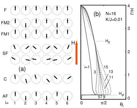
Figure 1: (a) States in antiferromagnetic superlattices (example $N=6$) with increasing field: F ferromagnetic; FM1/2 ferrimagnetic collinear - such phases may be energetically degenerate, but they own different (meta)-stability limits; SF spin-flop states; C asymmetric canted; AF antiferromagnetic). (b) Example of evolution of state with field $H$ for Mills model in low anisotropy case: rotation angles $\theta_{i}$ ($i$ odd) against easy-axis $\bf n$ $||$ field $\bf H$ (for $i$ even $\theta_{i}=-\theta_{N-i+1}$). Phases of type C and FM1/2 may occur only at intermediate and higher anisotropy.

In the case of weak anisotropy ( ${\bar{J}_{i}\equiv J_{i}-2\widetilde{J}_{i}\gg K_{i},K^{\prime}_{i}}$) the applied field stabilizes a spin-flop (SF) phase with symmetric ($\theta_{i}=-\theta_{N-i+1}$) deviations of $\mathbf{m}_{i}$ from the easy -axis (Fig. 1(a)). Contrary to spin-flop phases in bulk antiferromagnets, this SF phase is spatially inhomogeneous. At low fields the solutions for the SF phase are given by a set of linear equations $\bar{J}_{2j-1}(\pi-\theta_{2j-1}+\theta_{2j})=H$, $\theta_{2j}-\theta_{2j+1}=0$ ($j=1,2,...l$, $l=N/4$ for systems with $N=4\,n$ or $l=(N+2)/4$ for $N=4\,n+2$, $n=0,1,\dots$). These solutions describe small deviations of the magnetization vectors, $|\theta_{i}-\pi/2|\ll 1$, from the directions perpendicular to the easy axis (Fig. 1 (a)). Towards top and bottom layer $i=1$ or $N$ in the stack, the deviations increase. For example, for $N=10$ the solutions read $\theta_{5}=\pi/2-H/(2\bar{J}_{5})$, $\theta_{4}=\theta_{5}-\pi$, $\theta_{3}=\theta_{5}-H/\bar{J}_{3}$, $\theta_{2}=\theta_{3}-\pi$, $\theta_{1}=\theta_{3}-H/\bar{J}_{1}$. The properties of these solutions and other particular magnetic configurations of the model (1) arise essentially due to cut exchange bonds at the boundary layers. This is different from surface-induced changes for magnetic states of other nanoscale systems. In ferromagnetic nanostructures, as in nanosized layers of antiferromagnetic materials, noncollinear and/or twisted configurations are caused by particular surface-related anisotropy and exchange contributions due to modified (relativistic) spin-orbit effects near surfaces (as discussed, e.g., in PRL01 ; InFight03 ). The simplified variant of the energy (1) with $J_{i}=J$, $K_{i}=K$, $\widetilde{J}_{i}=K^{\prime}_{i}=0$ embodies this cutting of bonds as the only surface effect and allows to investigate this effect separately from other surface-induced forces. This model, introduced by Mills as a semi-infinite model Mills68 , was later investigated in different cases also for finite systems Wang94 ; Trallori94 . However, in spite of rather sophisticated methods used in these previous studies, the magnetic properties described by this model (called here Mills model) have remained elusive. Transitions and stability lines for the collinear phases can be calculated analytically, but the main body of our results have been obtained by numerical methods. We could investigate in detail systems up to $N=20$ (and some aspects of larger systems) using a combination of methods: (i) search for energy minima using of the order 1000 random starting states for a dense mesh of points in the phase diagram; (ii) an efficient conjugate gradient minimization NR to solve the coupled equations for equilibria $\{\partial W/\partial\theta_{i}=0\}_{i=1\dots N}$; (iii) calculation of stability limits from the evolution of the smallest eigenvalue $e_{0}(H,K)$ of the stability matrix $(\partial^{2}W/\partial\theta_{i}\partial\theta_{j}),i,j=1\dots N$ under changing anisotropy constant $K$ and the applied magnetic field. The basic magnetic configurations are expounded below.

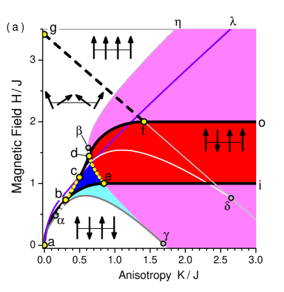
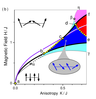
Figure 2: (color) Phase-diagram for Mills model with $N=4$: (a) overview (b) details at low anisotropy ( in this region critical lines have been shifted for clarity). Full black lines are first order transitions between equilibrium states; continuous transitions are dashed and dotted. Equilibrium states: antiferromagnetic below $a-b-e-i$ line (AF); (red) area $o-d-e-i$ collinear “ferrimagnetic” (FM); area $a-b-d-f-g$ symmetric spin-flop phase (SF); (blue) area $b-e-d-c$ noncollinear asymmetric (C); above line $g-f-o$ ferromagnetic phase (FM). Greek letters: critical points at boundaries of metastable states. Metastable states corresponding to FM exist in the region (magenta) right of line $\eta-\beta-d-e-\gamma$ and for C in the two regions $\alpha-b-e-\gamma-\alpha$ and $c-\beta-d-c$ (light blue), respectively. Further stability limits: for SF $a-\alpha-b-c$ and $c-\delta$ (white) $\delta-f-g$; for AF $a-\lambda$ (violet); for FM $g-f-\delta-\zeta$.

(I) Evolution of the inhomogeneous SF phases is given in Fig. 1. At low fields, due to the dominating role of the exchange interactions favouring antiparallel ordering of the magnetizations in adjacent layers, some of the “sublattices” have to rotate against the applied field. At sufficiently strong fields the sense of rotation for these “sublattices” is reversed (Fig. 1(b)). Near saturation, the SF phase has only positive projections of the magnetization on the direction of the magnetic field which decreases towards the center similar to spin configurations described in Ref. Nortermann92 . There is a special field (independent of $N$) where all inner sublattices have the same projection on the field direction ($\theta_{i}=(-1)^{i+1}\,\theta_{0}$, $i=2,3...N-1$) (Fig. 1(b)). The parameters of this “knot” point are determined from the equations $H_{0}/J=(4-k)\cos\theta_{0}$, $\cos(2\theta_{0})=k^{-1}-1/4-\sqrt{1/16+k^{-2}}$, $\theta_{1}+3\,\theta_{0}=\pi$, $k=K/J$.

(II) In the case of strong anisotropy, only collinear (Ising) states minimize the system energy. For Mills model, independently on $N$, there are two discontinuous (“metamagnetic”) transitions: at $H_{1}=J$ to the ferrimagnetic phase with flipped moment at both surfaces (FM) (Fig. 1(a)), and between FM and ferromagnetic (F) phase at $H_{2}=2J$ (Fig. 2).

(III) A specific inhomogeneous asymmetric canted (C) phase (Fig. 1(a)) arises as a transitional low symmetry structure between higher symmetry SF and FM phases. The transition FM $\to$ C is marked by the onset of noncollinearity, i.e. a deviation of $\mathbf{m}_{i}$ from the easy axis, and the transition SF $\to$ C breaks the mirror symmetry.

The calculated phase diagram with $N=4$ in Fig. 2 includes all these phases and elucidates the corresponding magnetization processes for this Mills model. The critical points $b$ and $f$ at $K_{b}\simeq 0.30$ and $K_{f}=\sqrt{2}$ for $N=4$ separate the phase diagram (Fig. 2) into three distinct regions. In the low-anisotropy region ($K<K_{b}$) the first-order transition from AF to the inhomogeneous SF phase occurs at the critical line $a-b$, and a further second-order transition from SF into F phase takes place at the higher field $H_{f}=(2+\sqrt{2})J-K$ (dashed line $g-f$ in Fig. 2). In the high-anisotropy region ($K>K_{f}$) the above mentioned sequence of discontinuous transitions AF $\to$ FM $\to$ F occurs. In this region, different phases can exist as metastable states in extremely broad ranges of magnetic fields leading to severe hysteresis effects. Finally, in the intermediate region $K_{b}<K<K_{f}$ the magnetization processes have a complex character including continuous and discontinuous transitions into the C phase. For $N>4$ the region of the C-phase is subdivided into smaller areas corresponding to canted asymmetric phases separated by first-order critical lines and an area of the reentrant SF phase (Fig. 3). The number of these areas increases with increasing $N$. Here, the evolution of magnetic states occurs as a cascade of discontinuous transitions between different C-phases.

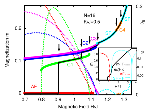
Figure 3: (color) Example of evolution of magnetization (continuous lines and left scales) and lowest eigenvalue of stability matrices $e_{0}$ (dotted, right scales) for Mills model ($N=16$ and $K=0.5$). Black curves: magnetization of equilibrium states, color curves for various “canted” phases C1 $\dots$ C4 and the (reentrant) spin-flop state “SF”. Arrows mark phase transitions. Inset gives full range of field H from antiferromagnetic (AF) to ferromagnetic (F) state (half-logarithmic plot for $e_{0}(H)$) - details are magnified in main figure.

Generally, the function (1) can be considered as the energy of a “multi-sublattice” antiferromagnet with $N$ sublattices each represented by individual ferromagnetic layers. The phase diagram of such an “antiferromagnet” in the space of the magnetic parameters in the model (1) may include a number of new homogeneous and inhomogeneous phases and additional phase transitions. In particular, for nonequal exchange constants there is a cascade of discontinuous transitions between different ferrimagnetic phases, and exchange anisotropy $K^{\prime}_{i}$ may stabilize a twisted phase InFight03 . Moreover, magnetic first-order transitions are generally accompanied by an involved reconstruction of multidomain structures and hysteresis Hubert98 , which will crucially determine the magnetic properties of experimental multilayer systems. However, the basic features of the model (1) are mainly imposed by cut exchange bonds and are revealed from Mills model. The phase diagram in Fig. 2 provides the backbone for the phase diagrams of the whole class of such nanostructures and is representative for their magnetic states.

Our results show that Mills model with finite $N$ owns only well-defined “volume” phases and transitions between them, i.e. phases and transitions affecting the whole layer-stack. The model does not include solutions for surface-confined states, which were assumed to occur at a “surface spin-flop field” $H_{AF}=\sqrt{2JK+K^{2}}$ and to spread into the depth of the sample as the applied field increases up to the “bulk spin-flop field” $H_{B}=\sqrt{4JK+K^{2}}$ Felcher02 ; Mills68 . The critical field $H_{AF}$ determines the stability limit of the “volume” AF phase (violet line $a-\lambda$ in Fig. 2), while the field $H_{B}$ has no physical significance for the finite system. Non-collinear inhomogeneous structures similar to those discussed here as SF phase have been observed in low anisotropic Fe/Cr superlattices Lauter02 . The evolution of multidomain structures accompanying spin-flop transitions was investigated in Nagy02 . Inhomogeneous asymmetric magnetic configurations found in Fe/Cr(211) superlattices with rather large uniaxial anisotropy Wang94 and Felcher02 are similar to C phases discussed in our paper. The magnetization curve Fig. 3 for Mills model with $N=16$ and $K/J=0.5$ amends similar calculations (cf. Fig. 1 (a) in Wang94 ). In addition to the transition from AF into the C-phase, the above described cascade of first-order transitions between different C-phases occurs. A peculiarity of $m(H)$ interpreted as the bulk spin-flop field (in Ref. Wang94 at $H$ = 1.49 kG $\widehat{=}H/J=1.49$) does not correspond to any phase transition.

In conclusion, cut exchange bonds at the boundaries of antiferromagnetic superlattices cause inhomogeneous, noncollinear, or canted magnetic configurations unknown in other types of magnetic nanostructures. Experimental investigations (in particular on superlattices with small number of layers, $N$ = 4 and 6) should provide an interesting play-ground to observe the rich variety of orientational effects predicted in this paper (Fig. 2).

- (1) P. Grünberg, et al., J. Appl. Phys. 61, 3750 (1987); M. N. Baibich, et al., Phys. Rev. Lett. 61, 2472 (1988); I. K. Schuller, S. Kim, and C. Leighton, J. Magn. Magn. Mater. 200, 571 (1999).
- (2) G. J. Strijkers, S. M. Zhou, F. Y. Yang, and C. L. Chien, Phys. Rev. B 62, 13896 (2000); K. Y. Kim, et al., J. Appl. Phys. 89, 7612 (2001). A. Moser, et al., J. Phys. D 35, R157 (2002).
- (3) K. Ounadjela, et al., Phys. Rev. B. 45, 7768 (1992); S. Hamada, K. Himi, T. Okuno, and K. Takanashi, J. Magn. Magn. Mater. 240, 539 (2002).
- (4) R. W. Wang, et al., Phys. Rev. Lett. 72, 920 (1994).
- (5) K. Temst, et al., Physica B 276-278, 684 (2000); V. V. Ustinov, et al., J. Magn. Magn. Mater. 226-230, 1811 (2001).
- (6) P. Steadman, et al., Phys. Rev. Lett. 89, 077201 (2002).
- (7) S. G. E. te Velthuis, J. S. Jiang, S. D. Bader, G.P. Felcher, Phys. Rev. Lett. 89, 127203 (2002).
- (8) V. Lauter-Pasyuk, et al., Phys. Rev. Lett. 89, 167203 (2002); V. Lauter-Pasyuk, et al., J. Magn. Magn. Mater. 258-259, 382 (2003).
- (9) D. L. Nagy, et al., Phys. Rev. Lett. 88, 157202 (2002).
- (10) L. Trallori, et al., Phys. Rev. Lett. 72, 1925 (1994); S. Rakhmanova, D. L. Mills, and E. E. Fullerton, Phys. Rev. B. 57, 476 (1998); N. Papanicolaou, J. Phys.: Condens. Matter 10, L131 (1998); D. L. Mills, J. Magn. Magn. Mater. 198-199, 334 (1999). C. Micheletti, R. B. Griffiths, and J.M. Yeomans, Phys. Rev. B 59, 6239 (1999); M. Momma and T. Horiguchi, Physica A 259, 105 (1998).
- (11) D. L. Mills, Phys. Rev. Lett. 20, 18 (1968); D. L. Mills and W. M. Saslow, Phys. Rev. 171, 488 (1968); F. Keffer and H. Chow, Phys. Rev. Lett. 31, 1061 (1973).
- (12) A. N. Bogdanov and U. K. Rößler, Phys. Rev. Lett. 87, 037203 (2001); A. N. Bogdanov, U. K. Rößler, and K.-H. Müller, J. Magn. Magn. Mater. 238, 155 (2002).
- (13) A. N. Bogdanov, U. K. Rößler, Phys. Rev. B, in press (2003).
- (14) W. H. Press, S. A. Teukolsky, W. T. Vetterling, and B. P. Flannery, Numerical Recipes in C (2nd edition, Cambridge University Press, Cambridge 1992), chap. 10.6.
- (15) F. C. Nörtemann, R. L. Stamps, A. S. Carriço, and R. E. Camley, Phys. Rev. B 46, 10847 (1992); A. L. Dantas and A. S. Carriço, Phys. Rev. B 59, 1223 (1999).
- (16) A. Hubert, R. Schäfer, Magnetic Domains (Springer-Verlag, Berlin, 1998); V. G. Bar’yakhtar, A. N. Bogdanov, and D. A. Yablonskii, Usp. Fiz. Nauk. 156, 47 (1988) [Sov. Phys. Usp. 31, 810 (1988)].