Probing semiclassical analogue gravity in Bose–Einstein condensates
with widely tunable interactions

Abstract

Bose-Einstein condensates (BEC) have recently been the subject of considerable study as possible analogue models of general relativity. In particular it was shown that the propagation of phase perturbations in a BEC can, under certain conditions, closely mimic the dynamics of scalar quantum fields in curved spacetimes. In two previous articles [gr-qc/0110036, gr-qc/0305061] we noted that a varying scattering length in the BEC corresponds to a varying speed of light in the “effective metric”. Recent experiments have indeed achieved a controlled tuning of the scattering length in Rubidium 85. In this article we shall discuss the prospects for the use of this particular experimental effect to test some of the predictions of semiclassical quantum gravity, for instance, particle production in an expanding universe. We stress that these effects are generally much larger than the Hawking radiation expected from causal horizons, and so there are much better chances for their detection in the near future.

I Introduction — Motivation

Semiclassical gravity has played a central role in theoretical physics. Phenomena such as the Hawking effect or cosmological particle production are commonly considered to be crucial first steps on the way to building up a consistent fully-quantum theory of gravity (see for example Birrell-Davies ). However a fundamental limit to these investigations is imposed by the fact that their most basic description is based on linear QFT on a fixed (classical) continuum spacetime. Several theoretical approaches have been developed to overcome this limitation: In a fashion that we can call “top-down”, string models [brane models] have in some special situations developed a high energy description of the Hawking effect Vafa-Strominger , while “bottom-up” approaches, based on Stochastic gravity and the Einstein–Langevin analysis of particle creation by a gravitational field, have in recent years provided further insight Hu1 ; Hu2 .

On the other hand, the physics community has so far lacked any possibility for direct experimental tests of these ideas. Indeed this lack of experimental guidance is a severe hindrance with respect to further developments in semiclassical gravity (or full-fledged quantum gravity for that matter). In particular we have no experimental guidance regarding the manner in which the predictions of curved spacetime quantum field theory are changed once the hypotheses of non-discreteness and/or a non-fluctuating background are relaxed. In this regard the analogue models of gravity developed in recent years can be considered a first attempt to create an arena which can serve as a theoretical, and possibly observational, laboratory to test aspects of these scenarios.

No experimental set up has yet been realized in which the predictions of analogue models can be observationally tested. Nevertheless theoretical analyses of analogue models Unruh ; acoustic have been so far remarkably successful in teaching us how semiclassical gravity phenomena are sensitive to possible quantum gravity effects, such as, for example, modified (Lorentz violating) dispersion relations Parentani . (See for example the trans-Planckian problem in the Hawking effect Unruh and in cosmology Brandenberger .)

What we intend to discuss in this article is a particular class of experiment —that we hope could be realized in the very near future— wherein certain analogue gravity model predictions could be tested. The interest in doing so would not just be that of confirming a now well-established theoretical prediction, but mainly trying to evince deviations from the naive theoretical predictions due to the intrinsic discrete nature of the experimental system and/or to the possible role of non-linearities.

We shall focus our attention on the analogue gravity system established by the propagation of linearized phase perturbations in a Bose-Einstein condensate Garay1 ; Garay2 ; bec-cqg ; abh ; laval ; grf . In particular we shall consider an experiment where a time-varying scattering length is used to simulate the cosmological expansion of the universe, and its associated quantum creation of particles.

It is interesting to note that in reference Hu-Calzetta the authors proposed an explanation of the so called “bosenova” phenomenon bosenova-exp (a controlled instability of the bulk condensate induced by a sign variation of the scattering length) through a particular implementation of a version of analog cosmological particle production. In that approach the entire bulk of the condensate is rendered unstable and suffers catastrophic breakdown. Our current paper takes a complementary approach: Instead of trying to explain an observed phenomenon via analog cosmological particle production, we shall instead consider the most favourable conditions to observe it — preferably without violent disruption of the entire condensate.

The scheme of the paper will be as follows: In the next Section we will review the physics of BECs regarding its analogue gravity features. Section III will be devoted to the discussion of how to simulate a FRW universe within a BEC. There exist two main routes to do this. One considers an explosive expansion of the condensate; the other makes use of the possibility of tuning the strength of the interaction between the different bosons in the condensate. This latter route will be the main concern of this paper.

In Section IV we will first qualitatively describe how the modification of the interaction strength (encoded in the value of the scattering length) yields cosmological particle creation. Next, in Subsection A we will discuss [in the context of current BEC technology] whether there exists a regime in which this particle creation process can actually be reproduced. We will see that there is a limit on the rapidity of change of the background configuration, associated with the need to enforce a “Markov approximation”, in order for the whole construction to make sense. However, this bound still leaves a lot of parameter space available to look for the particle creation effect. Subsection B reviews the cosmological particle creation process, emphasizing the particular features of BEC systems. Then, Subsection C discuss the actual observability of the effect. Finally, we conclude with a short summary and discussion.

II Analogue gravity in Bose–Einstein condensates

Bose-Einstein condensates (BEC) have recently become subject of extensive study as possible analogue models of general relativity Garay1 ; Garay2 ; bec-cqg ; abh ; laval ; grf . In particular it was shown that the propagation of phase perturbations in a BEC can under certain conditions closely mimic the dynamics of quantum fields in curved spacetimes. In previous papers we noted that a varying scattering length in the BEC system corresponds to a varying speed of light in the “effective metric” laval ; grf . Recent experiments have indeed achieved a controlled tuning of the scattering length in Rubidium 85 Rb1 . The effect is powerful enough to lead to large non-perturbative changes in the effective metric. Let us start by very briefly reviewing the derivation of the acoustic metric for a BEC system.

In the dilute gas approximation, one can describe a Bose gas through a quantum field ${\widehat{\Psi}}$ satisfying

$${\rm i}\hbar\;\frac{\partial}{\partial t}{\widehat{\Psi}}=\left(-{\hbar^{2}\over 2m}\nabla^{2}+V_{\rm ext}({\mathbf{x}})+\kappa(a){\widehat{\Psi}}^{\dagger}{\widehat{\Psi}}\right){\widehat{\Psi}}.$$ (1)

Here $\kappa$ parameterizes the strength of the interactions between the different bosons in the gas. It can be re-expressed in terms of the scattering length as

$$\kappa(a)={4\pi a\hbar^{2}\over m}.$$ (2)

As usual, the quantum field can be separated into a macroscopic (classical) condensate and a fluctuation: ${\widehat{\Psi}}=\psi+{\widehat{\varphi}}$, with $\langle{\widehat{\Psi}}\rangle=\psi$. Then, by adopting the self-consistent mean field approximation Griffin

$${\widehat{\varphi}}^{\dagger}{\widehat{\varphi}}{\widehat{\varphi}}\simeq 2\langle{\widehat{\varphi}}^{\dagger}{\widehat{\varphi}}\rangle{\widehat{\varphi}}+\langle{\widehat{\varphi}}{\widehat{\varphi}}\rangle{\widehat{\varphi}}^{\dagger},$$ (3)

one can arrive at the set of coupled equations:

$${\rm i}\hbar\;\frac{\partial}{\partial t}\psi(t,{\mathbf{x}})=\left(-{\hbar^{2}\over 2m}\nabla^{2}+V_{\rm ext}({\mathbf{x}})+\kappa\;n_{c}\right)\psi(t,{\mathbf{x}})+\kappa\left(2\tilde{n}\psi(t,{\mathbf{x}})+\tilde{m}\psi^{*}(t,{\mathbf{x}})\right);$$ (4)

$${\rm i}\hbar\;\frac{\partial}{\partial t}{\widehat{\varphi}}=\left(-{\hbar^{2}\over 2m}\nabla^{2}+V_{\rm ext}({\mathbf{x}})+\kappa\;2n_{T}\right){\widehat{\varphi}}+\kappa\;m_{T}\;{\widehat{\varphi}}^{\dagger}.$$ (5)

Here

$$n_{c}\equiv\left|\psi(t,{\mathbf{x}})\right|^{2};\hskip 56.9055ptm_{c}\equiv\psi^{2}(t,{\mathbf{x}});$$ (6)

$$\tilde{n}\equiv\langle{\widehat{\varphi}}^{\dagger}{\widehat{\varphi}}\rangle;\hskip 76.82234pt\tilde{m}\equiv\langle{\widehat{\varphi}}{\widehat{\varphi}}\rangle;$$ (7)

$$n_{T}=n_{c}+\tilde{n};\hskip 68.28644ptm_{T}=m_{c}+\tilde{m}.$$ (8)

The equation for the classical wave function of the condensate is closed only when the back-reaction effect due to the fluctuations are neglected. (This back-reaction is hiding in the parameters $\tilde{m}$ and $\tilde{n}$.) This is the approximation contemplated by the Gross-Pitaevskii equation. In general one will have to solve both equations simultaneously.

Adopting the Madelung representation for the wave function of the condensate

$$\psi(t,{\mathbf{x}})=\sqrt{n_{c}(t,{\mathbf{x}})}\;\exp[-{\rm i}\theta(t,{\mathbf{x}})/\hbar],$$ (9)

and defining an irrotational “velocity field” by ${\mathbf{v}}\equiv{\mbox{\boldmath$\nabla$}\theta}/{m}$, the Gross-Pitaevskii equation can be rewritten as a continuity equation plus an Euler equation:

$$\frac{\partial}{\partial t}n_{c}+\mbox{\boldmath$\nabla$}\cdot({n_{c}{\mathbf{v}}})=0,$$ (10)

$$m\frac{\partial}{\partial t}{\mathbf{v}}+\mbox{\boldmath$\nabla$}\left(\frac{mv^{2}}{2}+V_{ext}(t,{\mathbf{x}})+\kappa n_{c}-\frac{\hbar^{2}}{2m}\frac{\nabla^{2}\sqrt{n_{c}}}{\sqrt{n_{c}}}\right)=0.$$ (11)

These equations are completely equivalent to those of an irrotational and inviscid fluid apart from the existence of the so-called quantum potential $V_{\rm quantum}=-\hbar^{2}\nabla^{2}\sqrt{n_{c}}/(2m\sqrt{n_{c}})$, which has the dimensions of an energy. Note that

$$n_{c}\;\nabla_{i}V_{\rm quantum}\equiv n_{c}\;\nabla_{i}\left[-{\hbar^{2}\over 2m}{\nabla^{2}\sqrt{n_{c}}\over\sqrt{n_{c}}}\right]=\nabla_{j}\left[-{\hbar^{2}\over 4m}\;n_{c}\;\nabla_{i}\nabla_{j}\ln n_{c}\right],$$ (12)

which justifies the introduction of the so-called quantum stress tensor

$$\sigma_{ij}^{\rm quantum}=-{\hbar^{2}\over 4m}\;n_{c}\;\nabla_{i}\nabla_{j}\ln n_{c}.$$ (13)

This tensor has the dimensions of pressure, and may be viewed as an intrinsically quantum anisotropic pressure contributing to the Euler equation. If we write the mass density of the Madelung fluid as $\rho=m\;n_{c}$, and use the fact that the flow is irrotational then the Euler equation takes the form

$$\rho\left[\frac{\partial}{\partial t}{\mathbf{v}}+({\mathbf{v}}\cdot\mbox{\boldmath$\nabla$}){\mathbf{v}}\right]+\rho\;\mbox{\boldmath$\nabla$}\left[\frac{V_{ext}(t,{\mathbf{x}})}{m}\right]+\mbox{\boldmath$\nabla$}\left[{\kappa\rho^{2}\over 2m^{2}}\right]+\mbox{\boldmath$\nabla$}\cdot\sigma^{\rm quantum}=0.$$ (14)

Note that the term $V_{ext}/m$ has the dimensions of specific enthalpy, while $\kappa\rho^{2}/(2m)$ represents a bulk pressure. When the gradients in the density of the condensate are small one can neglect the quantum stress term leading to the standard hydrodynamic approximation. Because the flow is irrotational, the Euler equation is often more conveniently written in Hamilton–Jacobi form:

$$m\frac{\partial}{\partial t}\theta+\left(\frac{(\mbox{\boldmath$\nabla$}\theta)^{2}}{2m}+V_{ext}(t,{\mathbf{x}})+\kappa n_{c}-\frac{\hbar^{2}}{2m}\frac{\nabla^{2}\sqrt{n_{c}}}{\sqrt{n_{c}}}\right)=0.$$ (15)

Apart from the wave function of the condensate itself, we also have to account for the [typically small] quantum perturbations of the system (5). These quantum perturbations can be described in several different ways, here we are interested in the “quantum acoustic representation”

$$\widehat{\varphi}(t,{\mathbf{x}})= e^{-{\rm i}\theta/\hbar}\left({1\over 2\sqrt{n_{c}}}\;\widehat{n}_{1}-{\rm i}{\sqrt{n_{c}}\over\hbar}\;\widehat{\theta}_{1}\right),$$ (16)

where $\widehat{n}_{1},\widehat{\theta}_{1}$ are real quantum fields. By using this representation equation (5) can be rewritten as

$$\partial_{t}\widehat{n}_{1}+{1\over m}\mbox{\boldmath$\nabla$}\cdot\left(\widehat{n}_{1}\;\mbox{\boldmath$\nabla$}\theta+n_{c}\;\mbox{\boldmath$\nabla$}\widehat{\theta}_{1}\right)=0,$$ (17)

$$\partial_{t}\widehat{\theta}_{1}+{1\over m}\mbox{\boldmath$\nabla$}\theta\cdot\mbox{\boldmath$\nabla$}\widehat{\theta}_{1}+\kappa(a)\;n_{1}-{\hbar^{2}\over 2m}\;D_{2}\widehat{n}_{1}=0.$$ (18)

Here $D_{2}$ represents a second-order differential operator obtained from linearizing the quantum potential. Explicitly:

$$D_{2}\,\widehat{n}_{1} \equiv -{1\over 2}n_{c}^{-3/2}\;[\nabla^{2}(n_{c}^{+1/2})]\;\widehat{n}_{1}+{1\over 2}n_{c}^{-1/2}\;\nabla^{2}(n_{c}^{-1/2}\;\widehat{n}_{1}).$$ (19)

The equations we have just written can be obtained easily by linearizing the Gross-Pitaevskii equation around a classical solution: $n_{c}\rightarrow n_{c}+\widehat{n}_{1}$, $\phi\rightarrow\phi+\widehat{\phi}_{1}$. It is important to realize that in those equations the back-reaction of the quantum fluctuations on the background solution has been assumed negligible.

We also see in those equations, (17) and (18), that time variations of $V_{ext}$ and time variations of the scattering length $a$ appear to act in very different ways. Whereas the external potential only influences the background equation (15) [and hence the acoustic metric in the analog description], the scattering length directly influences both the perturbation and background equations.

From the previous equations for the linearized perturbations it is possible to derive a wave equation for $\widehat{\theta}_{1}$ (or alternatively, for $\widehat{n}_{1}$). All we need is to substitute in equation (17) the $\widehat{n}_{1}$ obtained from equation (18). This leads to a PDE that is second-order in time derivatives but infinite order in space derivatives — to simplify things we can construct the symmetric $4\times 4$ matrix

$$f^{\mu\nu}(t,{\mathbf{x}})\equiv\left[\matrix{f^{00}&\vdots&f^{0j}\cr\cdots\cdots&\cdot&\cdots\cdots\cdots\cdots\cr f^{i0}&\vdots&f^{ij}\cr}\right].$$ (20)

(Greek indices run from $0$–$3$, while Roman indices run from $1$–$3$.) Then, introducing $(3+1)$–dimensional space-time coordinates — $x^{\mu}\equiv(t;x^{i})$ — the wave equation for $\theta_{1}$ is easily rewritten as

$$\partial_{\mu}(f^{\mu\nu}\;\partial_{\nu}\widehat{\theta}_{1})=0.$$ (21)

Where the $f^{\mu\nu}$ are differential operators acting on space only:

$$f^{00} = -\left[\kappa(a)-{\hbar^{2}\over 2m}\;D_{2}\right]^{-1}$$ (22)

$$f^{0j} = -\left[\kappa(a)-{\hbar^{2}\over 2m}\;D_{2}\right]^{-1}\;{\nabla^{j}\theta_{0}\over m}$$ (23)

$$f^{i0} = -{\nabla^{i}\theta_{0}\over m}\;\left[\kappa(a)-{\hbar^{2}\over 2m}\;D_{2}\right]^{-1}$$ (24)

$$f^{ij} = {n_{c}\;\delta^{ij}\over m}-{\nabla^{i}\theta_{0}\over m}\;\left[\kappa(a)-{\hbar^{2}\over 2m}\;D_{2}\right]^{-1}\;{\nabla^{j}\theta_{0}\over m}.$$ (25)

Now, if we make an spectral decomposition of the field $\widehat{\theta}_{1}$ we can see that for wavelengths larger than $\hbar/mc_{s}$ (this corresponds to the “healing length”, as we will explain below), the terms coming from the linearization of the quantum potential (the $D_{2}$) can be neglected in the previous expressions, in which case the $f^{\mu\nu}$ can be approximated by numbers, instead of differential operators. (This is the heart of the acoustic approximation.) Then, by identifying

$$\sqrt{-g}\;g^{\mu\nu}=f^{\mu\nu},$$ (26)

the equation for the field $\widehat{\theta}_{1}$ becomes that of a (massless minimally coupled) quantum scalar field over a curved background

$$\Delta\theta_{1}\equiv\frac{1}{\sqrt{-g}}\;\partial_{\mu}\left(\sqrt{-g}\;g^{\mu\nu}\;\partial_{\nu}\right)\widehat{\theta}_{1}=0,$$ (27)

with an effective metric of the form

$$g_{\mu\nu}(t,{\mathbf{x}})\equiv{n_{c}\over m\;c_{s}(a,n_{c})}\left[\matrix{-(c_{s}(a,n_{c})^{2}-v^{2})&\vdots&-v_{j}\cr\cdots\cdots\cdots\cdots&\cdot&\cdots\cdots\cr-v_{i}&\vdots&\delta_{ij}\cr}\right].$$ (28)

Here the magnitude $c_{s}(n_{c},a)$ represents the speed of the phonons in the medium:

$$c_{s}(a,n_{c})^{2}={\kappa(a)\;n_{c}\over m}.$$ (29)

III Analog models for cosmological spacetimes

To find analog models for cosmological spacetimes we will consider a generalized GP equation where the external potential and the coupling constant can both change with time

$${\rm i}\hbar\;\frac{\partial}{\partial t}\psi(t,{\mathbf{x}})=\left(-{\hbar^{2}\over 2m}\nabla^{2}+V_{\rm ext}(t,{\mathbf{x}})+\kappa(t)\;\left|\psi(t,{\mathbf{x}})\right|^{2}\right)\psi(t,{\mathbf{x}}).$$ (30)

The technical steps in the calculation change in a straightforward manner and lead to a simple time-dependent acoustic metric

$$ds^{2}={n_{c}\over m\;c_{s}}\left[-(c_{s}^{2}-v^{2})\,dt^{2}-2\vec{v}\cdot d\vec{x}\,dt+d\vec{x}^{2}\right]$$ (31)

it is this time-dependent effective metric that we now wish to use for simulating a cosmological spacetime and, subsequently probing cosmological particle production.

III.1 Cosmological analog by explosion

Starting from the geometry (31) there are different ways in which one can reproduce a cosmologically expanding geometry. Following grf ; Fischer ; Kagan-Castin ; Kagan one can take a radial profile for the velocity $\vec{v}=(\dot{b}/b)\vec{r}$, with $b$ a scale factor depending only on $t$, and define a new radial coordinate as $r_{b}=r/b$. In these new coordinates, the metric will be expressed as

$$ds^{2}={n_{c}\over m\;c_{s}}\left[-c_{s}^{2}dt^{2}+b^{2}(dr_{b}^{2}+r_{b}^{2}d\Omega_{2}^{2})\right].$$ (32)

Now, one solution for the BEC wave function that reproduces a FRW universe is this: Introducing a Hubble-like parameter,

$$H_{b}(t)={\dot{b}(t)\over b(t)},$$ (33)

the equation of continuity can be written as

$$\dot{n}_{c}+3H_{b}(t)\;n_{c}=0;\qquad\Rightarrow\qquad n_{c}(t)={n_{0}\over b^{3}(t)},$$ (34)

with $n_{0}=$constant. Then, the solution for $\theta$ can be obtained from (15)

$$\theta={\dot{b}\over 2b}mr^{2}+\int_{0}^{t}dt\;{\kappa n_{0}\over b^{3}(t)},$$ (35)

and it requires an external potential of the form

$$V_{\rm ext}(t,r)=-\left({\ddot{b}\over 2b}+{\dot{b}^{2}\over b^{2}}\right)mr^{2}.$$ (36)

One could certainly construct such a potential in a “sufficiently large” region around $r=0$; this would correspond to a “sufficiently large” part of a homogeneous and flat FRW universe. Outside this region, the potential will have in practice some confining walls. The final effective metric can be written as

$$ds^{2}=-T^{2}(t)\;dt^{2}+a_{s}^{2}(t)\;(dr_{b}^{2}+r_{b}^{2}d\Omega_{2}^{2}),$$ (37)

with

$$a_{s}(t)\equiv\left({n_{0}\over m\;\kappa}\;b\right)^{1/4},\qquad\hbox{and}\qquad T(t)\equiv{n_{0}^{3}\over m^{3}\;\kappa^{2}}{1\over a_{s}^{9}(t)}.$$ (38)

So finally we end up with a FRW universe whose proper Friedmann time, $\tau$, is related to the laboratory time, $t$, by $\tau=\int T(t)dt$.

Although this explosion route seems promising, one should note that this analog models has substantial drawbacks. In particular it is easy to see from equation (35) that one would get for the condensate a linearly rising velocity field ${\mathbf{v}}\equiv{\mbox{\boldmath$\nabla$}\theta}/{m}\propto r$. Hence this particular realization of a FRW effective geometry is guaranteed to possess an apparent horizon, a spherical surface in which the speed of the fluid surpasses the speed of sound. From a dynamical point of view, this might introduce many practical problems not intrinsically inherent to the type of geometries we are trying to reproduce. Because of this, we view the use of an exploding medium as not being the preferred route for building an analogue for an expanding FRW universe. (For an alternate view, where the explosion route is the primary focus of attention, see Fischer .)

III.2 Cosmological analog by varying speed of sound

Another way to reproduce cosmologically expanding configurations in, we think, a cleaner fashion is by taking advantage of the possibility to change the value of the scattering length offered by some BECs Rb1 . Let us note that in reference Kagan , the authors already used the existence of time dependence on the scattering length, in combination with a time dependent external potential, to create explosive configuration of the type described in previous subsection. Here, we are going to use this variability with a different strategy.

Let us again start from (31) but now with $v=0$ at all times:

$$ds^{2}=-{n_{c}c_{s}\over m}\;dt^{2}+{n_{c}\over m\;c_{s}}\;d\vec{x}^{2}.$$ (39)

Then, it is not difficult to envisage a situation in which $n_{c}$ is constant in a “sufficiently large” region (think of a “sufficiently large” close-to-hard-walled box). Then, the continuity equation is directly satisfied and the Hamilton–Jacobi equation tells us that with a fixed external potential the phase function $\theta$ will depend only on $t$ adapting itself to the changes of $\kappa(t)$. Changing the scattering length with time directly causes changes in the value of the propagation speed $c_{s}$. (That temporal changes in the velocity of sound can be interpreted as a cosmological expansion without invoking any sort of velocity in the medium has already been suggested in Volovik in the context of superfluid Helium.) We now define $\tau=\int[n_{c}c_{s}(t)/m]^{1/2}dt$ and write

$$ds^{2}=-d\tau^{2}+a_{s}^{2}(\tau)\,d\vec{x}^{2},$$ (40)

where

$$a_{s}(\tau)=\left({n_{c}\over m\;c_{s}(\tau)}\right)^{1/2}=\left({n_{c}\over m\;\kappa(a)}\right)^{1/4}=\left({n_{c}\over 4\pi\hbar^{2}}\right)^{1/4}{1\over a^{1/4}}\equiv{A\over a^{1/4}}.$$ (41)

In this model an expansion corresponds to a decrease of the scattering length and vice versa. The Hubble function for this spacetime is

$$H={a_{s}^{\prime}\over a_{s}}=-{1\over 2}{c_{s}^{\prime}\over c_{s}}=-{1\over 2}\left({m\over n_{c}}\right)^{1/2}\;{\dot{c}_{s}\over c_{s}^{3/2}}.$$ (42)

(The prime represents derivative with respect Friedmann time, the dot derivative with respect laboratory time). This is the model we will consider in the following discussion.

IV Analog cosmological particle creation

Let us now present a qualitative explanation of how is that we can closely simulate cosmological particle creation within this model. We can start with a condensate in a stationary state described, in a sufficiently large volume, by a constant background density $n_{c}$ and a phase function linear in time, $\theta=E_{0}\,t$. This is a solution of the GP equation. For this, one needs to have a potential that reproduces a large enough close-to-hard-walled box and that satisfies the condition $E_{0}=-V_{\rm ext}-\kappa n_{c}$. Apart from this classical background, there will be some quantum fluctuations over it. At temperatures much below the critical temperature these quantum fluctuations are very small and can be described by the Bogoliubov equations. (These quantum fluctuations are present even at zero temperature owing to the so-called quantum depletion phenomenon, see for example Castin .) Let us consider that these quantum fluctuations are in their vacuum state. If one now decreases the value of the scattering length in a sufficiently slow manner (this issue will be discussed bellow), all the individual bosons (this is only an approximate concept in an interacting theory) will be affected in the same way. This means that the value of the background magnitudes —these are the coherent magnitudes— will be slowly modified. The GP equation tells you that the density function $n_{c}$ will be kept fixed while the phase function will develop a non-trivial dependence with time. At the same time the value of the speed of sound will decrease.

Now, apart from the background configuration, what happens with the additional quantum fluctuations? The equation satisfied by the quantum fluctuations is, in the acoustic approximation (that is, for long wavelengths) that of a massless minimally coupled scalar field over an expanding background and therefore, it will yield cosmological pair production of particles.

An interesting point to notice is that varying the external potential —by this we mean changing with time the value of the external potential, $V_{\rm ext}(t)$, in the central homogeneous region— changes the background configuration in the same manner as varying the scattering length does. However, as the speed of sound does not depend on the external potential, its variations will not lead to cosmological particle creation.

Now, what can we say about the observability of the particle production process? The standard technique to “see” phonons is tomographic imaging. One opens the trap and looks at the expansion of the condensate. Phonons correspond to distributions for the momentum of the atoms in the trap and different momenta correspond to different travel distances of the atoms after you switch of the trap. Taking snapshots of this evolution shows the density contrasts and then the original momentum distribution.

If the wave function $\widehat{\Psi}$ is split into the condensate wave function $\psi$ plus quantum excitations $\widehat{\varphi}$ (in this situation, we mean atoms) then, the density you observe is

$$\langle\widehat{\Psi}^{\dagger}\widehat{\Psi}\rangle=|\psi|^{2}+\langle\widehat{\varphi}^{\dagger}\widehat{\varphi}\rangle,$$ (43)

as $\langle\widehat{\varphi}^{\dagger}\rangle=\langle\widehat{\varphi}\rangle=0$. Therefore, the observability of the effect will depend on the value of the ratio

$${\langle\widehat{\varphi}^{\dagger}\widehat{\varphi}\rangle\over|\psi|^{2}}={1\over n_{c}}\langle\widehat{\varphi}^{\dagger}\widehat{\varphi}\rangle$$ (44)

or more simply on the spatially integrated ratio

$$C\equiv{1\over N_{c}}\int dx^{3}\langle\widehat{\varphi}^{\dagger}\widehat{\varphi}\rangle.$$ (45)

If this quantity is of order unity (say 1/2 or 1/10) then phonons can probably be “seen”; if it is 1/100 then seeing phonons is technologically difficult. If the particle production process was so strong that the calculation of $C$ resulted on values close to unity or higher, this would indicate that the Bogoliubov mean field approximation would have been violated, and the BEC itself disrupted.

Let us now perform some explicit calculations of the particle production expected in realistic situations with present-day BECs in which the scattering length $a$ is changed in time from some initial value to a different final value. We first have to know how quickly we can drive these temporal changes while still ensuring that the different approximations involved in the analysis remain valid.

IV.1 Varying $a$, validity of the GP equation

The previous analysis shows that in order to consider particle creation driven by a time-varying scattering length we must be sure to work in a regime where the background is “instantaneously” reacting to the changes in $a$. Moreover the very derivation of the effective metric description is based on the GP equation which we then want to make sure holds at each instant of time.

So we must first determine the upper bound on the rapidity of the change in the scattering length $a$ which still permits the GP equation to hold. This will also give an upper bound for the frequencies of the quasi-particles that might be created (if $\tau$ is the shortest timescale over which we can drive the system then $\nu\approx 1/\tau$ is the largest frequency of the quasi-particle we can create). The validity of the GP in describing the Bose-Einstein condensate is related to the validity of several crucial assumptions which permit us to perform certain approximations on the fundamental multi-particle Hamiltonian description. The relevant approximations are generally stated to be the “mean-field” approximation and the dilute gas approximation. It is nevertheless important to note that in a dynamical situation a third approximation, which we can call “Markovian” approximation, is implicitly assumed.

Let us review the meaning and implications of these approximations: The mean field approximation is based on the assumption that most of the atoms are in the condensate phase and that the influence of the non condensed fraction can be neglected. This implies that significant creation of quasi-particles with excessive energies can be dangerous. In particular from the Bogoliubov dispersion relation broken

$$\omega=\sqrt{c_{s}^{2}k^{2}+\left({\hbar\over 2m}\;k^{2}\right)^{2}},$$ (46)

we can deduce that excitation of quasi-particles with wavelengths comparable to the healing length would led to free particle states (for $k>2\pi/\xi$; $\xi=\hbar/(m\;c_{s})$; $\omega\approx\hbar^{2}k^{2}/(2m)$). This argument seems to imply that one should require the typical timescale for the change in $a$ to be no shorter than the healing time. (Which is the analogue in this situation of the Planck time in quantum gravity.)

The dilute gas approximation is instead related to the way the interaction potential is simplified in the GP equation. This approximation is valid if $n|a|^{3}\ll 1$, so we shall have to keep the amplitude of the changes in $na^{3}$ small in order to satisfy this bound. We wish to emphasise that the dilute gas approximation does not appear to be a crucial approximation for the analog gravity picture to hold. As long as the interaction term $\kappa|\psi(t,{\mathbf{x}})|^{2}$ can be generalized to be some higher order (but still local) term $\pi(|\psi|)$ an analog gravity description is not precluded (see, for example bec-cqg ).

Finally the Markovian approximation is related to the fact that in dynamical situations the two-body time-dependent scattering matrix can have a complicated form due to the “memory” of the system (see e.g. section IV-A of the paper by Köhler and Burnett Kohler-Burnett ). Basically in these situations the system is described by a GP-like equation where the interaction term includes a “delay term” described by an integration over different times. The necessary assumption in order to have a Markovian description of the dynamics (which together with the two previous approximations leads to the GP equation) is then that the timescales on which external parameters are changing are longer that the two-body collisional duration. That is, longer than the timescale over which a single interaction happens. (Reduced to the bare bones, we are asking that the scattering length does not change significantly during the period when a pair of atoms are interacting.)

We can estimate the two-body collisional time by a simple calculation. All we need is the typical size of the region of strong interaction of two atoms in the condensate and the typical speed with which they move. The first quantity can be assumed to be of the order of the Van der Waals scale length: the inter-atomic potential $V(r)$ is characterized by a short-range region of strong chemical bonding and a long-range Van der Waals potential,

$$V\rightarrow-C_{6}/r^{6}.$$ (47)

This leads to a Van der Waals scale length Gribakin93 ; Weiner99 ; Williams99 ; Bolda02 ,

$$\lambda_{\rm vdW}=\frac{1}{2}\left(\frac{2\mu C_{6}}{\hbar^{2}}\right)^{1/4}.$$ (48)

This length is basically the size of the region of strong interaction: for $r\ll\lambda_{\rm vdW}$ the scattering wave function oscillates rapidly due to the strong interaction potential. In alkali ground state interactions, $C_{6}$ is the same for all hyperfine states of a given atomic pair; consequently, $\lambda_{\rm vdW}$ is the same for all collision channels. For example in the case of Na₂, it is about 2.4 nm. We shall assume here generically $\lambda_{\rm vdW}\approx 1$ nm.

Regarding the typical speed of the atoms, this is set by the de Broglie momentum generated by the trap confinement: $p=h/R$ and $\bar{v}=p/m$. We shall assume a trap of typical size of ten microns. We then get

$$t_{\rm int}=\frac{\lambda_{\rm vdW}}{\bar{v}}=\frac{\lambda_{\rm vdW}\;m\;R}{h}.$$ (49)

We now confront this quantity with the timescale we have to be faster than in order to create modes with wavelengths shorter than the condensate size $R$. This is $t_{\rm size}=R/c_{s}$. So

$$\frac{t_{\rm int}}{t_{\rm size}}=\frac{\lambda_{\rm vdW}\;m\;c_{s}}{h}=\frac{\lambda_{\rm vdW}}{\xi}$$ (50)

For typical BEC systems $\xi\approx 1\mu$m–$0.1\mu$m (assuming that the scattering length ranges from one to a hundred nanometers) so

$$\frac{t_{\rm int}}{t_{\rm size}}=\frac{\lambda_{\rm vdW}}{\xi}\approx 10^{-3}\;\mbox{---}\;10^{-2}.$$ (51)

Note that $t_{\rm int}$ can be computed to be

$$t_{\rm int} = \frac{\lambda_{\rm vdW}}{\bar{v}}=\frac{\lambda_{\rm vdW}\;m\;R}{h}$$

$$= \frac{10^{-9}\mbox{m}\cdot 85\cdot 10^{9}\mbox{ eV}\cdot 10^{-5}\mbox{ m}}{9\cdot 10^{16}\mbox{ m${}^{2}$/s${}^{2}$}\,2\pi\cdot 6.5\cdot 10^{-16}\mbox{ eV}\cdot\mbox{s}}$$

$$\approx 2\cdot 10^{-6}\mbox{ s},$$

so a microsecond is the shortest timescale allowed for the change in $a$. Note that this interaction time is shorter than the healing time $t_{\rm heal}=\xi/c_{s}\approx 10^{-3}$—$10^{-5}\mbox{ s}$ which plays the role of the “Planck time” in this system. Thus the GP equation is valid in the entire “sub-healing” regime, which is the primary regime of interest, and continues to hold well into the “trans-healing” regime (although the previous comments regarding the breakdown of the mean-field approximation in this regime remain valid).

IV.2 Analytical calculations: Changing $a$ over a finite amount of time

Now that we have estimated how fast the change in the scattering length can be driven, we can propose a particular time dependence and derive an estimate for the relative production of phonons. Particle production in an expanding universe has been extensively studied in the framework of semiclassical gravity (see e.g. Birrell-Davies ). In this regard the scope of this subsection will be to present an example of these calculations to non specialists as well as to evaluate the experimental feasibility of an experimental test.

As a test-bed we shall choose a slightly simplified version of Parker’s model Parker . The FRW metric with flat spatial sections can be alternatively written as

$$ds^{2}=-a_{s}^{6}(\eta)\;d\eta^{2}+a_{s}^{2}(\eta)\;d\vec{x}^{2},$$ (53)

in which we are using for convenience a special type of pseudotime $\eta=\int(n_{c}/ma_{s}^{4})dt$ with $a_{s}=(n_{c}/mc_{s})^{1/2}$.

The scale factor is independent of $x$ hence the mode decomposition for the quantum scalar field can be written as

$$\widehat{\theta}_{1}(\eta,{\mathbf{x}})=\int{d{\mathbf{k}}^{3}\over(2\pi)^{3/2}}\left(a_{\mathbf{k}}e^{i{\mathbf{k}}\cdot{\mathbf{x}}}\psi_{k}(\eta)+a_{\mathbf{k}}^{\dagger}e^{-i{\mathbf{k}}\cdot{\mathbf{x}}}\psi_{k}^{*}(\eta)\right),$$ (54)

where the $\psi_{k}(\eta)$ are solutions of the equation

$${d^{2}\psi_{k}\over d\eta^{2}}+a_{s}^{4}(\eta)\,k^{2}\,\psi_{k}=0,$$ (55)

that satisfy the normalization condition

$$i(\psi_{k}^{*}\,\partial_{\eta}\psi_{k}-\psi_{k}\,\partial_{\eta}\psi_{k}^{*})=1.$$ (56)

Imagine now that the scale factor $a_{s}$ undergoes a finite amount of expansion in a monotonic fashion. This means that the scale factor passes from and initial value $a_{si}$ at $\eta=-\infty$ to a final value $a_{sf}$ at $\eta=+\infty$ (or what is the same, that the scattering length passes from and initial value $a_{i}$ to a final value $a_{f}$). Spacetime can be approximated at early times and at late times respectively by two different Minkowski spacetimes. As is standard, we will assume that the quantum scalar field is initially in the vacuum state associated to the initial Minkowski spacetime. Then, we want to calculate the particle content of this state in the final Minkowski spacetime.

There is a particularly convenient choice of function $a_{s}(\eta)$ for which the physics is clear and for which one can exactly solve equation (55):

$$a_{s}^{4}(\eta)={a_{si}^{4}+a_{sf}^{4}\over 2}+{a_{sf}^{4}-a_{si}^{4}\over 2}\;\tanh\left[{\eta\over\eta_{0}}\right].$$ (57)

(This is a slight simplification of the model considered in Parker Parker ; a variation of this model can be found in the book by Birrell and Davies Birrell-Davies , see pp. 60 ff.) If we now impose as boundary condition for a solution that at $\eta\simeq-\infty$

$$\psi_{k}(\eta\rightarrow-\infty)=(2ka_{si}^{2})^{-1/2}\exp(-ika_{si}^{2}\eta),$$ (58)

one finds a particular set of exact solutions Eckart ; Birrell-Davies

$$\psi^{in}_{k}(\eta) = {1\over\sqrt{2ka_{si}^{2}}}\exp[-ik(a_{sf}^{2}+a_{si}^{2})\eta/2]\;[2\cosh(\eta/\eta_{0})]^{-ik\eta_{0}(a_{sf}^{2}-a_{si}^{2})/2}$$ (59)

$$\times\;_{2}F_{1}\left(1+ik\eta_{0}[a_{sf}^{2}-a_{si}^{2}]/2,+ik\eta_{0}[a_{sf}^{2}-a_{si}^{2}]/2;1-ik\eta_{0}a_{si}^{2};{1\over 2}[1+\tanh(\eta/\eta_{0})]\right).$$

These solutions correspond to positive in-going modes. Similarly, the precise form of the exact solutions that at $\eta\simeq+\infty$ admit the asymptotic form

$$\psi_{k}(\eta\rightarrow+\infty)=(2ka_{sf}^{2})^{-1/2}\exp(-ika_{sf}^{2}\eta),$$ (60)

(the positive out-going modes) is

$$\psi^{out}_{k}(\eta) = {1\over\sqrt{2ka_{sf}^{2}}}\exp[ik(a_{sf}^{2}+a_{si}^{2})\eta/2]\;[2\cosh(\eta/\eta_{0})]^{ik\eta_{0}(a_{sf}^{2}-a_{si}^{2})/2}$$ (61)

$$\times\;_{2}F_{1}\left(1-ik\eta_{0}[a_{sf}^{2}-a_{si}^{2}]/2,-ik\eta_{0}[a_{sf}^{2}-a_{si}^{2}]/2;1-ik\eta_{0}a_{si}^{2};{1\over 2}[1-\tanh(\eta/\eta_{0})]\right).$$

The Bogoliubov coefficients relating the early time (in-going) and late time (out-going) bases are then defined as

$$\psi_{k}^{in}({\eta\rightarrow\infty})={1\over\sqrt{2ka_{sf}^{2}}}\;[\alpha_{k}\exp(-ika_{sf}^{2}\eta)+\beta_{k}\exp(ika_{sf}^{2}\eta)].$$ (62)

From this expression, and the exact solutions above, one can show Parker ; Birrell-Davies ; Eckart ; sono-I that

$$\alpha_{k} = {2a_{sf}a_{si}\over a_{sf}^{2}+a_{si}^{2}}\;{\Gamma(-ik\eta_{0}a_{si}^{2})\;\Gamma(-ik\eta_{0}a_{sf}^{2})\over\Gamma(-ik\eta_{0}[a_{sf}^{2}+a_{si}^{2}]/2)\;\Gamma(-ik\eta_{0}[a_{sf}^{2}+a_{si}^{2}]/2)},$$ (63)

$$\beta_{k} = -{2a_{sf}a_{si}\over a_{sf}^{2}-a_{si}^{2}}\;{\Gamma(-ik\eta_{0}a_{si}^{2})\;\Gamma(+ik\eta_{0}a_{sf}^{2})\over\Gamma(+ik\eta_{0}[a_{sf}^{2}-a_{si}^{2}]/2)\;\Gamma(+ik\eta_{0}[a_{sf}^{2}-a_{si}^{2}]/2)},$$ (64)

and that

$$|\alpha_{k}|^{2} = {\sinh^{2}(\pi k\eta_{0}[a_{sf}^{2}+a_{si}^{2}]/2)\over\sinh(\pi k\eta_{0}a_{si}^{2})\sinh(\pi k\eta_{0}a_{sf}^{2})},$$ (65)

$$|\beta_{k}|^{2} = {\sinh^{2}(\pi k\eta_{0}[a_{sf}^{2}-a_{si}^{2}]/2)\over\sinh(\pi k\eta_{0}a_{si}^{2})\sinh(\pi k\eta_{0}a_{sf}^{2})}.$$ (66)

These expressions are related to the Bogoliubov coefficients by [cf Birrell-Davies equation (3.93)]

$$\alpha(\vec{k}_{in},\vec{k}_{out})=\alpha_{k}\;\delta^{3}(\vec{k}_{in}-\vec{k}_{out}),$$ (67)

$$\beta(\vec{k}_{in},\vec{k}_{out})=\beta_{k}\;\delta^{3}(\vec{k}_{in}+\vec{k}_{out}).$$ (68)

The spectrum of particles in the final state is then

$${{\mathrm{d}}N\over{\mathrm{d}}^{3}k_{out}}=\int\left|\beta(\vec{k}_{in},\vec{k}_{out})\right|^{2}{\mathrm{d}}^{3}k_{in},$$ (69)

which gives

$${{\mathrm{d}}N\over{\mathrm{d}}^{3}k_{out}}=\int|\beta_{k}|^{2}\;\delta^{3}(\,\vec{0})\;\delta^{3}(\vec{k}_{in}+\vec{k}_{out})\;{\mathrm{d}}^{3}k_{in}=|\beta_{k}|^{2}\;\delta^{3}(\,\vec{0}).$$ (70)

We now use the standard scattering theory result that a momentum-space delta function evaluated at zero is proportional to the volume of the “universe”, in this case the volume of the BEC,

$$\delta(\,\vec{0})\to{V\over(2\pi)^{3}}$$ (71)

to see that

$${{\mathrm{d}}N\over{\mathrm{d}}^{3}k_{out}}={V\over(2\pi)^{3}}|\beta_{k}|^{2}.$$ (72)

Equivalently

$${{\mathrm{d}}N\over{\mathrm{d}}k_{out}}={V\over 2\pi^{2}}|\beta_{k}|^{2}\;k_{out}^{2},$$ (73)

and the total number of emitted phonons is

$$N={V\over 2\pi^{2}}\int_{0}^{\infty}|\beta_{k}|^{2}\;k^{2}{\mathrm{d}}k.$$ (74)

As a practical matter the integral will always be cut off at high momentum — most typically by the inverse timescale $\eta_{0}^{-1}$ over which the propagation speed changes, but if nothing else the integral cannot be trusted for momenta higher than that associated with the healing length $k_{\rm heal}=2\pi/\xi$ for the reasons previously discussed (see Sec. IV.1).

In order to gain a better understanding of the particle creation just described, it may be useful to study separately the two opposite regimes characterizing this phenomenon. In fact, for a given timescale of change, $\eta_{0}$, driving the particle creation, one has a simplified description of the particle production when considering the case of modes with frequencies much smaller than $1/\eta_{0}$ (sudden approximation) or much larger than that (adiabatic approximation). After a brief discussion of these regimes we shall deal with the full intermediate case.

IV.2.1 Sudden approximation

A particularly useful approximation is to take the “sudden limit”. Mathematically this consists of taking a step function for the scale factor

$$a_{s}^{4}(\eta)=a_{si}^{4}+\Theta(\eta)\;[a_{sf}^{4}-a_{si}^{4}].$$ (75)

Physically this means that one is considering that the change in $a_{s}(\eta)$ is driven more rapidly than the frequency band one is interested in. In this case, this means that the change is so fast that the entire acoustic regime is excited (the time rate is trans-healing), but sufficiently slowly that the GP equation still continues to hold (the time rate is still sub-interaction). However we shall still have to put in “by hand” a high momentum cut off, given by the healing length $k_{\mathrm{max}}=k_{\rm heal}=2\pi/\xi$, because beyond this point we cannot trust the dispersion relation to remain on the acoustic branch implicit in our calculation.

The relevant calculation can be preformed by simply considering the mathematical $\eta_{0}\to 0$ limit in Parker’s model. Indeed the $\alpha$ and $\beta$ coefficients are now momentum independent and

$$|\alpha|={a_{sf}^{2}+a_{si}^{2}\over 2a_{sf}a_{si}},$$ (76)

$$|\beta|={|a_{sf}^{2}-a_{si}^{2}|\over 2a_{sf}a_{si}}.$$ (77)

As should be expected, particle production in this sudden limit depends only on the change in the scale factor. The particle production spectrum is now flat (more precisely, phase space limited) all the way up to the healing frequency. A rigorous result is that for any monotonic change in $a_{s}(\eta)$ from $a_{si}$ to $a_{sf}$ the magnitudes of the $\alpha$ and $\beta$ coefficients are less than or equal to those calculated for the sudden approximation bounds — consequently the sudden approximation provides an absolute upper bound on particle production.

The number of phonons produced is

$$N={V\over 6\pi^{2}}|\beta|^{2}k_{\mathrm{max}}^{3}={V\over 6\pi^{2}}|\beta|^{2}(2\pi/\xi)^{3}={4\pi\over 3}{V\over\xi^{3}}|\beta|^{2}.$$ (78)

That is

$$N={4\pi\over 3}{V\over\xi^{3}}{|a_{sf}^{2}-a_{si}^{2}|^{2}\over 4a_{sf}^{2}a_{si}^{2}}.$$ (79)

The good news for current purposes is that this scales as $(R/\xi)^{3}$. Now the trap size $R$ is of order 10 microns, while the healing length is in the range from 1 to 0.1 micrometers; thus $(R/\xi)^{3}\approx 10^{3}$ to $10^{6}$. A prefactor this big is desirable in terms of producing an observable effect. As for $a$ (scattering length), this can range from 100 nm to 1 nm, so the ratio $a_{i}/a_{f}$ is up to $\approx 100$. Since $a_{s}^{2}$ (scale factor) is $\propto a^{-1/2}$ we have $a_{sf}^{2}/a_{si}^{2}$ up to $\approx 10$. Therefore

$$|\beta|^{2}={|a_{sf}^{2}-a_{si}^{2}|^{2}\over 4a_{sf}^{2}a_{si}^{2}}\lesssim 2$$ (80)

which is of order one — so there is no enormous suppression coming from the Bogoliubov factor. All in all, we estimate that $N\approx 10^{4}$ to $10^{7}$ phonons can be produced in the sudden approximation.

IV.2.2 Adiabatic approximation

In contrast, when the parameter $\eta_{0}\,k\,a_{sf}^{2}$ is large compared with unity (that is, for large enough momenta), and provided $a_{sf}\gg a_{si}$, we have

$$|\beta_{k}|^{2}\simeq{1\over\exp(2\pi\eta_{0}ka_{si}^{2})-1},$$ (81)

so that the spectrum of phonons in the final state is

$${{\mathrm{d}}N\over{\mathrm{d}}V{\mathrm{d}}^{3}k}\simeq{1\over(2\pi)^{3}}{1\over\exp(2\pi\eta_{0}ka_{si}^{2})-1}.$$ (82)

This is a correctly normalized Planckian [black body] distribution. We can associate a temperature $T$ to the final phonon content produced by the expansion. Before doing that, let us write down some useful relations between the frequencies associated with the pseudotime $\eta$ and with the laboratory time $t$. Asymptotically (either in the infinite past or in the infinite future) the relation between the times $t$ and $\eta$ is given by $t\sim a^{2}_{s}\eta/c_{s}+{\rm const}\sim(ma_{s}^{4}/n_{c})\eta+{\rm const}$ so that

$$\omega^{t}_{i} = \frac{n_{c}}{ma_{si}^{4}}\;\omega^{\eta}_{i}=\frac{c_{si}}{a_{si}^{2}}\;\omega^{\eta}_{i}=c_{si}\;k;$$ (83)

$$\omega^{t}_{f} = \frac{n_{c}}{ma_{sf}^{4}}\;\omega^{\eta}_{f}=\frac{c_{sf}}{a_{sf}^{2}}\;\omega^{\eta}_{f}=c_{sf}\;k.$$ (84)

Here, the upper indices indicate with respect to which time a frequency is defined, and the sub-scripts $i$ and $f$ identify whether a particular magnitude is evaluated in the initial or in the final configuration. Now it is easy to see that the laboratory temperature that we would associate to the final configuration in the adiabatic approximation is

$$T={1\over 2\pi k_{B}}\hbar\;c_{sf}\;\eta_{0}^{-1}a_{si}^{-2}.$$ (85)

In order to estimate this temperature we need to convert the time scale over which the scattering length changes, $\eta_{0}$ from the pseudo time to the laboratory time. To do this we define

$$t_{0}\equiv\eta_{0}\left.\frac{dt}{d\eta}\right|_{\eta=0}.$$ (86)

For the particular profile, equation (57), that associated with this model equation (86) evaluates to

$$t_{0}=\frac{m}{n_{c}}\left(\frac{a^{4}_{si}+a^{4}_{sf}}{2}\right)\eta_{0}=\left(\frac{a^{4}_{si}+a^{4}_{sf}}{2a^{2}_{sf}c_{sf}}\right)\eta_{0}$$ (87)

If we use this relation between $t_{0}$ and $\eta_{0}$, the temperature would be

$$T={1\over 4\pi k_{B}}\;\hbar\;\frac{1}{t_{0}}\;\frac{a^{4}_{si}+a^{4}_{sf}}{a^{2}_{sf}a^{2}_{si}}.$$ (88)

In this way we check the intuitive idea that in the expansion process one would create phonons with frequencies inversely related with the temporal scale of change of the configuration in laboratory. The number of phonons in the final state is

$$N\approx{V\zeta(3)\over\pi^{2}}\;{1\over(2\pi\eta_{0}a_{si}^{2})^{3}}={V\zeta(3)\over 8\pi^{5}\eta_{0}^{3}a_{si}^{6}}={\zeta(3)\over 64\pi^{5}}{V\over(c_{sf}t_{0})^{3}}\left(\frac{a^{4}_{si}+a^{4}_{sf}}{a_{sf}^{2}a_{si}^{2}}\right)^{3}$$ (89)

Contrary to what happens in the sudden approximation, the adiabatic approximation is taking into account the rapidity with which the configuration changes. Thus, the total number of phonons calculated by trusting the adiabatic approximation throughout the whole range of frequencies is suppressed with respect to the sudden approximation calculation by a factor of $0.1$ times $(t_{\rm heal}/t_{0})^{3}=0.1\times[({\rm healing~{}time})/({\rm evolution~{}time})]^{3}$ — this factor consisting of a dimensionless number coming from the detailed expression for the integral, times the cubed ratio of the healing time in the condensate to the time over which the scattering length is forced to change. With $t_{0}\approx 10\;t_{\rm heal}$ we still get somewhere between $100$ and $10^{5}$ phonons. Once $t_{0}\approx 100\;t_{\rm heal}$ this is reduced to somewhere between $10^{-1}$ and $100$ phonons; but in this case we will also run into problems from finite volume effects — $t_{0}$ is then comparable to the sound crossing time for the condensate and the momentum space delta functions appearing above are smeared out due to the finite volume of the condensate. (This point is carefully addressed in a rather different physical context in finite-volume , though many of the mathematical manipulations appearing therein are very similar to the present situation.)

Note that as $t_{0}\to t_{\rm heal}$ the adiabatic approximation calculation still results in one order of magnitude less than the equivalent calculation with the sudden approximation. Moreover, in this case, the whole range of observable phonons (with frequencies between the healing frequency and the trap frequency) is beyond the strict range of applicability of the adiabatic approximation (remember that $\eta_{0}ka_{sf}^{2}\gg 1$). Therefore, to be more precise one will have to make an intermediate analysis, in between the sudden and the adiabatic regimes.

Let us estimate the value of the temperatures associated with the adiabatic approximation for temporal scales of change within the observable window. From equation (88) we can see that this temperature will be $T\simeq 10^{-11}{\rm K\cdot s}\cdot t_{0}^{-1}$, and so, for $t_{0}$ between $10^{-2}$ s (associated with the condensate size) and $10^{-5}$ s (the shortest timescale compatible with the acoustic approximation associated with the initial configuration) will range from $1$ nK to $1000$ nK. From this estimate we can already see that, by modifying the scattering length on time scales close to the healing time, one could produce a bath of (almost) thermal phonons so energetic that even the mean field approximation might break down (causing the complete disruption of the condensate).

When the peak frequency tends toward the healing frequency we see that the low frequency part of the observable spectrum will develop important departures from thermality. We shall now turn to the general intermediate case and describe the full spectrum of phonons created in our toy model. Then, we will discuss the observability of the cosmological particle creation effect in terms of the ratio $C$ defined in equation (45).

IV.2.3 Intermediate regime

Let us now consider an intermediate regime: Look at large momenta and ignore for the time being any cutoff arising from the interaction timescale or the healing length, then

$$|\beta|^{2}\to\exp[-4\pi\eta_{0}\;k\;a_{si}^{2}]\qquad\hbox{as}\qquad k\to\infty,$$ (90)

so the particle spectrum is always exponentially suppressed at sufficiently high momenta. If we pick $\eta_{0}$ to be longer than a healing time (so that we cannot use the sudden approximation) but still sufficiently short that we cannot use the adiabatic approximation, then we will need to retain the full form of $|\beta|^{2}$. The resulting spectrum of phonons is

$${{\mathrm{d}}N\over{\mathrm{d}}V{\mathrm{d}}^{3}k}={1\over(2\pi)^{3}}{\sinh^{2}[\pi\eta_{0}k(a_{sf}^{2}-a_{si}^{2})/2]\over\sinh[\pi\eta_{0}ka_{sf}^{2}]\;\sinh[\pi\eta_{0}ka_{si}^{2}]},$$ (91)

and the total number of phonons produced is

$$N={V\over 2\pi^{2}}\int_{0}^{\infty}k^{2}\;{\sinh^{2}[\pi\eta_{0}k(a_{sf}^{2}-a_{si}^{2})/2]\over\sinh[\pi\eta_{0}ka_{sf}^{2}]\;\sinh[\pi\eta_{0}ka_{si}^{2}]}\;{\mathrm{d}}k,$$ (92)

We can now consider the actual spectrum described by equation (91) by choosing plausible values for an experiment. However in order to get the spectrum that might be observed one has to convert the relevant quantities in equation (91) to the laboratory counterparts.

Using the expressions in equation (84), and the relation between $t_{0}$ and $\eta_{0}$ given in equation (87), and alternatively rewritten here as

$$t_{0}=\left(\frac{a^{4}_{si}+a^{4}_{sf}}{2a^{2}_{sf}c_{sf}}\right)\eta_{0}=\left(\frac{a^{4}_{si}+a^{4}_{sf}}{2a^{2}_{si}c_{si}}\right)\eta_{0},$$ (93)

the number spectrum can be written as (we are reintroducing here the explicit in and out indices)

$${{\mathrm{d}}N\over{\mathrm{d}}^{3}\vec{k}_{out}}={V\over(2\pi)^{3}}\int\frac{\sinh^{2}\left[\pi\,t_{0}\frac{\textstyle a^{4}_{sf}\omega^{t}_{out}-a^{4}_{si}\omega^{t}_{in}}{\textstyle a^{4}_{si}+a^{4}_{sf}}\right]}{\sinh\left[2\pi\frac{\textstyle a^{4}_{sf}}{\textstyle a^{4}_{si}+a^{4}_{sf}}\omega^{t}_{out}t_{0}\right]\,\sinh\left[2\pi\frac{\textstyle a^{4}_{si}}{\textstyle a^{4}_{si}+a^{4}_{sf}}\omega^{t}_{in}t_{0}\right]}\delta\left(\vec{k}_{in}+\vec{k}_{out}\right){\mathrm{d}}^{3}\vec{k}_{in},$$ (94)

which implies

$${{\mathrm{d}}N\over{\mathrm{d}}\omega^{t}_{out}}={V\over{2\pi^{2}}}\frac{\sinh^{2}\left[\pi\frac{\textstyle\left(a^{2}_{sf}-a^{2}_{si}\right)a^{2}_{sf}}{\textstyle a^{4}_{si}+a^{4}_{sf}}\omega^{t}_{out}t_{0}\right]}{\sinh\left[2\pi\frac{\textstyle a^{4}_{sf}}{\textstyle a^{4}_{si}+a^{4}_{sf}}\omega^{t}_{out}t_{0}\right]\,\sinh\left[2\pi\frac{\textstyle a^{2}_{si}a^{2}_{sf}}{\textstyle a^{4}_{si}+a^{4}_{sf}}\omega^{t}_{out}t_{0}\right]}\frac{(\omega^{t}_{out})^{2}}{c_{sf}^{3}}.$$ (95)

Regarding the relative range of the scale factor $a_{s}$, we have already seen that it can be deduced from the experimentally plausible range for the scattering length and we shall take $a_{sf}^{2}/a_{si}^{2}\approx 10$.

For the final value of the speed of sound $c_{sf}$ we shall take $c_{sf}\sim 10$ mm/s. In fact also the range of the speed of sound can be determined from the scattering length. This can be reasonably be varied in the proximity of a Feshbach resonance from 1 nm to 100 nm. For an experiment with heavy alkali atoms (e.g. rubidium) the speed of sound will then typically range from few mm/s to 10 mm/s.

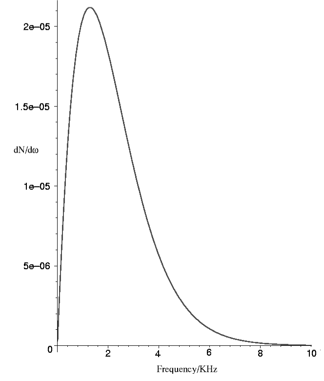
Figure 1: Number spectrum, equation (95), as phonons per 1000 cubic microns per unit out frequency. We have set $c_{f}=10$mm/s and $a_{sf}^{2}/a_{si}^{2}\sim 10$. The typical timescale $t_{0}$ is conservatively set equal to $10^{-3}$s.

The total number of phonons emitted is given by

$$N={1\over 16\pi^{5}}{V\over(c_{sf}t_{0})^{3}}\left({a_{sf}^{4}+a_{si}^{4}\over a_{sf}^{2}a_{si}^{2}}\right)^{3}\;\int_{0}^{\infty}x^{2}\;{\sinh^{2}[x(a_{sf}^{2}/a_{si}^{2}-1)/2]\over\sinh[x(a_{sf}^{2}/a_{si}^{2})]\;\sinh[x]}\;{\mathrm{d}}x={1\over 16\pi^{5}}{V\over(c_{sf}t_{0})^{3}}\left({a_{sf}^{4}+a_{si}^{4}\over a_{sf}^{2}a_{si}^{2}}\right)^{3}F(a_{sf}^{2}/a_{si}^{2}),$$ (96)

so qualitatively we have the same behaviour as in the adiabatic approximation, modulated by a dimensionless function of the ratio $a_{sf}/a_{si}$. (This expression will remain valid as long as $\eta_{0}$ is longer than the healing time; at which stage one should switch over to the sudden approximation.) Using hyperbolic trig identities the previous integral can be re-written as

$$F(z)={1\over 2}\int_{0}^{\infty}x^{2}\left\{\coth(zx)\;\coth(x)-1-{1\over\sinh(zx)\;\sinh(x)}\right\}\;{\mathrm{d}}x$$ (97)

with

$$F(1)=0;\qquad F(\infty)={\zeta(3)\over 4}\approx 0.3005;\qquad\hbox{and}\qquad F(1/z)=z^{3}F(z).$$ (98)

For $z>1$ the function $F(z)$ quickly and smoothly approaches its asymptotic value.

In closing our analysis of the intermediate regime we want now to compare the exact spectrum equation (95) with the spectrum obtained within the adiabatic approximation. Equation (82) can be easily rewritten in the laboratory variables as

$${{\mathrm{d}}N\over{\mathrm{d}}\omega^{t}_{out}}={V\over{2\pi^{2}}}\frac{1}{\exp\left[4\pi\frac{\textstyle a^{2}_{sf}a^{2}_{si}}{\textstyle a^{4}_{si}+a^{4}_{sf}}\omega^{t}_{out}t_{0}\right]-1}\frac{(\omega^{t}_{out})^{2}}{c_{sf}^{3}}.$$ (99)

The combined plot of (95) and (99) is shown in figure 2.

Figure 2: Comparison of the exact number spectrum, equation (95) darker line in the graph, with the one obtained in the adiabatic approximation, equation (99). Both the spectra are shown as phonons per 1000 cubic microns per unit out frequency. In both the cases we have set $c_{f}=10$mm/s and $a_{sf}^{2}/a_{si}^{2}\sim 10$. The typical timescale $t_{0}$ is conservatively set equal to $10^{-3}$s.

It is evident that apart from a minor discrepancy at lower frequencies the two plots basically coincide from the peak frequency (approximately 2 kHz) on. This is not so surprising given that the adiabatic approximation implies $\eta_{0}ka_{sf}^{2}\gg 1$ which in laboratory variables corresponds to

$$2\frac{\textstyle a^{2}_{si}a^{2}_{sf}}{\textstyle a^{4}_{si}+a^{4}_{sf}}\omega^{t}_{out}t_{0}\gg 1.$$ (100)

One can easily check that this inequality starts to be satisfied for frequencies of the order of a few kHz (and holds for any larger frequency).

IV.3 Observability of the effect

In this subsection we will calculate the relevant ratio $C$ defined in equation (45). We want $C\geq 1/100$ to make the phonons easily detectable. By using equation (16) we can deduce that

$$C={1\over N_{c}}\int dx^{3}\left({1\over 4n_{c}}\langle\widehat{n}_{1}\widehat{n}_{1}\rangle+{n_{c}\over\hbar^{2}}\langle\widehat{\theta}_{1}\widehat{\theta}_{1}\rangle-i{1\over 2\hbar}\langle[\widehat{n}_{1},\widehat{\theta}_{1}]\rangle\right).$$ (101)

In the acoustic regime and for the particular configurations we are looking at we know that $\kappa\widehat{n}_{1}=-\partial_{t}\widehat{\theta}_{1}$. Considering now that $[\widehat{n}_{1}(x,t),\widehat{\theta}_{1}(y,t)]=i\hbar\;\delta^{3}(x-y)$ or $[\widehat{\theta}_{1}(x,t),\partial_{t}\widehat{\theta}_{1}(y,t)]=i\hbar\;\kappa\;\delta^{3}(x-y)$ — we can deduce this starting from the fundamental commutation relation $[\widehat{\Psi}^{\dagger}(x,t),\widehat{\Psi}(y,t)]=\delta^{3}(x-y)$)— we can arrive at

$$C={1\over N_{c}}\int dx^{3}\left({1\over 4n_{c}\kappa^{2}}\langle\partial_{t}\widehat{\theta}_{1}\partial_{t}\widehat{\theta}_{1}\rangle+{n_{c}\over\hbar^{2}}\langle\widehat{\theta}_{1}\widehat{\theta}_{1}\rangle+{1\over 2}\delta(0)\right).$$ (102)

To calculate this average, we can expand the real field operator $\widehat{\theta}_{1}$ in terms of the creation and annihilation operators associated with the final configuration

$$\widehat{\theta}_{1}(y,t)=\int dk^{3}{(\hbar\kappa)^{1/2}\over(2\pi)^{3/2}(2\omega(k))^{1/2}}\;a_{k}\;e^{-i\omega t+i{\mathbf{k}}\cdot{\mathbf{x}}}+{\rm H.C.}$$ (103)

and consider the appropriate particle content for the quantum state. If $N_{k}$ is the average number of particles with momentum $k$ in the quantum state, the previous magnitude can be expressed as

$$C= {1\over 2N_{n}\;(n_{c}\kappa)}\int\hbar\omega(k)\;N_{k}dk^{3}+2{(n_{c}\kappa)\over N_{c}}\int{1\over\hbar\omega(k)}N_{k}dk^{3}$$ (104)

$$= {1\over 2N_{c}\;(mc_{s}^{2})}\int\hbar\omega(k)\;N_{k}dk^{3}+2{mc_{s}^{2}\over N_{c}}\int{1\over\hbar\omega(k)}N_{k}dk^{3}.$$ (105)

To reach this expression we have to substract the vacuum contribution. If we consider now the sudden approximation to calculate this rate (an upper limit to what one could get) we obtain

$$C=\left\{{3\over 8}{\hbar\omega_{\rm heal}\over mc_{s}^{2}}+3{mc_{s}^{2}\over\hbar\omega_{\rm heal}}\right\}\;{N\over N_{c}},$$ (106)

with $N$ the one in equation (79). Now $\hbar\omega_{\rm heal}\simeq 10^{-10\pm 1}$ eV. Instead $mc_{s}^{2}\simeq{\rm atomic\;number}\times 10^{-13\pm 1}$ eV $\simeq 10^{-11\pm 1}$ eV. The factor $\hbar\omega_{\rm heal}/mc^{2}\simeq 10$, so we have that the relevant number $C\simeq 4N/N_{c}$. But $N_{c}\simeq 10^{6}$ and $N\simeq 10^{4}-10^{7}$. This gives $C\simeq 4\times 10^{-2}-40$. This number is based on the sudden approximation and will be smaller in a more realistic calculation. However, remembering the discussion on the adiabatic approximation we know that, for temporal scales of change $t_{0}$ of the order of the healing time, the actual coefficient $C$ cannot be smaller than $0.1$ times the previous estimate, i.e. $C\simeq 4\times 10^{-3}-4$. Therefore, by implementing in laboratory an expansive process with $t_{0}$ in an intermediate regime, in between the healing times $t_{\rm heal}=\xi/c_{s}$ associated with the initial configuration ($t_{0}\simeq 10^{-5}$ seconds) and the final configuration ($t_{0}\simeq 10^{-3}$ seconds), one should be able to observe the effect.

V Summary and Discussion

In this work we have discussed the possibilities that BECs offer for simulating Lorentzian geometries of the cosmological type in the laboratory. There are two inequivalent paths one can follow in this task. The first one is based on provoking an expansive explosion in the condensate by changing with time the characteristic frequency of an isotropic and harmonic confining potential. This option implies that the velocity profile of the condensate acquires arbitrarily high values at large distances from the center. So there is always a sphere at which the velocity of the expanding BEC would surpass its sound velocity: A sonic horizon would be formed. In practice, due to the fact that physically realizable BECs are finite systems, one can only reproduce on them a portion of an expanding universe. Therefore one might argue that the sonic horizon would be formed outside the BEC. However, the velocity of sound in BECs is so small (a few mm/s) that in practical situations the sonic horizon will be formed well inside the system. Now the existence of sonic horizons is certainly interesting in its own right, but is not inherent to the simulation of cosmological spacetimes. Moreover, the plausible dynamical instabilities associated with their formation could mask the observation of purely cosmological effects.

The alternative path to simulating a cosmological geometry that we have pursued in this article is to take advantage of the possibility of varying the scattering length or, what is the same, the interaction strength between the atoms in the condensate. In this case, what we need is a confining potential with a sufficiently large almost flat minimum in which a portion of the condensate stays at rest. In this configuration, there is no formation of sonic horizons and thus we think it is (both conceptually and technically) a much cleaner path to follow.

The description of the condensation phenomenon naturally involves the separation of the system into a “classical” wave function (the condensate part) and quantum fluctuations. In the acoustic approximation we can think of these quantum fluctuations as phonons over a classical background geometry, in this case, the analogue of a cosmological spacetime. Therefore, we can use the tuning of the scattering length to simulate not only a classical cosmologically expanding universe, but the quantum phenomenon of cosmological particle creation. We have analyzed this well known process by using a minor variant of Parker’s model for a finite amount of expansion Parker . Then, by working with numerical estimates appropriate to currently accessible BECs in dilute gases, we have presented an analysis of the feasibility of observing the effect in real experiments.

We have seen that there is a more than plausible window for the observability of the effect with current technology. In current BECs the scattering length can easily be varied from a 100 nm to 1 nm. This produces an expansion in the geometrical scale factor of about three times. The temporal scale of change of the scattering length cannot be arbitrarily short. It has to be slower than the time scale in which the interaction between two atoms proceeds. We have calculated this time scale to be of the order of microseconds. However, we have also seen that, by driving the previous finite amount of expansion in a temporal scale of change of about fractions of millisecond, one could start to detect the presence of cosmological particle creation. From here one could shorten the time scale down to tens of microsecond progressively amplifying the expected effect. By the time one reaches tens of microseconds the effect would have been amplified by a factor of a hundred, (with timescale still above the interaction time), opening even the possibility of totally disrupting the condensate.

The relevant temporal scales of change for the effect to be observable are of the order of the healing time in the condensate. Therefore we expect that apart from the phonon spectrum calculated by neglecting the modified dispersion relations at high energies, there will be also some production of quasiparticles. To observe the purely cosmological effect one would have to keep this quasiparticle production under a certain level; thus, the temporal scale of change should not be driven significantly beyond the healing time.

In our analysis we have neglected finite volume effects. However we shall now show that these effects are insignificant for the typical condensate we considered here. The fractional change in the number of particles produced due to finite volume effects is expected to be of order $1/(K_{\rm heal}R)=\xi/(2\pi R)$=(cutoff wavelength)/($2\pi\times$size of the condensate). The ratio between the healing length and the BEC Thomas–Fermi radius can be expressed as a ratio between the harmonic trap length and the scattering length.

$$\frac{R}{\xi}=\frac{2\sqrt{\pi}}{15^{1/10}}\left(\frac{N_{c}a}{a_{ho}}\right)^{2/5}.$$ (107)

For a harmonic oscillator length of about $10$ microns, $N_{c}\approx 10^{6}$ atoms and a scattering length of 1 nanometer one gets $R\approx 17\xi$. For a scattering length ten times larger (easily achievable with a Feshbach resonance and still compatible with $N_{c}a^{3}\ll 1$) and $a_{ho}\approx 1\;\mu$m one would get $R\approx 100\xi$. This implies that $\xi/(2\pi R)\leq 1\%$ and hence finite volume effects are negligible.

To conclude, our analysis suggest that it should be already possible to observe the process of cosmological particle creation in BEC analogue systems, by changing the scattering length from an initial value of about 100 nm to a final value of about 1 nm on times scales shorter than milliseconds but larger than tens of microseconds.

References

- (1) N. D. Birrell and P. C. Davies, “Quantum Fields In Curved Space,” Cambridge University Press, Cambridge 1982.
- (2) A. Strominger and C. Vafa, “Microscopic Origin of the Bekenstein-Hawking Entropy,” Phys. Lett. B 379, 99 (1996) [arXiv:hep-th/9601029].
- (3) B. L. Hu and E. Verdaguer, “Stochastic gravity: A primer with applications,” Class. Quant. Grav. 20, R1 (2003) [arXiv:gr-qc/0211090].
- (4) B. L. Hu and E. Verdaguer, “Recent advances in stochastic gravity: Theory and issues,” arXiv:gr-qc/0110092.
- (5) R. Parentani, “What did we learn from studying acoustic black holes?,” Int. J. Mod. Phys. A 17, 2721 (2002) [arXiv:gr-qc/0204079].
-
(6)
W. G. Unruh,
“Notes On Black Hole Evaporation,”
Phys. Rev. D 14, 870 (1976).
W. G. Unruh, “Experimental black hole evaporation?”, Phys. Rev. Lett, 46, 1351 (1981). - (7) M. Visser, “Acoustic black holes: Horizons, ergospheres, and Hawking radiation,” Class. Quant. Grav. 15 (1998) 1767 [arXiv:gr-qc/9712010].
- (8) J. Martin and R. H. Brandenberger, “The trans-Planckian problem of inflationary cosmology,” Phys. Rev. D 63, 123501 (2001) [arXiv:hep-th/0005209].
- (9) L. J. Garay, J. R. Anglin, J. I. Cirac and P. Zoller, “Black holes in Bose-Einstein condensates,” Phys. Rev. Lett. 85, 4643 (2000) [arXiv:gr-qc/0002015].
- (10) L. J. Garay, J. R. Anglin, J. I. Cirac and P. Zoller, “Sonic black holes in dilute Bose-Einstein condensates,” Phys. Rev. A 63, 023611 (2001) [arXiv:gr-qc/0005131].
- (11) C. Barceló, S. Liberati and M. Visser, “Analog gravity from Bose-Einstein condensates,” Class. Quant. Grav. 18 (2001) 1137 [arXiv:gr-qc/0011026].
- (12) M. Novello, M. Visser and G. Volovik, “Artificial Black Holes”, (World Scientific, Singapore, 2002).
- (13) C. Barceló, S. Liberati and M. Visser, “Towards the observation of Hawking radiation in Bose-Einstein condensates,” Int. J. Mod. Phys. A, in press; arXiv:gr-qc/0110036.
- (14) C. Barceló, S. Liberati and M. Visser, “Analogue models for FRW cosmologies”, Int. J. Mod. Phys. D, in press; arXiv:gr-qc/0305061.
-
(15)
E. A. Calzetta and B. L. Hu,
“Bose-Novae as Squeezing of the Vacuum by Condensate Dynamics,”
arXiv:cond-mat/0208569.
E. A. Calzetta and B. L. Hu, “Bose-Novae as Squeezing of Vacuum Fluctuations by Condensate Dynamics,” arXiv:cond-mat/0207289. -
(16)
E. Donley et al., Nature 412 (2001) 295;
N. R. Claussen, Ph. D. Thesis, U. of Colorado (2003). -
(17)
S. L. Cornish, N. R. Claussen, J. L. Roberts, E. A. Cornell, C. E. Wieman,
“Stable 85Rb Bose-Einstein Condensates with Widely Tunable Interactions”
Phys. Rev. Lett 85, 1795 (2000).
arXiv:cond-mat/0004290
J. L. Roberts, N. R. Claussen, S. L. Cornish, E. A. Donley, E. A. Cornell, C. E. Wieman, “Controlled Collapse of a Bose-Einstein Condensate” arXiv:cond-mat/0102116
Elizabeth A. Donley, Neil R. Claussen, Simon L. Cornish, Jacob L. Roberts, Eric A. Cornell, Carl E. Wieman, “Dynamics of collapsing and exploding Bose-Einstein condensates” arXiv:cond-mat/0105019 - (18) A. Griffin, “Conserving and gapless approximations for an inhomogeneous Bose gas at finite temperature” Phys. Rev B53, 9341 (1996).
-
(19)
P. O. Fedichev and U. R. Fischer,
“’Cosmological’ particle production in oscillating ultracold Bose gases:
The role of dimensionality,”
arXiv:cond-mat/0303063;
“Hawking radiation from sonic de Sitter horizons in expanding Bose-Einstein-condensed gases,” arXiv:cond-mat/0304342;
“Observing quantum radiation from acoustic horizons in linearly expanding cigar-shaped Bose-Einstein condensates,” arXiv:cond-mat/0307200 - (20) Y. Kagan, E. L. Surkov and G. V. Shlyapnikov, “Evolution of a Bose-condensed gas under variations of the confining potential,” Phys. Rev. A54, R1753 (1996); Y. Castin and R. Dum, “Bose-Einstein Condensates in Time Dependent Traps,” Phys. Rev. Lett. 77, 5315 (1996).
- (21) Y. Kagan, E. L. Surkov and G. V. Shlyapnikov, “Evolution and global collapse of trapped Bose condensates under variations of the scattering length,” Phys. Rev. Lett. 79, 2604 (1997) [arXiv:physics/9705005].
- (22) G.E. Volovik, “Induced Gravity in Superfluid 3He,” J.Low.Temp.Phys. 113, 667 (1997) [arXiv:cond-mat/9806010].
- (23) Yvan Castin, “Bose-Einstein condensates in atomic gases: simple theoretical results” in ’Coherent atomic matter waves’, Lecture Notes of Les Houches Summer School, p.1-136, edited by R. Kaiser, C. Westbrook, and F. David, EDP Sciences and Springer-Verlag (2001).
- (24) M. Visser, C. Barcelo and S. Liberati, “Acoustics in Bose-Einstein condensates as an example of broken Lorentz symmetry,” arXiv:hep-th/0109033.
- (25) T. Köhler and K. Burnett, “Microscopic quantum dynamics approach to the dilute condensed Bose gas”, Phys. Rev. A65, 033601 (2002).
- (26) G. F. Gribakin and V. V. Flambaum, “Calculation of the scattering length in atomic collisions using the semiclassical approximation”, Phys. Rev. A48, 546 (1993).
- (27) J. Weiner, V. S. Bagnato, S. Zilio, and P.S. Julienne, “Experiments and theory in cold and ultracold collisions” Rev. Mod. Phys. 71, 1 (1999).
- (28) C. J. Williams et al, “Determination of the scattering lengths of from photoassociation line shapes”, Phys. Rev. A60, 4427 (1999).
- (29) E. L. Bolda, E. Tiesinga, and P. S. Julienne, “Effective-scattering-length model of ultracold atomic collisions and Feshbach resonances in tight harmonic traps” Phys. Rev. A66, 013403 (2002).
- (30) L. Parker, “Thermal radiation produced by the expansion of the universe”, Nature 261, 20 (1976).
- (31) C. Eckart, “The penetration of a potential barrier by electrons” Phys. Rev. 35, 1303 (1930).
- (32) S. Liberati, M. Visser, F. Belgiorno and D. W. Sciama, “Sonoluminescence as a QED vacuum effect. I: The physical scenario,” Phys. Rev. D 61, 085023 (2000) [arXiv:quant-ph/9904013].
- (33) S. Liberati, M. Visser, F. Belgiorno and D. W. Sciama, “Sonoluminescence as a QED vacuum effect. II: Finite volume effects,” Phys. Rev. D 61 (2000) 085024 [arXiv:quant-ph/9905034].
- (34) M. Visser, “Some general bounds for 1-D scattering,” Phys. Rev. A 59 (1999) 427 [arXiv:quant-ph/9901030].