Anisotropic Diffusion Limited Aggregation

Abstract

Using stochastic conformal mappings we study the effects of anisotropic perturbations on diffusion limited aggregation (DLA) in two dimensions. The harmonic measure of the growth probability for DLA can be conformally mapped onto a constant measure on a unit circle. Here we map $m$ preferred directions for growth of angular width $\sigma$ to a distribution on the unit circle which is a periodic function with $m$ peaks in $[-\pi,\pi)$ such that the width $\sigma$ of each peak scales as $\sigma\sim 1/\sqrt{k}$, where $k$ defines the “strength” of anisotropy along any of the $m$ chosen directions. The two parameters $(m,k)$ map out a parameter space of perturbations that allows a continuous transition from DLA (for $m=0$ or $k=0$) to $m$ needle-like fingers as $k\to\infty$. We show that at fixed $m$ the effective fractal dimension of the clusters $D(m,k)$ obtained from mass-radius scaling decreases with increasing $k$ from $D_{DLA}\simeq 1.71$ to a value bounded from below by $D_{min}=3/2$. Scaling arguments suggest a specific form for the dependence of the fractal dimension $D(m,k)$ on $k$ for large $k$, form which compares favorably with numerical results.

I Introduction

Nonequilibrium growth models leading naturally to self-organized fractal structures, such as diffusion limited aggregation (DLA) WS81 , have received great interest in the recent years not only due to their relevance for various physical processes, for example dielectric breakdown NPW84 , electrochemical deposition BB84 ; MSHHS84 , and two-fluid Laplacian flow P84 , but also because such harmonic growth leads naturally to one of the most interesting multifractal distributions found in nature HP83 ; HMP86 .

A powerful method for studying such two dimensional growth processes is the iterated stochastic conformal mapping HL98 ; H97 ; DHOSS99 , which has already been successfully applied to generate and analyze DLA DHOSS99 ; DP00 and Laplacian BDLP00 growth patterns in two dimensions. This has opened the road to address many important questions related to pattern formation in DLA, such as the structure of the multifractal spectrum of DLA JLMP02 , and provided the first definite answers for how the hottest tips and the coldest fjords grow. Other topics that can be investigated using iterated conformal maps include the pinning transition in Laplacian growth HPF02 , the difference between Hele-Shaw flows and DLA HLP02 , as well as new topics such as the scaling of fracture surfaces formed during quasistatic cracking BHLP02 .

One of the important questions addressed soon after the original discovery of DLA by Witten and Sander WS81 was that of the effect of the intrinsic anisotropy in lattice models on the shape and fractal dimension of the asymptotic aggregates BBRT85_86 ; M88 ; EMPZ89_90 ; AACR91 ; JS95 . For two dimensional growth, it was shown that the result of such anisotropy in the microscopic attachment probability leads to clusters which asymptotically have the symmetry of the underlying lattice (following the argument in Ref BBRT85_86 , this actually holds for $m\leq 6$, where $m$ represents the coordination number of the lattice), and the fractal dimension of the resulting aggregate asymptotically approaches $3/2$. These results have also been confirmed in recent work which used iterated stochastic conformal mapping techniques to grow the clusters SL01 .

In the present work we use iterated stochastic conformal mapping techniques to study DLA with $m$ preferred directions for growth. Although this naturally leads to anisotropic clusters, the present model is fundamentally different from the previous studies on lattice anisotropy. Our model is rather related to the existence of a large scale imposed $m$-fold symmetry whose strength can be tuned. Specifically let us consider the case when the harmonic measure for DLA is weighted at angle $\psi$ between the seed and the location for growth by a term $W(\psi;m,\sigma)$, where $\sigma$ specifies the angular width of the preferred direction. Such a weighting $W(\psi;m,\sigma)\sim\exp[-\beta{\cal H}(\psi;m,\sigma)]$ could be due to an imposed external field or to growth on a surface which has an $m$ fold symmetry. An example would be dendritic growth in a strip AACR91 which can be argued to lie in the $m=1$ or $m=2$ universality class, the anisotropy increasing as the strip is narrowed.

The organization of the paper is as follows. In Section II we describe how we use conformal mapping methods together with an angle dependent probability for growth $P(\theta;m,k)$ to study a model corresponding to a real space weighting $W(\psi;m,\sigma)$. Here $\theta$ is the angle parametrising the unit circle to which the boundary of the growing cluster is conformally mapped, $m$ is the number of the privileged directions, and $k$ is an appropriate measure for the “strength” of the anisotropy. In Section III we present results for the morphology of the resulting patterns as a function of $m$ and $k$, and we derive using scaling arguments the effective fractal dimension $D(m,k)$ of the emerging clusters. We conclude with a discussion of the results in Section IV.

II Model and Theoretical Background

In the DLA model proposed by Witten and Sander WS81 the growth of a cluster from a seed placed at the origin proceeds by irreversible attachment of random walkers released from infinity (in practice, from far away from the cluster’s boundary). Thus the probability $P(s)$ for growth at any point $s$ along the cluster boundary of total length $L$ is a harmonic measure and can be written $P(s)=|(\nabla V)(s)|/\int_{0}^{L}|(\nabla V)(s^{\prime})|ds^{\prime}$, where $V({\bf r})$ is a potential which outside the cluster obeys Laplace’s equation $\nabla^{2}V=0$ subject to the boundary conditions $V=0$ on the (evolving) boundary of the cluster and $V\sim\ln r$ as $r\to\infty$ (corresponding to a uniform source of particles far away from the cluster). In two dimensions, this formulation as a potential problem has been recently exploited for studying the time development of DLA based on conformal mapping techniques  HL98 ; DHOSS99 .

As discussed in detail in  HL98 ; DHOSS99 , the basic idea is to follow the evolution of the conformal mapping $\Phi^{(n)}(\omega)$ of the exterior of the unit circle in a mathematical $\omega$–plane onto the complement of the cluster of $n$ particles in the physical $z$–plane rather than directly the evolution of the cluster’s boundary. The equation of motion for $\Phi^{(n)}(\omega)$ is determined recursively (see Fig. 1(a)). With an initial condition corresponding to the unit circle in the physical plane $\Phi^{(0)}(\omega)=\omega$, the process of adding a new “particle” of constant shape and linear scale $\sqrt{\lambda_{0}}$ to the cluster of $(n-1)$ “particles” at a position $s$ chosen according to the harmonic measure is performed using an elementary mapping $\phi_{\lambda,\theta}(\omega)$

$$\phi_{\lambda,0}(\omega)=\omega^{1-a}\left\{\frac{(1+\lambda)}{2\omega}(1+\omega)\right.$$

$$\left.\times\left[1+\omega+\omega\left(1+\frac{1}{\omega^{2}}-\frac{2}{\omega}\frac{1-\lambda}{1+\lambda}\right)^{1/2}\right]-1\right\}^{a}$$

$$\phi_{\lambda,\theta}(\omega)=e^{i\theta}\phi_{\lambda,0}(e^{-i\theta}\omega)\,,$$ (1)

which conformally maps the unit circle to the unit circle with a bump of size $\sqrt{\lambda}$ localized at the angular position $\theta$  HL98 . The parameter $a$ describes the shape of the elementary mapping; following the analysis in  DHOSS99 , we have used $a=0.66$ throughout this paper as we believe the large scale asymptotic properties will not be affected by the microscopic shape of the added bump. As shown diagrammatically in Fig. 1(a), the recursive dynamics can than be represented as iterations of the elementary bump map $\phi_{\lambda_{n},\theta_{n}}(\omega)$, resulting in the convolution representation of the conformal map $z=\Phi^{(n)}(\omega)$ at the $n$th stage of growth as

$$\Phi^{(n)}(\omega)=\phi_{\lambda_{1},\theta_{1}}\circ\phi_{\lambda_{2},\theta_{2}}\circ\dots\circ\phi_{\lambda_{n},\theta_{n}}(\omega)\,,$$ (2)

where the angle $\theta_{n}\in[-\pi,\pi)$ at step $n$ is randomly chosen because the harmonic measure on the real cluster translates to a uniform measure on the unit circle in the mathematical plane, i.e,

$$P(s)ds=\frac{d\theta}{2\pi}.$$ (3)

Eq. 3 is crucial to the successful implementation of the iterated conformal method as the highly nontrivial harmonic measure in the physical plane becomes uniform in the mathematical plane. Finally,

$$\lambda_{n}=\frac{\lambda_{0}}{|{\Phi^{(n-1)}}^{\prime}(e^{i\theta_{n}})|^{2}}$$ (4)

is required in order to ensure that the size of the bump in the physical $z$ plane is $\sqrt{\lambda_{0}}$. We note that in the composition Eq. 2 the order of iterations is inverted – the last point of the trajectory is the inner argument, therefore the transition from $\Phi^{(n)}(\omega)$ to $\Phi^{(n+1)}(\omega)$ is achieved by composing the $n$ former maps Eq. 2 starting from a different point.

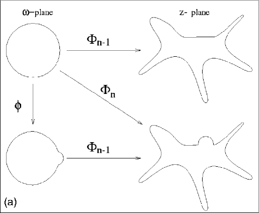
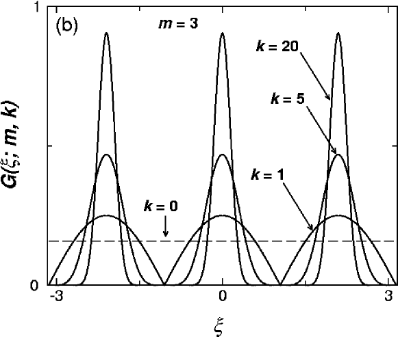
Figure 1: (a) Diagrammatic representation of the mappings $\Phi$ and $\phi$. (b) Change in shape of the probability distribution $G(\xi;m,k)$ with increasing $k$ for $m=3$.

Consider the case where the existence of $m$ preferred directions in physical space modulates the harmonic measure at any point $s$ on the boundary by a probability $P(\psi(s);m,\sigma)=W(\psi(s);m,\sigma)/\int_{0}^{L}W(\psi(s^{\prime});m,\sigma)ds^{\prime}$. Here, $\psi(s)$ is the angle parameterisation of the cluster boundary in the physical space, $W(\psi;m,\sigma)$ is the modulating weight, and the $m$-fold periodicity implies $P(\psi~{}+~{}2\pi/m;m,\sigma)=P(\psi;m,\sigma)$. The important question is if the weighting $W(\psi;m,\sigma)$ in the real space may be represented in the form of a modulation of the constant measure in the mathematical plane $P_{math}(\theta)=d\theta/2\pi$. Because the angle $\psi$ is not invariant under the conformal map $z=\Phi^{(n)}(\omega)$, an answer to the question above is not straightforward. Considering an ensemble of clusters generated under the influence of the same modulation $P(\psi;m,\sigma)$, for each cluster of $n$ particles $\psi$ maps onto a different $\theta_{n}(\psi)$, where $\exp{i\psi}=\Phi^{(n)}(\exp{i\theta_{n}})/|\Phi^{(n)}(\exp{i\theta_{n}})|$. It is reasonable to assume that averaging over the many patterns above an asymptotically ($n\to\infty$) average scale invariant pattern will appear. For DLA, i.e., in the absence of modulation, this pattern is a circle; in the general case, an $m$ fold periodic pattern with the same symmetry as the modulation is expected to appear. Therefore, we expect $\langle\theta_{n}(\psi)\rangle=f_{m}(\psi)$, where $\langle\dots\rangle$ denotes an average over clusters, with $f_{m}(\psi)$ independent of $n$ and satisfying $f_{m}(\psi+2\pi/m)=f_{m}(\psi)+2\pi/m$ due to the symmetry of the resulting averaged pattern and to the fact that $f_{m}$ is an angle. In principle, $f_{m}$ is defined up to an additive constant; this can be fixed by specifically requiring that at the pattern fingertips $j=0,1,2,...m-1$ one has $f_{m}(2\pi j/m)=2\pi j/m$. It then follows that the modulated probability distribution on the unit circle leading to such $m-$fold symmetry patterns obeys

$$P_{math}(\theta)=P(f_{m}^{-1}(\theta);m,\sigma)df_{m}^{-1}(\theta)/d\theta$$ (5)

Thus, we can see that for this case $P_{math}(\theta)$ is itself an $m$-fold periodic function on the unit circle with peaks at the preferred directions $\theta_{k}=2\pi k/m$.

In this paper, rather than attempting to derive a specific $P_{math}(\theta)$ using Eq. 5, we shall directly assume such an $m$-fold periodic measure on the unit circle (which based on the arguments above is expected to lead to an $m-$fold symmetry weighting function $W$ in the physical space) and study the clusters created using the choice $P_{math}(\theta)=G(\theta;m,k)d\theta$, where the parameter $k\sim 1/\sigma$ is an appropriate measure of the angular width of the preferred direction in the physical plane. The angle-dependent probability distribution on the unit circle $G(\theta;m,k)$ will be normalized such that $\int_{-\pi}^{\pi}d\theta\,G(\theta;m,k)=1$. Such a distribution biases the choice of the location $\theta$, and thus $s$, where growth occurs as follows. At step $n$, the point $s$ for the attempt of growth is chosen, as before, based on the harmonic measure, i.e., one chooses points $\theta_{n}\in[-\pi,\pi)$ on the unit circle with uniform distribution. But growth at $s$ is only allowed with a probability $G(\theta_{n};m,k)$. If the attempt is rejected, then the previous sequence is repeated until a successful trial occurs. We note that obviously $G(\theta;m,k)=const$ corresponds to usual DLA, while an explicit dependence on $\theta$ models the existence of privileged directions.

Because at this stage we are interested in the general features of such a model of anisotropic growth, and not in trying to model a specific physical system, we will make the simple choice

$$G(\theta;m,k)=\frac{1}{C(k)}\left|\cos\left(\frac{m}{2}\theta\right)\right|^{k},$$

$$\theta\in{\left[\right.}-\pi,\pi\left.\right),~{}m\in\mathbb{N}~{},~{}k\in\mathbb{R}_{+}~{},$$ (6)

where

$$C(k)=\frac{4\,{\sqrt{\pi}}\,\Gamma(\frac{3}{2}+\frac{k}{2})}{\left(1+k\right)\,\Gamma(1+\frac{k}{2})}$$

is the normalization constant (note that it does not depend on $m$).

It is easy to see that $G(\theta;m,k)$ defined above has all the key properties required: for $m>0$ it is a periodic function of $\theta$ of principal period $2\pi/m$, and thus the number $m$ of peaks of $G(\theta;m,k)$ in $\left[-\pi,\pi\right)$ corresponds to the number of privileged directions; obviously, both $k=0$ independent of $m$ and $m=0$ independent of $k$ correspond to isotropic DLA growth. The exponent $k>0$ is a measure for the “strength” of selectivity, i.e., the larger $k$, the narrower and higher peaks of $G(\theta;m,k)$. Therefore, the pair $(m,k)$ defines a two dimensional parameter space for the analytic study of applied anisotropy to DLA. Though the choice given by Eq. 6 is arbitrary, we believe that because of universality the key features will be independent of the specific form of the function $G(\theta;m,k)$.

III Results and Discussion

The model described in Sec. II was simulated as follows. The parameter $\lambda_{0}=10^{-3}$ was fixed because it is just setting the microscopic area of an added “particle”. For fixed $m$ and $k$ the growth step $n$ proceeds by selecting at random (uniform probability) an angle $\theta\in[-\pi,\pi)$, then comparing $G(\theta;m,k)$ with a random number $r$ uniformly distributed in $[0,1/C(k))$; if $r<G(\theta;m,k)$, then $\theta_{n}=\theta$, $\lambda_{n}$ follows from Eq. 4, and the new map $\Phi_{n}$ follows from Eq. 2; if not, the previous sequence is repeated until a successful trial occurs. All the averages mentioned below were done over $100$ clusters grown up to size $N=20000$. An example of clusters with different symmetries (i.e., different values $m$) grown in this manner is shown in Fig. 2(a), while Fig. 2(b) depicts the morphology with increasing anisotropy “strength” (i.e., different values $k$ at fixed $m$).

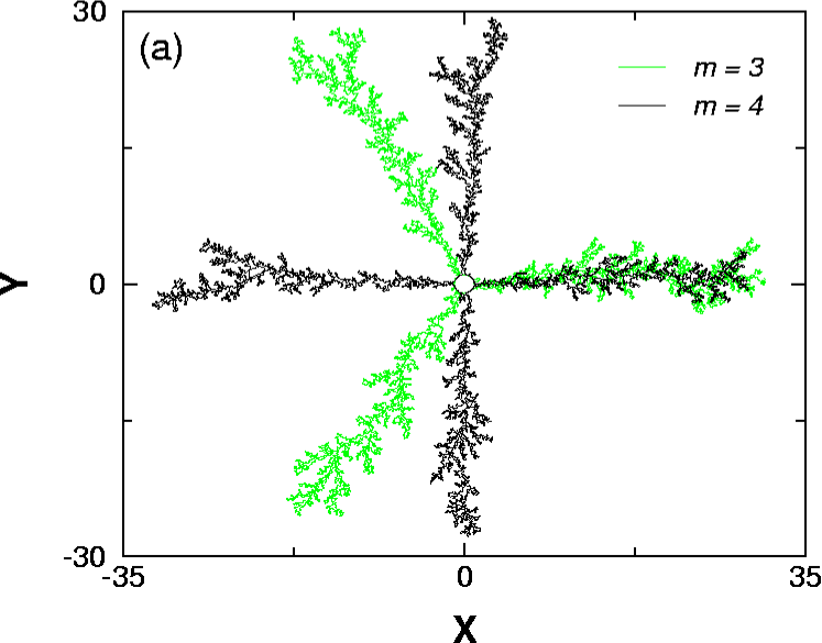
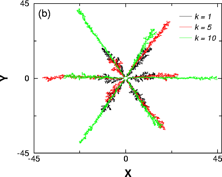
Figure 2: Typical clusters (size $N=20000$) grown with (a) $m=3,4$, fixed $k=3$, and (b) fixed $m=6$, but different values for $k$, $k=1,5,10$, respectively.

It can be seen that the bias introduced by the distribution $G(\theta;m,k)$ is indeed producing clusters with the corresponding $m-$ fold symmetry and that it is very effective: even for small values $k$, the clusters in Fig. 2(a) show a clear 3-fold, respectively 4-fold, symmetry. Increasing $k$ (the strength of the anisotropy) leads to a significant reduction in the branched structure of the cluster, thus in the thickness of the surviving branches, as shown in Fig. 2(b). Similar results have been obtained for all the values $2\leq m\leq 7$ and $1\leq k\leq 80$ that have been tested.

The results shown in Fig. 2 suggest that the resultant patterns have a fractal morphology that depends on $m$ and $k$, and in order to characterize these shapes we will focus on the effective fractal dimension $D(m,k)$ obtained from the mass-radius scaling. Following the arguments in Ref.  DHOSS99 , the coefficient $F^{(n)}_{1}=\Pi_{i=1}^{n}(1+\lambda_{i})^{a}$ in the Laurent expansion of $\Phi^{(n)}$,

$$\Phi^{(n)}(\omega)=F^{(n)}_{1}\omega+F^{(n)}_{0}+F^{(n)}_{-1}\omega^{-1}+F^{(n)}_{-2}\omega^{-2}+\dots~{},$$ (7)

is a typical length-scale of the cluster; thus, a natural choice for the radius of the $n$-particle cluster is $R\sim F_{1}^{(n)}$. Assuming that for $n>>1$ a scaling law of the form

$$F_{1}^{(n)}\sim n^{1/D(m,k)}$$ (8)

is found, the effective fractal dimension of the cluster can be extracted from a power law fit to the numerical data. We note in passing that this scaling law was used in Ref.  DHOSS99 as a very convenient way to measure the fractal dimension of the growing DLA cluster. As we have anticipated, for all the values $m$ and $k$ the numerical results for the average coefficient $F_{1}^{(n)}$ show clear power-law dependence on the size $n$, an example being shown in Fig. 3(a), and the results $D(m,k)$ obtained from the power-law fit to the data in the range $n\geq 10^{3}$ are shown in Fig. 3(b).

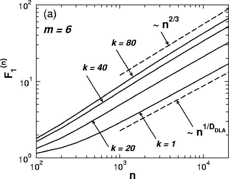
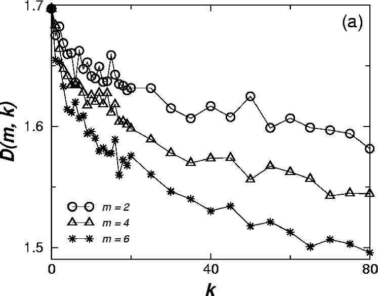
Figure 3: (a) Average $F_{1}^{(n)}$ as a function of $n$ for clusters grown with $k=1,10,40,\textrm{and }80$, respectively, and fixed $m=6$ (log-log plot). Also shown (dashed lines) are both the limit case $F_{1}^{(n)}\sim n^{1/D_{DLA}}$ (DLA cluster), where $D_{DLA}=1.71$, and the proposed lower bound for anisotropic DLA growth  BBRT85_86 $F_{1}^{(n)}\sim~{}n^{1/D_{min}}$, where $D_{min}=3/2$. (b) The effective fractal dimension $D(m,k)$, obtained from $F_{1}^{(n)}\sim n^{1/D(m,k)}$, as a function of $k$ at fixed $m$. The points represent the measured values, the lines are just a guide to the eye.

It can be seen that $D(m,k)$ decreases with increasing $k$ at fixed $m$ (and with increasing $m$ at fixed $k$), and there is a certain tendency for saturation at large $k$. We note that, as expected, $D(m,0)\simeq D_{DLA}$ and that the curves $D(m,k)$ are all above the expected lower limit $D_{min}=3/2$  BBRT85_86 . An exception is the case $m=7$ (results not shown), where for large $k$ the values $D(7,k>>1)\simeq 1.45$ are somewhat below $D_{min}$, but this is most probably due to either insufficient statistics (too few clusters), as suggested also by the noisiness of the $D(m,k)$ curves, or to the fact that in this particular case the size $N=20000$ is not sufficient to obtain an asymptotic cluster.

In order to understand these results theoretically we will use a simple argument, following Ref.  BBRT85_86 , based on the assumptions that (a) for large $k$ the growth of the cluster occurs mainly at the tips of the $m$ principal branches, and (b) the envelope of the average cluster can be approximated by $m$ diamond shaped polygons, like the one shown in Fig. 4(a), of opening angles $\gamma$ and $\beta$ (in general, these angles depend on both $m$ and $k$) and with edges of lengths in the order of $R$.

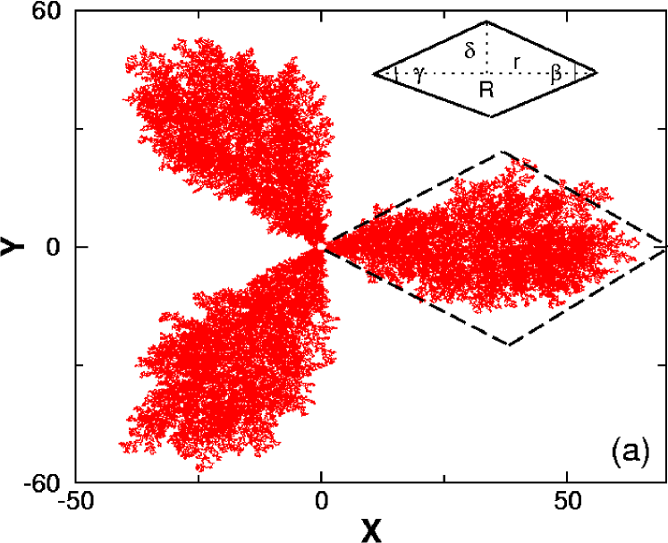
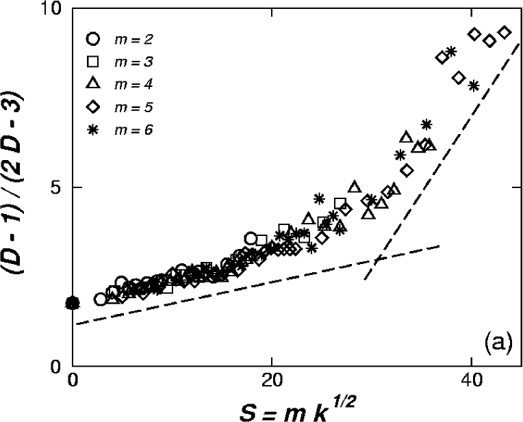
Figure 4: (a). Superposition of $10$ different clusters of size $N=10^{5}$ grown with the same $m=3$ and $k=1$ but different sequences of random numbers. The dotted diamond around the arm centered at $\psi=0$ shows the approximation for the envelope of one arm of the cluster, and the drawing in the upper right corner shows schematically the geometry of the diamond. (b) Numerical results for $\frac{D-1}{2D-3}$ as a function of the scaling variable $S=m\sqrt{k}$. The dashed lines are just a guide to the eye for the linear behavior in the range $S>>1$ and, respectively, $S\gtrsim 1$.

Under these assumptions, the rate of growth can be written as  BBRT85_86

$$dN/dR\sim R^{\pi/(2\pi-\beta)}.$$ (9)

Because the LHS of Eq. 9 is $LHS\sim R^{D(m,k)-1}$, once the angle $\beta(m,k)$ is known $D(m,k)$ can be determined from

$$D(m,k)=1+\frac{\pi}{2\pi-\beta(m,k)}$$ (10)

Simple geometry (see the schematic drawing in the top right corner of Fig. 4(a)) allows one to write (under the assumption that the angles $\gamma(m,k)$ and $\beta(m,k)$ are small – which is certainly true for large $k$ and $m$),

$$\gamma=\frac{\delta}{R-r},~{}\beta=\frac{\delta}{r}~{}\Rightarrow~{}\beta=\frac{R-r}{r}\,\gamma$$ (11)

On the other hand, the opening angle $\gamma(m,k)$ is obviously fixed by the decay of the probability for growth $G(\theta;m,k)$, and therefore can be estimated as the width of the peak of the distribution. Working with the peak centered at $\theta=0$, assuming large $k$ and small $\gamma$, the width at half peak probability is given by $1/2\approx\left[1-\left(m\gamma/4\right)^{2}\right]^{k}\approx 1-k\left(m\gamma/4\right)^{2}$. Thus, from Eq. 11,

$$\gamma(m,k)\approx\frac{2}{m\sqrt{k}}~{}\Rightarrow\beta(m,k)\approx\frac{2(R-r)}{r\,m\sqrt{k}}=\frac{C_{1}}{m\sqrt{k}}$$ (12)

where $C_{1}$ is a constant of ${\cal O}(1)$, independent of $m$, $k$, or the size $N$ of the cluster. Combining Eqs. 10 and 12, one thus obtains the following scaling relation for the fractal dimension

$$\frac{D(m,k)-1}{2D(m,k)-3}=\frac{\pi}{C_{1}}m\sqrt{k}.$$ (13)

Note that it is immediately apparent from Eq. 13 that $D_{min}=3/2$, while for large $k$ the ratio $(D-1)/(2D-3)$ should be a linear function of the product $S=m\sqrt{k}$ only, provided $S>>1$. This prediction can be tested against the numerical results. As shown in Fig. 4(b), the data collapse is excellent and the function is indeed linear when $S>>1$, confirming our theory. Surprisingly, the scaling predicted by Eq. 13 seems to hold down to quite small values of $k$, although these results are beyond the scope of our scaling arguments.

IV Conclusions

Using iterated stochastic conformal maps, we have studied the patterns emerging from a model of anisotropic (in the sense of the existence of privileged radial directions for growth) diffusion limited aggregation in two dimensions. In our model, the anisotropy was introduced via a probability distribution for growth with a number $m$ of peaks in $[-\pi,\pi)$, the width of a peak (giving the “strength” of anisotropy) being a tunable parameter that allows a continuous transition from isotropic DLA growth to anisotropic clusters. We have shown numerical evidence that at fixed $m$ the effective fractal dimension of the clusters $D(m,k)$ obtained from the mass-radius scaling decreases with $k$ from $D_{DLA}$ to values bounded from below by $D_{min}=3/2$. Using simple approximations (supported by numerical results) for the envelope of the cluster and general scaling arguments, we have derived a scaling law involving $D(m,k)$ and successfully tested it against numerical results.

Although the model we have proposed is somewhat artificial, it has the advantage that it seems to capture most of the general features of an anisotropic growth process while it is still simple enough to allow an analytical treatment (to a certain degree). Finally, we note here that a system for which the proposed geometry may be easily experimentally achieved is the growth of bacterial colonies. For such a case, the radial anisotropy can be experimentally obtained through the addition of nutrients along the privileged directions, and controlled through the excess concentration of nutrients along these directions in respect to the rest of the substrate. This would allow a direct testing of all our numerical and analytical predictions.

- (1) T.A. Witten Jr. and L.M. Sander, Phys. Rev. Lett. 47,1400 (1981).
- (2) L. Niemeyer, L. Pietronero, and H.J. Wiesmann, Phys. Rev. Lett. 52,1033 (1984).
- (3) R.M. Brady and R.C. Ball, Nature 309, 225 (1984).
- (4) M. Matshushita, M. Sano, Y. Hayakawa, H. Honjo, and Y. Sawada, Phys. Rev. Lett. 53,286 (1984).
- (5) L. Paterson, Phys. Rev. Lett. 52,1621 (1984).
- (6) H.G.E. Hentschel and I. Procaccia, Physica D 8, 435 (1983).
- (7) T.C. Halsey, P. Meakin and I. Procaccia, Phys. Rev. Lett. 56, 854 (1986).
- (8) M.B. Hastings and L.S. Levitov, Physica D 116, 244 (1998).
- (9) M.B. Hastings, Phys.Rev.E 55, 135 (1997).
- (10) B. Davidovich, H.G.E. Hentschel, Z. Olami, I.Procaccia, L.M. Sander, and E. Somfai, Phys. Rev. E 59, 1368 (1999).
- (11) B. Davidovich and I. Procaccia, Phys. Rev. Lett. 85, 3608 (2000).
- (12) F. Barra, B. Davidovitch, A. Levermann, and I. Procaccia, Phys. Rev. Lett. 87, 134501 (2001).
- (13) M.H. Jensen, A. Levermann, J. Mathiesen, and I. Procaccia, Phys. Rev. E 65, 046109 (2002).
- (14) H.G.E. Hentschel, M.N. Popescu, and F. Family, Phys. Rev. E 65, 036141 (2002).
- (15) H.G.E. Hentschel, A. Levermann, and I. Procaccia, Phys. Rev. E 66, 016308 (2002).
- (16) F. Barra, H.G.E. Hentschel, A. Levermann, and I. Procaccia, Phys. Rev. E65, 045101 (2002).
- (17) R.C. Ball, R.M. Brady, G. Rossi, and B.R. Thompson Phys. Rev. Lett. 55, 1406 (1985); R.C. Ball, Physica 140A, 62 (1986).
- (18) P. Meakin, in Phase Transitions and Critical Phenomena, edited by C. Domb and J. Lebowitz (Academic, New York, 1988), Vol. 12.
- (19) J.P. Eckmann, P. Meakin, I. Procaccia, and R. Zeitak, Phys. Rev. A 39, 3185 (1989); ibid, Phys. Rev. Lett. 65, 52 (1990).
- (20) A. Arnedo, F. Argoul, Y. Couder, and M. Rabaud, Phys. Rev. Lett. 66, 2332 (1991).
- (21) B.K. Johnson and R.F. Sekerka, Phys. Rev. E 52, 6404 (1995).
- (22) M.G. Stepanov and L.S. Levitov, Phys. Rev. E 63, 061102 (2001).
- (23) L. Turkevich and H. Sher, Phys. Rev. Lett. 55, 1026 (1985).