On the effect of far impurities on the density of states of 2DEG in a strong magnetic field On the Effect of Far Impurities on the Density of States of Two-Dimensional Electron Gas in a Strong Magnetic Field

I. S. Burmistrov and M. A. Skvortsov Burmistrov, Skvortsov

On the Effect of Far Impurities on the Density of States of Two-Dimensional Electron Gas in a Strong Magnetic Field

Abstract

The effect of impurities situated at different distances from a two-dimensional electron gas on the density of states in a strong magnetic field is analyzed. Based on the exact result of Brezin, Gross, and Itzykson, we calculate the density of states in the whole energy range, assuming the Poisson distribution of impurities in the bulk. It is shown that in the case of small impurity concentration the density of states is qualitatively different from the model case when all impurities are located in the plane of the two-dimensional electron gas.

73.43 -f

1. Introduction. Two-dimensional electrons in a quantizing magnetic field $H$ has been attracting much attention [1] especially since the discovery of the quantum Hall effect [2]. The properties of two-dimensional electrons in the magnetic field are affected by the presence of electron-electron interaction as well as by impurities. Investigation of the density of states as a function of the magnetic field and filling fraction allows us to estimate the inhomogeneities caused by impurities in experimental samples [3]. Although the electron-electron interaction should usually be taken into account, the question about the density of states in the simplest model of noninteracting electrons is also rather interesting.

In the absence of interaction, impurities near a two-dimensional electron gas (2DEG) provide the only mechanism for broadening of Landau levels. In a weak magnetic field the large number of Landau levels, $N\gg 1$, are filled. One can therefore use the self-consistent Born approximation that is justified by the small parameter $\ln N/N\ll 1$. It results in the well-known semicircle shape for the density of states [4]. Beyond the self-consistent Born approximation one can find the exponentially small tails in the density of states [5].

In the opposite limit of a strong magnetic field only the lowest Landau level is partially occupied. In this case one can neglect the influence of the other empty Landau levels assuming $\omega_{H}\gg T,\tau^{-1}$. Here $\omega_{H}=eH/m$ denotes the cyclotron frequency with $e$ and $m$ being the electron charge and mass respectively, $T$ stands for the temperature, and $\tau$ is the elastic collision time. The density of states on the lowest Landau level strongly depends on the statistic properties of the random potential created by impurities and on the value of the dimensionless parameter $n_{S}/n_{L}$, where $n_{L}=1/(2\pi l_{H}^{2})$ with the magnetic field length $l_{H}=1/\sqrt{m\omega_{H}}$ and $n_{S}$ stands for the two-dimensional impurity density. For the white-noise distribution of the random potential the density of states was found exactly by Wegner [6]. For arbitrary statistics of the random potential the density of states was obtained exactly in a beautiful paper by Brezin, Gross, and Itzykson [7]. If the number of impurities is less than the number of states on the Landau level, $n_{S}<n_{L}$, the Landau level remains partially degenerate. In the opposite case $n_{S}\geq n_{L}$ the presence of impurities leads to complete lifting the degeneracy of the Landau level [8, 7].

In experimental samples the impurities can be found rather far from the 2DEG [1, 2]. In such a situation the two-dimensional electron system is subject to the three-dimensional random potential. It means that an electron localized at the heterojunction feels impurities situated at distances much larger than the width $z_{0}$ of the 2DEG. This situation was considered recently by Dyugaev, Grigor’ev, and Ovchinnikov [9]. Within the lowest order of the perturbation theory in the concentration $n_{\rm imp}$ of three-dimensional scatterers, they have calculated the density of states $D(E)$ in the limit when the multiple scattering on the same impurity provides the main contribution. Assuming exponential decay of the wave function in the transverse direction, $\varphi^{2}(z)\propto\exp(-z/z_{0})$, they obtained a universal regime where $D(E)=n_{\rm imp}z_{0}/E$, and energy $E$ is measured from the unperturbed Landau level. Being bounded both from the sides of small and large energies by many-impurity effects, this interval contains most of the states of the unperturbed Landau level. Though the analysis of Ref. [9] holds for an arbitrary Landau level, it cannot be generalized to the limits of small and large energies where a nonperturbative treatment of impurity scattering is required.

The main objective of the present letter is to present the full analysis of the effect of far impurities on the density of states of a two-dimensional electron gas in a strong magnetic field. Employing the remarkable result of Brezin, Gross, and Itzykson [7] we calculate the broadening of the lowest Landau level by the three-dimensional short-range impurities with the Poisson distribution in the bulk.

2. Results. Usually impurities occupy rather large volume near a two-dimensional electron gas and, consequently, their number exceeds the number of states on the Landau level, $N_{\rm imp}\gg n_{L}S$, with $S$ being the area of two-dimensional electron system. Therefore, the degeneracy of the Landau level is removed completely by impurities [7, 9]. The behavior of the density of states is determined by the new dimensionless parameter

$$f=\frac{n_{\rm imp}z_{0}}{n_{L}},$$ (1)

that will be referred to as impurity concentration. Here $n_{\rm imp}$ is the three-dimensional impurity density and $z_{0}$ stands for the spatial extent of the electron wave function in the direction perpendicular to the 2DEG, explicitly defined in Eq. (4).

In experiments there is usually a small amount of impurities in a layer of width $z_{0}$ near the two-dimensional electron gas [1, 2], i.e. impurity concentration is small, $f\ll 1$. In this case we obtain the following density of states at the lowest Landau level as a function of the deviation $E$ from the unperturbed level $\omega_{H}/2$:

$$\frac{D(E)}{n_{L}}=\left\{\!\begin{array}[]{lr}0,&E<0,\\ \displaystyle\frac{1}{E_{0}}S_{f}\Bigl{(}f\ln\frac{E_{0}}{E}\Bigr{)},&\displaystyle 0\leq\frac{E}{E_{0}}\ll e^{-1/f},\\ \displaystyle\frac{f}{E},&\displaystyle e^{-1/f}\ll\frac{E}{E_{0}}\ll 1,\\ \displaystyle\frac{2\pi^{-1/2}E^{2}}{(f_{1}E_{1}^{2})^{3/2}}\exp\Bigl{(}\hbox to0.0pt{$\displaystyle-\frac{E^{2}}{f_{1}E_{1}^{2}}\Bigr{)},$\hss}&E_{0}\ll E,\end{array}\right.$$ (2)

where

$$S_{f}(\xi)=\sqrt{\frac{f}{2\pi}}\frac{\xi-1}{\Gamma(\xi)}\exp\Bigl{(}\frac{\xi}{f}-\frac{(\xi-1)^{2}}{2f}-\frac{f}{2}\ln^{2}\xi\Bigr{)}.$$ (3)

On deriving Eq. (2) we have assumed that the wave function $\varphi(z)$ decays in the transverse direction as

$$\varphi^{2}(z)\sim\frac{A}{z_{0}}\exp\left(-\frac{z}{z_{0}}\right),\qquad z\gg z_{0},$$ (4)

with $z_{0}$ defining the width of the 2DEG, and $A$ being a constant of order 1. The form (4) corresponds to a rectangular well confining potential [1]. The energy scale

$$E_{0}=e^{\gamma}A\,\frac{n_{L}u_{0}}{z_{0}}$$ (5)

is introduced by impurities, with $u_{0}>0$ being the strength of the repulsive disorder potential [cf. Eq. (14) below], and $\gamma\approx 0.577$ denoting the Euler constant. The result for $E\gg E_{0}$ is governed by the parameters

$$f_{1}=\frac{n_{\rm imp}z_{1}}{n_{L}}\sim f,\qquad E_{1}=\frac{n_{L}u_{0}}{z_{1}}\sim E_{0},$$ (6)

where $z_{1}\sim z_{0}$ is the width of the wave function as determined via its fourth moment:

$$\frac{1}{z_{1}}=\int_{0}^{\infty}\varphi^{4}(z)dz.$$ (7)

The fact that the density of states vanishes for $E<0$ is expected since the random potential is purely repulsive. Since $\lim_{\xi\to\infty}S_{f}(\xi)=0$, the density of states also vanishes at the position of the unperturbed Landau level, $D(0)=0$.

In the interval $0\leq E\ll E_{0}e^{-1/f}$ the density of states exhibits the maximum

$$D_{\rm max}(E_{*})=\sqrt{\frac{f}{2\pi}}\frac{n_{L}}{E_{0}}\exp\Bigl{[}\frac{3}{2f}\Bigr{]}$$ (8)

at the exponentially small energy

$$E_{*}\sim E_{0}\exp\Bigl{(}-\frac{2}{f}\Bigr{)}.$$ (9)

In the region $E_{0}e^{-1/f}\ll E\ll E_{0}$ the density of states $D(E)=fn_{L}/E$ is linear in impurity concentration coinciding with the perturbative result obtained by Dyugaev, Grigor’ev and Ovchinnikov [9]. It indicates that the multiple scattering on the same impurity provides the main contribution to the density of states for energies $E_{0}e^{-1/f}\ll E\ll E_{0}$. This energy interval contains the major part of the states formed from the lowest Landau level.

The result announced in Eq. (2) in the limit $0\leq E\ll E_{0}e^{-1/f}$ is applicable for $f\ln(E_{0}/E)-1\gg\sqrt{f}$, cf. Eq. (31). At the border of applicability Eq. (3) gives $S_{f}[f\ln(E_{0}/E)]\sim fE_{0}/E$, and thus $D(E)$ merges with the universal result at $E\gg E_{0}e^{-1/f}$.

In the region of rather large energies $E\gg E_{0}$, the tail of the density of states is described by the same expression as if all impurities were situated in the plane of the 2DEG, with the effective two-dimensional parameters

$$u_{0}^{(2D)}=\frac{u_{0}}{z_{1}},\qquad n_{\rm imp}^{(2D)}=n_{\rm imp}z_{1}.$$ (10)

We mention that the tail of the density of states corresponds to some optimal fluctuation of the random potential as it happens for the pure two-dimensional problem [10, 11].

For large impurity concentration, $f\gg 1$, the Poisson distribution can be replaced by the white-noise distribution of impurities on the plane with the effective parameters (10). The density of states is given therefore by the well-known formula [6, 7]

$$D(E)=\frac{n_{L}}{\pi E_{1}\sqrt{f_{1}}}W\left(\frac{E-f_{1}E_{1}}{E_{1}\sqrt{f_{1}}}\right),$$ (11)

where we introduce the function

$$W(z)=\frac{2}{\sqrt{\pi}}e^{z^{2}}\left[1+\frac{4}{\pi}\Bigl{[}\int\limits_{0}^{z}e^{x^{2}}{\rm d}x\Bigr{]}^{2}\right]^{-1}.$$ (12)

The shift of the maximum of $D(E)$ to positive energies is related to repulsive character of impurities’ potential. Eq. (11) describes the density of states for the Poisson distribution only approximately, since the exact density of states should vanish $E\leq 0$. However, deviation of Eq. (11) from the exact answer is exponentially small ($e^{-f}\ll 1$) for positive $E$.

3. The model. The spin-polarized two-dimensional electron gas in the presence of the random potential $V({\bf r},z)$ and the strong perpendicular magnetic field ${\bf H}$ is described by the following one-particle Hamiltonian

$${\cal H}=-\frac{1}{2m}\left(\nabla-ie{\bf A}\right)^{2}+V({\bf r},z)+U_{\rm conf}({\bf r},z).$$ (13)

Here ${\bf A}$ stands for the vector potential, ${\bf H}={\rm rot}\,{\bf A}$ and $U_{\rm conf}({\bf r},z)$ denotes the confining potential that creates the two-dimensional electron gas. We use the units such that $\hbar=1$ and $c=1$.

We assume that impurities situated near the two-dimensional electron gas are zero-range repulsive ($u_{0}>0$) scatterers producing the random potential

$$V({\bf r})=u_{0}\sum\limits_{j=1}^{N_{\rm imp}}\delta^{(2)}({\bf r}-{\bf r}_{j})\delta(z-z_{j}).$$ (14)

Assuming that the confining potential $U_{\rm conf}$ depends only on the $z$ coordinate, we can represent the electron wave function as follows

$$\Psi({\bf r},z)=\psi({\bf r})\varphi(z),$$ (15)

where $\varphi(z)$ is the ground-state wave function for the electron motion in the direction perpendicular to the 2DEG in the absence of disorder, and $\psi({\bf r})$ describes the electron motion in the plane of 2DEG. The decomposition (15) is equivalent to the projection onto the lowest level of dimensional quantization and is analogous to the projection onto the lowest Landau level states $\psi({\bf r})$. Since in experiment the energy separation between the lowest and the first excited level of dimensional quantization is usually larger than the cyclotron gap, the accuracy of projection onto $\varphi(z)$ is higher than the accuracy of projection onto the lowest Landau level. With the help of the ansatz (15) the original three-dimensional problem (13) reduces to the two-dimensional one with the effective two-dimensional random potential

$$V_{\rm eff}({\bf r})=u_{0}\sum\limits_{j=1}^{N_{\rm imp}}\varphi^{2}(z_{j})\delta^{(2)}({\bf r}-{\bf r}_{j}).$$ (16)

Thus, the distribution of impurities along the $z$ direction leads to an additional random distribution of the potential strengths $u_{0}\varphi^{2}(z_{j})$ effectively felt by two-dimensional electrons.

By using the general result of Brezin, Gross, and Itzykson [7] for the random potential (16), we obtain for the density of states at the lowest Landau level:

$$D(E)=\frac{n_{L}}{\pi}\mathop{\rm Im}\frac{\partial}{\partial E}\ln F(E),$$ (17)

where

$$F(E)=\int\limits_{0}^{\infty}{\rm d}t\exp\left(\frac{iEt}{n_{L}}+\int\limits_{0}^{t}\frac{{\rm d}\beta}{\beta}g(\beta)\right).$$ (18)

The properties of the random potential are encoded in the function $g(\beta)$ which is defined as

$$\exp\Bigl{\{}n_{L}\!\int{\rm d}^{2}{\bf r}g[\beta({\bf r})]\Bigr{\}}=\left\langle\exp\Bigl{[}-i\int{\rm d}^{2}{\bf r}\beta({\bf r})V_{\rm eff}({\bf r})\Bigr{]}\right\rangle,$$ (19)

where the average $\langle\cdots\rangle$ is with respect to the distribution of the random potential $V_{\rm eff}({\bf r})$.

We assume that the three-dimensional scatterers (14) with equal strengths $u_{0}$ obey the Poisson statistics, being uniformly distributed along the $z$ direction. Then averaging over $V_{\rm eff}({\bf r})$ in Eq. (16) reduces to integration over $z$ coordinate:

$$g(\beta)=\frac{n_{\rm imp}}{n_{L}}\int\limits_{0}^{\infty}{\rm d}z\left(e^{-i\beta u_{0}\varphi^{2}(z)}-1\right).$$ (20)

On writing Eq. (20) we employed the fact that the wave function $\varphi(z)$ vanishes for $z<0$.

4. Evaluation of the density of states. The density of states is generally given by the integral representation (17), (18) and (20). However, Eq. (18) cannot be calculated in a closed form valid for arbitrary values of impurity concentration and energies. Below we analyze the most interesting asymptotic cases.

First of all, we note that $D(E)$ vanishes for energies $E<0$ regardless of the form of $\varphi(z)$. This follows from the fact that for $E<0$ the function $F(E)$ is purely imaginary that can be obtained by performing the Wick rotation $t\to-i\tau$ of the integration contour in Eq. (18).

The density of states can also be easily calculated in the limit of either large impurity concentration ($f\gg 1$) and arbitrary energies, or small impurity concentration ($f\ll 1$) but large energies $E\gg E_{0}$. In both cases the integral (18) is determined by small values of $t$ that allows to expand the function $g(\beta)$ given by Eq. (20):

$$\int\limits_{0}^{t}\frac{{\rm d}\beta}{\beta}g(\beta)\simeq-i\frac{n_{\rm imp}u_{0}t}{n_{L}}-\frac{n_{\rm imp}u_{0}^{2}t^{2}}{4n_{L}z_{1}},$$ (21)

where $z_{1}$ is defined in Eq. (7). The quadratic term in Eq. (21) describes Gaussian (white-noise) distribution of impurities [7], whereas the linear term accounts for the energy shift due to the nonzero average potential of impurities. Employing the result of Ref. [7], we arrive at Eq. (11). Using the asymptotic expression $W(x)\simeq 2\sqrt{\pi}x^{2}e^{-x^{2}}$ valid at $x\gg 1$, we obtain the result (2) for $f\ll 1$ in the regime $E\gg E_{0}$.

The most interesting is the behavior of $D(E)$ in the limit of small impurity concentrations, $f\ll 1$, and sufficiently small energies, $E\ll E_{0}$. In this limit assumed hereafter the function $F(E)$ given by Eq. (18) is determined by large values of $t$ that allows to use the asymptotic formula (4) for calculation of $g(\beta)$ in Eq. (20). Introducing the dimensionless energy $\varepsilon=E/E_{0}$ where the energy scale $E_{0}$ is defined in Eq. (5) and rescaling $t$ accordingly we rewrite the expression for the density of states as

$$D(\varepsilon)=\frac{n_{L}}{\pi E_{0}}\mathop{\rm Im}\frac{\partial}{\partial\varepsilon}\ln F(\varepsilon),$$ (22)

where

$$F(\varepsilon)=\int\limits_{0}^{\infty}{\rm d}te^{ie^{\gamma}\varepsilon t}e^{-fh(t)},$$ (23)

$$h(t)=\int\limits_{0}^{t}\frac{{\rm d}\beta}{\beta}\int\limits_{0}^{\beta}\frac{{\rm d}s}{s}\left(1-e^{-is}\right).$$ (24)

The function $h(t)$ is positive at the negative part of the imaginary axis, $t=-i\tau$, having the following asymptotic behavior at $\tau\gg 1$:

$$h(-i\tau)=\frac{1}{2}\ln^{2}(e^{\gamma}\tau)+c_{0}+\hat{h}(\tau),$$ (25)

where $c_{0}$ is a constant of the order 1, and $\hat{h}(\tau)$ decays exponentially at large $\tau$:

$$\hat{h}(\tau)=-\int_{1}^{\infty}\frac{dx}{x}e^{-\tau x}\ln x\approx-\frac{1}{\tau^{2}}e^{-\tau}.$$ (26)

The $\ln^{2}t$ asymptotics of $h(t)$ is specific to the problem with distributed strengths $u_{0}\varphi^{2}(z_{j})$ of impurities and asymptotic behavior (4) of the wave function $\varphi(z)$ far from the 2DEG, and should be contrasted with the $\ln t$ dependence for the case of the Poisson distribution with constant impurities’ strengths. For another decay law of the wave function, $\varphi^{2}(z)\sim\exp[-(z/z_{0})^{\alpha}]$, the leading asymptotics would be $h(t)\sim\ln^{1+1/\alpha}t$.

The function $F(\varepsilon)$ in Eq. (23) is given by an oscillating integral. Therefore it is desirable to deform the integration contour to get rid of oscillations. However, for $\varepsilon>0$ such a deformation in Eq. (23) is impossible: the first factor prohibits deformation into the lower half-plane, whereas the second factor leads to a divergent integral if deformed into the upper half-plane. This complication can be overcome by splitting the integrand into two parts singling out the leading log-square asymptotics:

$$F(\varepsilon)=\int\limits_{0}^{\infty}{\rm d}te^{ie^{\gamma}\varepsilon t-(f/2)\ln^{2}(e^{\gamma}it)}\bigl{[}1+(e^{-f\hat{h}(it)}-1)\bigr{]},$$ (27)

where we have omitted an irrelevant factor $e^{-fc_{0}}$. In the limit $\varepsilon<1$, the integral with the second term ($e^{-f\hat{h}(it)}-1$) in the square brackets allows deformation of the contour to the negative part of the imaginary axis, where the integrand is purely real. It can be shown that the resulting contribution can be neglected compared to the integral with the first term in the square brackets. The latter can be calculated by deforming the integration contour to the upper part of the imaginary axis. After a proper rescaling of variables one finds:

$$F(\varepsilon)=\int\limits_{0}^{\infty}{\rm d}\tau\exp\left(-\tau-\frac{f}{2}\bigl{[}\ln\frac{\tau}{\varepsilon}+i\pi\bigr{]}^{2}\right),$$ (28)

where we have again omitted an irrelevant factor $ie^{-\gamma}/\varepsilon$.

Equations (22) and (28) give the integral representation for the density of states at $E\ll E_{0}$. Its behavior depends on the value of the parameter

$$\xi=f\ln\frac{1}{\varepsilon}.$$ (29)

For small $\xi<1$, i.e., not too close to the unperturbed Landau level ($e^{-1/f}\ll\varepsilon\ll 1$), one can calculate $F(\varepsilon)$ perturbatively. Expanding Eq. (28) in $f$ one can easily recover the perturbative result of Ref. [9] as well as the leading correction to it:

$$D(\varepsilon)=\frac{n_{L}f}{E_{0}\varepsilon}\left[1-2\zeta(3)f^{2}\ln\frac{1}{\varepsilon}+\dots\right].$$ (30)

Retaining only the leading term we obtain the result (2) in the regime $E_{0}e^{-1/f}\ll E\ll E_{0}$.

For large $\xi>1$ corresponding to energies close to the unperturbed Landau level, evaluation of Eq. (28) is subtler. In this case the ratio $\mathop{\rm Im}F(\varepsilon)/\mathop{\rm Re}F(\varepsilon)$ is exponentially small and special care must be taken in order to extract $\mathop{\rm Im}F(\varepsilon)$. On the other hand, $\mathop{\rm Re}F(\varepsilon)$ can easily be calculated for $\xi-1\gg\sqrt{f}$. Making the substitution $\tau=\varepsilon e^{p}$ and calculating the resulting Gaussian integral over $p$ one finds

$$\mathop{\rm Re}F(\varepsilon)=-\varepsilon\sqrt{\frac{2\pi}{f}}\exp\left[\frac{1}{2f}\right],\qquad\xi-1\gg\sqrt{f}.$$ (31)

To extract $\mathop{\rm Im}F(\varepsilon)$, we find it convenient to pass to another representation for the function $F(\varepsilon)$. To this end we decouple the square term in the exponential of Eq. (28) by the Hubbard-Stratonovich transformation, and integrating over $\tau$ we obtain

$$F(\varepsilon)=\int\limits_{-\infty}^{\infty}\frac{dz}{\sqrt{2\pi f}}\>\Gamma(1+iz)\exp\Bigl{[}-\frac{z^{2}}{2f}-\pi z+iz\ln\frac{1}{\varepsilon}\Bigr{]}.$$ (32)

This representation in terms of the $\Gamma$-function is suitable for numerical simulation due to rather fast convergence of the integral, contrary to the initial representation (23).

To proceed we shift the integration contour to the upper part of the complex plane: $z=i\xi+x$, with $x$ being the new real integration variable. As soon as $\xi\geq 1$, in doing the contour transformation, we have to cross the poles of the $\Gamma$-function at $z=ik$ with integer $k>0$. As a result we obtain

$$F(\varepsilon)=\frac{1}{\sqrt{2\pi f}}\Biggl{\{}2\pi\sum_{k=1}^{[\xi]}\frac{(-1)^{k}}{(k-1)!}\exp\Bigl{[}\frac{k^{2}-2\xi k}{2f}\Bigr{]}$$

$${}+\exp\Bigl{(}-\frac{\xi^{2}}{2f}\Bigr{)}\Phi(\xi,f)\Biggr{\}},$$ (33)

where $[\xi]$ is an integer part of $\xi$, and the function $\Phi(\xi,f)$ is defined as

$$\Phi(\xi,f)=e^{-i\pi\xi}\int\limits_{-\infty}^{\infty}{\rm d}x\,\Gamma(1-\xi+ix)e^{-\pi x}\exp\Bigl{[}-\frac{x^{2}}{2f}\Bigr{]}.$$ (34)

An advantage of this representation is that the pole contribution in Eq. (33) is purely real and hence $\mathop{\rm Im}F(\varepsilon)$ is determined solely by $\mathop{\rm Im}\Phi(\xi,f)$. Employing the identity $\Gamma(1-\eta)\Gamma(\eta)=\pi/\sin(\pi\eta)$ with $\eta=\xi-ix$ we obtain for the imaginary part of $\Phi(\xi,f)$:

$$\mathop{\rm Im}\Phi(\xi,f)=-2\pi\mathop{\rm Re}\int\limits_{0}^{\infty}{\rm d}x\,\frac{\displaystyle\exp\Bigl{[}-\frac{x^{2}}{2f}\Bigr{]}}{\Gamma(\xi-ix)}.$$ (35)

In the limit $\xi\gg 1$, the term $ix$ in the argument of the $\Gamma$-function can be taken into account as $\Gamma(\xi-ix)\simeq\Gamma(\xi)e^{-ix\ln\xi}$. Thereby we find the following estimate:

$$\mathop{\rm Im}\Phi(\xi,f)=-\frac{\pi\sqrt{2\pi f}}{\Gamma(\xi)}\exp\Bigl{[}-\frac{f}{2}\ln^{2}\xi\Bigr{]}.$$ (36)

Though Eq. (36) is formally derived for $\xi\gg 1$, it can also be applied at $\xi\geq 1$ as well, with the error being small in virtue of the inequality $f\ll 1$.

Now with the help of Eqs. (31), (33) and (36) we obtain for $\xi-1\gg\sqrt{f}$:

$$\frac{F(\varepsilon)}{\mathop{\rm Re}F(\varepsilon)}=1+i\sqrt{\frac{\pi f}{2}}\,\frac{\exp\Bigl{(}-\frac{(\xi-1)^{2}}{2f}-\frac{f}{2}\ln^{2}\xi\Bigr{)}}{\Gamma(\xi)}.$$ (37)

Finally, using Eq. (22), we find

$$D(\varepsilon)=\frac{n_{L}}{E_{0}}S_{f}(\xi),$$ (38)

where $S_{f}(\xi)$ is defined in Eq. (3). Equation (38) gives the result (2) in the region $0\leq E\ll E_{0}e^{-1/f}$.

The whole profile of $D(E)$ for $\varepsilon\ll 1$ can be obtained by numerical evaluation of Eqs. (22) and (32). The density of states numerically calculated for several values of the impurity concentration $f$ is presented in Fig. 1.

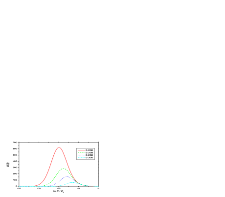
Figure 1: Fig. 1. The density of states $D(E)$ in units of $n_{L}/\pi E_{0}$ as a function of $\ln E/E_{0}$ for different values of impurity concentration $f$.

5. Conclusion.

In conclusion, we evaluated the density of states of a two-dimensional electron gas in the presence of the strong magnetic field and impurities. The fact that impurities are situated at different distances from two-dimensional electron gas leads to the dramatic change of the density of states in the case of small impurity concentration compared to the case when all impurities are situated at the same distance from the 2DEG.

Using the exact result of Ref. [7] we obtained the density of states in the whole energy range for the case of the wave function with the asymptotic behavior (4). The density of states vanishes at the position of the unperturbed Landau level and has a maximum at an exponentially small energy (9). The major part of the states are localized by single impurities in accordance with findings of Ref. [9].

The functional form of the result will be different for asymptotic behavior of $\varphi(z)$ differing from the simple exponential decay (4). However, the qualitative structure of the density of states is supposed to be preserved.

We acknowledge useful discussions with M.V. Feigelman, S.V. Iordansky, A.S. Iosselevich, D. Lyubshin, and P.M. Ostrovsky. We are grateful to A.M. Dyugaev, P.D. Grigoriev and Yu.N. Ovchinnikov for bringing their paper to us prior to publication. We thank Forschungszentrum Jülich (Landau Scholarship) (I. S. B.), Dynasty Foundation, ICFPM, RFBR under grant 01-02-17759, and Russian Ministry of Science (M. A. S.) for financial support.

References

- [1] For a review, see T. Ando, A.B. Fowler, and F. Stern, Rev. Mod. Phys. 54, 437 (1982)
- [2] For a review, see The quantum Hall effect, ed. by R.E. Prange and S.M. Girvin (Springer-Verlag, Berlin, 1987).
- [3] I.V. Kukushkin, S.V. Meshkov, and V.B. Timofeev, Usp. Fiz. Nauk 155, 219 (1988)
- [4] T. Ando and Y. Uemura, J. Phys. Soc. Japan 36, 959 (1974); ibid 36, 1521 (1974); T. Ando, ibid 37, 1233 (1974)
- [5] K.B. Efetov and V.G. Marikhin, Phys. Rev. B 40, 12126 (1989)
- [6] F. Wegner, Z. Phys. B 51, 279 (1983)
- [7] E. Brezin, D.J. Gross, and C. Itzykson, Nucl. Phys. B 235, 24 (1984)
- [8] E.M. Baskin, L.N. Magarill, and M.V. Entin, Zh. Eksp. Teor. Fiz. 75, 723 (1978)[Sov. Phys. JETP , 48, 365 (1978)]
- [9] A.M. Dyugaev, P.D. Grigoriev, and Yu.N. Ovchinnikov, cond-mat/0307064.
- [10] L.B. Ioffe and A.I. Larkin, Zh. Eksp. Teor. Fiz. 81, 1048 (1981) [Sov. Phys. JETP , 54, 556 (1981)]
- [11] I. Affleck, J. Phys. C 17, 279 (1984)