On size and growth of business firms

Abstract

We study size and growth distributions of products and business firms in the context of a given industry. Firm size growth is analyzed in terms of two basic mechanisms, i.e. the increase of the number of new elementary business units and their size growth. We find a power-law relationship between size and the variance of growth rates for both firms and products, with an exponent between -0.17 and -0.15, with a remarkable stability upon aggregation. We then introduce a simple and general model of proportional growth for both the number of firm independent constituent units and their size, which conveys a good representation of the empirical evidences. This general and plausible generative process can account for the observed scaling in a wide variety of economic and industrial systems. Our findings contribute to shed light on the mechanisms that sustain economic growth in terms of the relationships between the size of economic entities and the number and size distribution of their elementary components.

1 Introduction

This work is rooted in the “old” stochastic tradition of the analysis of economic and industrial growth [1]. We elaborate on some recent contributions [2, 3, 4], focusing on the shape and width of growth rates distributions. Size and growth distributions for firms and products are analyzed in the context of the worldwide pharmaceutical industry, over a period of ten years. We consider the entire population of firms and products, as well as entry and exit of firms and products. In accordance with [2] and [3], we find the distribution of growth rates to be non-Gaussian with heavy tails. Moreover, for both products and firms, the width of the growth distribution scales as a power law of size, with a scaling exponent $\beta$ between -0.17 and -0.15, which is remarkably stable upon aggregation. We introduce a general framework to account for the observed regularities, drawing some general implications on the mechanisms which sustain economic and industrial growth. We show that [1, 5] can be extended to account for the shape of size and growth distributions, as well as for scaling relationships at different levels of aggregation. Products are considered as business opportunities which are captured and lost by firms, and then grow in size. Both the capture and loss of business opportunities are modelled as an instantiation of the Law of Proportionate Effect applied to elementary business units. Then, each elementary unit is assumed to grow in size according to a process of proportional growth based on random multiplicative dynamics, with shocks independently and randomly drawn from a lognormal distribution. This simple and general framework accounts for the most salient features of size and growth distributions at different levels of aggregation.

2 Empirical findings

Data used in this work are drawn from the Pharmaceutical Industry Database (PHID) at CERM/EPRIS. PHID records quarterly sales figures of 48,819 pharmaceutical products commercialized by 3,919 companies in the European Union and North America from September 1991 to June 2001 (values are in Sterling at constant 2001 exchange rates). Information is available on entry and exit of firms and products over time, and the entire size distribution is covered.

$S_{m,i,j}(t)$ denotes sale figures at time $t$ for the market ($m$), at the level of each firm ($i$), and at the product level ($j$), respectively:

$$S_{m}(t)={\textstyle\sum\limits_{i=1}^{M}}S_{i}(t)=\overset{M}{\underset{i=1}{{\textstyle\sum}}}\underset{j=1}{\overset{N_{i}}{{\textstyle\sum}}}S_{ij}(t)$$

where $M$ is the total number of firms active at time $t$ and $N_{i}$ is the number of products of the $i$-th firm. Throughout the paper we focus on firm internal growth. We study the logarithm of growth rates:

$$g_{m,i,j}(t)=\log(G_{m,i,j}(t))=\log\left(\frac{S_{m,i,j}(t)}{S_{m,i,j}(t-1)}\right)=s_{m,i,j}(t)-s_{m,i,j}(t).$$

Market size has more than doubled from 61.500 to 159.000 £M from 1991 to 2001 (+154%). The growth of the market was sustained by the entry of new products. The number of products has increased linearly from about 25,000 to more than 35,000, while the number of firms has remained almost constant around 2,000. Both the mean and the standard deviation of the number of products by firm have increased linearly in time, from 12.5 to about 17 and from 44 to about 54, respectively. The rapid market expansion of the market notwithstanding, the first two moments of the logarithm of size and growth distributions have been almost stationary, apart from a marked seasonality (see Fig. 1.b-c). Both product and firm growth distributions are non-Gaussian and leptokurtotic (Fig. 2a).Size distributions for both products and firms are consistent with a log-normal fit (Fig. 2b) apart from a pronounced Pareto upper tail $1/S$.

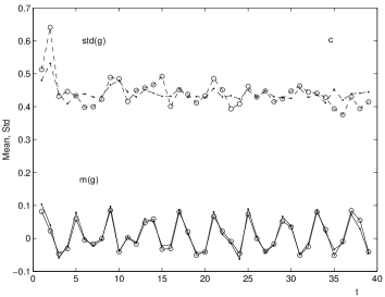
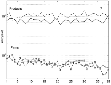
Figure 1: Descriptive statistics. Fig. 1.a - Overall market size (dots) and market size without entry of new products (circles). Fig. 1.b - Product (dots) and firm (circles) size; mean and standard deviation. Fig. 1.c - Product (dots) and firm (circles) growth; mean and standard deviation. Fig. 1.d - Entry (full line) and exit (dashed line) patterns of products (dots) and firms (circles). All values are in logarithmic scale.

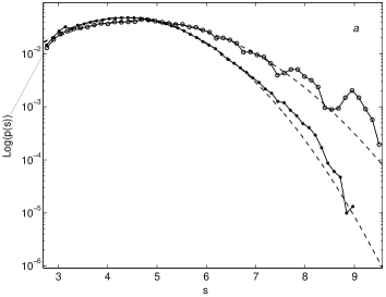
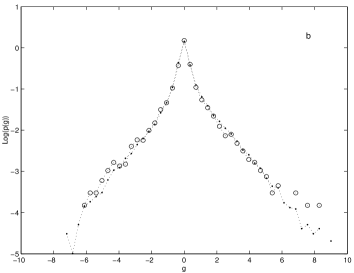
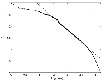
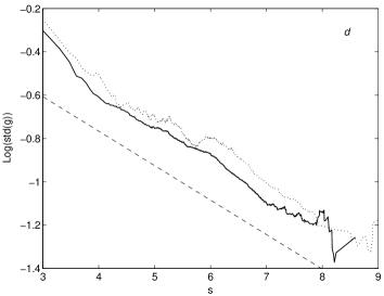
Figure 2: Probability distributions and the size-variance relationships (log10-log10 plots). Fig. 2.a - Size distributions, products (dots) and firms (circles). Gaussian fit: products (.048, 4.34, 1.59); firms (.043, 4.63, 1.97). Fig. 2.b - Product (dots) and firm (circles) growth distributions. Fig. 2.c - Zipf plot of the number of products by firm in 2001. Pareto fit: -1.06 ($\pm.05$). Fig. 2.d - Size-variance relationship for products (full line) and firms (dotted line). Linear slope coefficients are -.167 ($\pm.005)$ for firms and -.156 ($\pm.012)$ for products ($-.16$ reference line.)

Since a few seminal contributions [6, 7, 8], it is well known that the standard deviation of firm growth rates tends to decrease with firm size less rapidly than the square root of size. Recently, [2] and [3] have provided a robust characterization to this stylized fact by fitting a power law relationship of the form $std(g)=cS^{\beta}$ and estimating the power coefficient $\beta$ in the range $-.15$ to $-.21.$ Fig. 2.d shows similar results for both pharmaceutical products and companies ($\beta\cong-.16).$ As in [3], this departure from the prediction of the Law of Large Numbers cannot be interpreted as the effect of some form of correlation of growth rates across constituent units at the level of each firm. In fact, the mean cross-correlation of products at the firm level is weak ($.07),$ and its effect is too small to account for the flatness of the scaling relationship. Fig. 2.c. reports the Zipf’s plot of the relationship between $Log(N_{i})$ and the logarithm of the rank of companies in terms of number of subunits. The distribution of the number of products can be approximated by a Pareto distribution with a slope coefficient of $-1.06$ with a departure in the tails (first 20 companies and small firms with less than 10 products).

As for growth rates, some departures from a pure Gibrat process can be detected. First, the stationarity of the variance substantiates a first deviation from a Gibrat growth process, which predicts a linear increase of the variance with time. Second, the standard deviation of the growth rates does not decrease according to $\frac{1}{\sqrt{S}}$. Third, the growth distributions are non-Gaussian and leptokurtotic.

3 Scaling properties and proportional growth

Firms grow through the launch of new products and the growth in size of existing products. This two-way mechanism is essential to characterize the firm growth process, which is assumed here to be the outcome of the law of proportional effect applied on sizes and number of opportunities. In this section, we investigate how these two mechanisms affect the shape of the growth distributions at different levels of aggregation and the scaling relationship.

Like in [5], each distinguishable arrangement of products at the firm level is assumed to have an equal probability of occurrence. Assignment or loss of business opportunities to firms is modelled by randomly selecting firm $i$ proportionally to the number of its products $N_{i}$. Each time a firm is selected a new product is given to that firm. In this way, the number of products assigned represents the total time of the simulation. Then, new firms are added at rate $\alpha$, and old products are removed every $1/\delta$ new product assignments. In line with our empirical findings, this model leads to a Pareto distribution of the number of constituent business units [5]. Once captured, each elementary unit is assumed to grow in size following a geometric process which in logs reads $ds_{t}=adt+bdW_{t}$. We set $a=0$ and $b$ small, sampling the initial size $S_{0}$ of new products from a sum of lognormal distributions with mean and standard deviation equal to the empirically observed values $(3.48$, $2.27)$. The result of the simulation is plotted in Fig. 3 together with the empirical growth distribution for products and firms. It is obtained by assigning $25,000$ products to $2,000$ firms. Then, further $10,000$ products are added, with $\alpha=0.01$ and $\delta=0.05$.

Figure 3: Left: Dependence of $\beta$ in the scaling relation $std(g)=S^{\beta}$ against the coefficient $\sigma$ of the underlying size distribution. Right: Growth distributions, empirical (dots for products, circles for firms) and simulative results (solid line).

The logarithm of firm size $S_{i}$ at time $t$ is equal to the logarithm of the sum of the sizes of its constituent components ($s_{i}=\log\left(\sum_{j}S_{j}\right)$). As we have shown in Section 2, both product and firm sizes $S$ are approximately distributed as a log-normal distribution with an upper tail which decays as a power law. The sum of lognormally distributed random variables does not have a close form, while several possible approximations have been proposed for the first two moments, which involve series evaluations. These estimates are all based on the approximation that a sum of lognormals is still a lognormal distribution [9], stable upon aggregation. In fact, a log-normal distribution $p(S)$ with parameters ($\mu,\sigma$) behaves as a power law between $S^{-1}$ and $S^{-2}$ for a wide range of its support $S_{0}<S<S_{0}e^{2\sigma^{2}}$, where $S_{0}$ is a characteristic scale corresponding to the median [10]. Since a decay similar to power-law is present for a large part of the upper tail, the central limit theorem does not work effectively. This argument explains the stability of size distributions upon aggregation. In particular, simple numerical simulations show that $\log\left(\sum_{j}S_{j}\right)$ depicts a Pareto $1/S$ tail, in line with the empirical distributions.

For a fixed number of products, numerical simulations show that $p(g)$ is to a good approximation distributed as a Laplace. In fact, because logarithms of sum of lognormal distributions in $S$ tend to an exponential in the upper tail for $\log(S)$, the difference is distributed as a Laplace on the tails. The scaling relationship is $std(g)=S^{\beta}$, with $\beta$ dependent on the standard deviation of the underlying size distribution. The coefficient $\beta$ goes from $-0.5$ for $\sigma$ very small to zero for a large $\sigma$. In the parameter range of our empirical data, $\beta$ is between $-0.1$ and $-0.2$ for a variance of the underlying size distribution that spans over three orders of magnitude. This process of size growth by itself has a small variance and influences the observed growths only in the central part of the distribution. Moreover, although the variance of $s$ for this process tends to increase linearly in time, we find its magnitude to be very small, accounting for the observed stationarity of the standard deviation of the log-size $s$ in the spanned time period. The shape of the empirical growth distributions is mostly due to the growth in number of products and to the distribution of the aggregation process in $N_{i}$ which produces the result plotted in Fig 3.

4 Conclusions

This paper shows that the framework originally developed by H. A. Simon and Y. Ijiri can be extended to account for some universal features in economic and industrial growth, which have been detected across different domains following [2]. Our work aims at providing a simplified framework to investigate the mechanisms that sustain processes of economic growth, in terms of the static and dynamic relationships between the size of economic entities and the number and size distribution of their elementary constituent components. It shows that two multiplicative growth processes in number of opportunities and size are able to reproduce most of the salient aspects of the empirical growth process. In particular, the model predicts that the scaling relation is stable for a wide range of variances of the underlying size distribution, and the growth process is stable upon aggregation. Further research is needed to articulate the assumptions of the outlined framework in different regimes of growth, in the direction of building parsimonious and realistic representations of economic and industrial growth.

References

- [1] Y. Ijiri, H. Simon, Skew Distributions and the Size of Business Firms, North Holland, 1977.
- [2] M. H. E. Stanley, L. A. N. Amaral, S. V. Buldyrev, S. Havlin, H. Leschhorn, P. Maass, M. A. Salinger, H. E. Stanley, Nature 379 (1996) 804.
- [3] J. Sutton, Physica A 312 (2002) 577.
- [4] X. Gabaix, Power laws and the origin of the business cycle, preprint (2002).
- [5] Y. Ijiri, H. Simon, Proc. Nat. Acad. Sci. 72 (1975) 1654.
- [6] S. Hymer, P. Pashigian, J. Pol. Ec. 70 (6) (1962) 556.
- [7] E. Mansfield, Am. Ec. Rev. 48 (1962) 607.
- [8] H. Simon, J. Pol. Ec. 72 (1) (1964) 81.
- [9] S. C. Schwartz, Y. Yeh, The Bell System Technical Journal 61 (7) (1982) Sept.
- [10] D. Sornette, Critical Phenomena in Natural Sciences, Springer, 2000.