Rare Events and Scale–Invariant Dynamics of Perturbations in Delayed Dynamical Systems

Abstract

We study the dynamics of perturbations in time delayed dynamical systems. Using a suitable space-time coordinate transformation, we find that the time evolution of the linearized perturbations (Lyapunov vector) can be described by the linear Zhang surface growth model [Y.-C. Zhang, J. Phys. France 51, 2129 (1990)], which is known to describe surface roughening driven by power-law distributed noise. As a consequence, Lyapunov vector dynamics is dominated by rare random events that lead to non-Gaussian fluctuations and multiscaling properties.

Deterministic chaos is an ubiquitous feature of nonlinear systems and much is understood about its dynamical properties in low-dimensional systems. Lyapunov exponents, measuring the separation of initially nearby trajectories, have demonstrated to be helpful in characterizing chaotic motion in systems with a few degrees of freedom schuster . In the case of spatially extended nonlinear systems, a straightforward generalization leads to the concept of Lyapunov exponent density or spectrum, but the problem here is more complex and one must take into account propagation and diffusion phenomena that complicate much the problem bohr .

Pikovsky et al. pik1 ; pik2 have recently shown that the Lyapunov vector, which contains the spatial dependence of the diverging growth rate of the linearized perturbations, can be described as a nonequilibrium growing interface. Moreover, they have reported that in many cases, as for instance in coupled-map lattices, Lyapunov vector growth is consistent with that of the well-known Kardar-Parisi-Zhang (KPZ) equation kpz of surface growth. In the case of systems with a conservation law, one has to be more cautious since KPZ scaling might be not satisfied, e.g., for the Hamiltonian lattices studied in Ref. pik3 . An interesting question that naturally arises is whether the dynamics of perturbations in extended systems could be divided in a few universality classes of growth according to the existence of symmetries and/or conservation laws, as occurs in nonequilibrium surface growth baraba&stanley .

In this Letter we study Delayed Dynamical Systems (DDSs), which are formally infinite dimensional dynamical systems and show many aspects of space-time chaos. DDSs appear in a number of biological and physical situations, e.g., regulation of blood cells production mg , lasers with delayed feedback ikeda ; arecchi1 , etc. In recent years, DDSs have attracted a renewed interest as they have been proposed as candidates for secure communication systems based upon semiconductor lasers with time-delayed optical feedback roy ; goedgebuer .

Our aim in this Letter is to show that the dynamics of the Lyapunov vector in DDSs can be generically described by a stochastic surface growth equation in which rare fluctuations play a most important role. We argue that the growth model belongs to the universality class of the linear Zhang model zhang1 ; krug ; baraba ; lopez ; baraba&stanley . This is in contrast with other spatially extended dynamical systems that in general lead to KPZ-like growth of the amplitude perturbations pik1 ; pik2 . Our results clearly show that, although DDSs are usually interpreted as extended dynamical systems with hyper-chaotic behavior, they exhibit distinctive features, including multiscaling and intermittent driving fluctuations, not shared with other space-time chaos systems.

A broad class of systems with delayed feedback are given by differential-delay equations such as

$$\dot{y}={{dy}\over{dt}}={\cal F}(y,y_{\tau}),$$ (1)

where $y_{\tau}=y(t-\tau)$ is the delayed variable and $\tau$ is time delay. A canonical example is the Mackey-Glass model mg (see below), for which it has been shown that the number of positive Lyapunov exponents grows linearly with the time delay farmer .

Generic surface growth model for DDSs.–

Any DDS can be interpreted as a spatially extended system by introducing a simple transformation, $t=x+\theta\,\tau$, where $x\in[0,\tau]$ is the space variable, while $\theta\in\mathbb{N}$ is a discrete time variable arecchi2 . This is a powerful representation in which the formation and propagation of structures, defects and spatiotemporal intermittency can be more easily identified arecchi2 . Note that the time delay $\tau$ becomes the system size in such a way that the time dependence with the delayed variable is transformed into a short-range interaction within the horizontal space coordinate $x$ in the space-time representation.

The dynamics of propagation of localized disturbances, i.e. the Lyapunov vector, can be obtained by linearizing (1) which, after the transformation to space-time representation, becomes politispace

$$\nabla\phi(x,\theta)=u\,\phi(x,\theta)+v\,\phi(x,\theta-1),$$ (2)

where $\nabla=\partial_{x}$, $\phi(x,\theta)=\delta y(x,\theta)$ is the Lyapunov vector, and $u={\partial\cal F}/{\partial y}$ and $v={\partial\cal F}/{\partial y_{\tau}}$.

Following Pikovsky et. al. pik1 ; pik2 , we can map this equation into a surface growth model by introducing the surface height as $h(x,\theta)=\log|\phi(x,\theta)|$. Then, after defining $\partial_{\theta}\phi(x,\theta)=\phi(x,\theta+1)-\phi(x,\theta)$, one easily obtains the corresponding growth equation for the surface. We finally arrive to the equation,

$$\partial_{\theta}h=-(1/v)\,\nabla h+(u/v)+1,$$ (3)

where $\nabla h=\partial_{x}h$ and the boundary conditions $h(\tau,\theta)=h(0,\theta+1)$.

In the following we restrict ourselves to the most studied case of DDSs in the chaotic regime, in which $u={\rm const}$ and $v$ is a nonlinear function (see Eq.(6) below), so that $1/v$ will play the role of a noise source. As we shall see below, probability distribution and correlation of this noisy term will turn out to be essential for understanding the behavior of the growth equation. Note that, if $P_{v}(v)$ is the probability density function (PDF) of $v$, the corresponding PDF of $\zeta=1/v$ is given by $P_{\zeta}(\zeta)=|\zeta|^{-2}P_{v}(1/\zeta)$. Therefore, if $P_{v}$ behaves as $P_{v}(v)\sim|v|^{\nu}$ when $v\to 0$, we have that the PDF of $\zeta$ is then given by $P_{\zeta}(\zeta)\sim|\zeta|^{-(2+\nu)}$ for large $|\zeta|$ (conversely for small $|v|$). This power-law decay distribution of the noise is very remarkable and leads to a dynamics dominated by rare fluctuations. The occurrence of large events of amplitude $|\zeta|\gg 1$ has a small but non-negligible probability (they take place whenever the function $v$ gets close to zero). As we will show below, these rare fluctuations drive the system towards a stationary state that displays multiscaling properties. Anticipating part of our numerical results, in Figure 1 we plot the PDF of the chaotic function $\zeta$ for the Mackey-Glass model, which, as expected from our theoretical arguments, decays as a power-law $P_{\zeta}(\zeta)\sim|\zeta|^{-2.42}$.

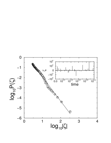
Figure 1: Numerical simulation of the Mackey-Glass model. Inset shows a typical realization of the chaotic function $\zeta=1/v$ in time, in which the pronounced non-Gaussian fluctuations are already visible. Main panel shows the power-law behavior of the probability density of $\zeta$ obtained for time delays $\tau=500$ ($\circ$) and $\tau=2000$ ($\Box$). The line is a least-mean square fit to the data with slope $-2.42$.

The important fact that the surface growth equation that describes the propagation of disturbances in DDSs, Eq.(3), is dominated by rare fluctuations strongly suggests that the universality class of growth to which the surface must belong is the well-know linear Zhang model:

$${\partial_{\theta}h}=D\,\nabla^{2}h+f_{0}+\eta(x,\theta),$$ (4)

which is the representative model of the universality class of linear surface growth in the presence of power-law noise zhang1 ; krug ; baraba ; lopez ; baraba&stanley . This model is expected to describe the dynamics of the Lyapunov vector in DDSs for large enough systems (i.e. long enough delay times). KPZ-like nonlinearities such as $(\nabla h)^{2}$ are not expected to appear in the effective surface growth equation, since Eq.(3) is statistically invariant under the $h\to-h$ transformation and this symmetry must be preserved. Moreover, for the class of systems we are interested in this Letter, $u(x,\theta)={\rm const}$ and a simple scaling argument shows that the additive noise in Eq.(4) must be $\eta\propto\sqrt{\zeta}$. So, we expect the effective noise term $\eta$ in Eq.(4) to be distributed according to a power-law, $P(\eta)\sim\eta^{-(1+\mu)}$, where the noise index is $\mu=2\,(1+\nu)$. Further justification that Eq.(3) is in the universality class of the linear Zhang model can be given as follows. By making use of standard stochastic functional techniques, like Novikov’s theorem ojalvo&sancho ; novikov , spatial average of the stochastic drift term $\zeta\,\nabla h$ can be calculated explicitely for the simpler case of Gaussian noise to obtain $D\nabla^{2}h+b\nabla h$, where the constants $D$ and $b$ are related to space-time noise correlator integrals (see for instance Ref. ojalvo&sancho ). In the case of noise with zero mean value and an even spatially homogeneous correlation function $\langle\eta(x,t)\eta(x^{\prime},t^{\prime})\rangle$ one obtains a vanishing drift term $b=0$.

In the context of surface kinetic roughening, Eq.(4) corresponds to the well-known linear Zhang model zhang1 ; krug ; baraba ; lopez ; baraba&stanley that describes the surface height dynamics in the presence of an uncorrelated power-law distributed noise source. In the following, we shall briefly review the scaling properties of this growth model. The height $h(x,t)$ exhibits scale-invariant properties characterized by the scaling behavior of the surface fluctuations as measured by the global width, $W(L,t)=\langle\overline{[h(x,t)-\overline{h(x,t)}]^{2}}\rangle^{1/2}$, where the average is calculated over all $x$ in a system of horizontal size $L$ (overline) and noise (brackets). Space and time scale-invariance leads to the scaling behavior of the width,

$$W(L,t)\sim\left\{\begin{array}[]{lcl}t^{\beta}&{\rm if}&t\ll L^{z}\\ L^{\alpha}&{\rm if}&t\gg L^{z}\end{array}\right..$$ (5)

The critical exponents $\alpha$ and $\beta$ are the roughness and growth exponent, respectively, and characterize the global scaling behavior of the surface height. The dynamic exponent $z$ is related with the horizontal extent of the correlation length $l_{\times}\sim t^{1/z}$ and fulfills the usual relation $z=\alpha/\beta$. A simple mean-field approximation krug ; baraba&stanley provides estimates of the scaling exponents that depend on the index $\mu$ characterizing the power-law decay of the noise as follows. The dynamics is diffusive ($z=2$) for any value of $\mu$. However, the global roughness exponent depends on the noise index, $\alpha=(3-\mu)/\mu$ for $\mu\leq 2$, when the fluctuations are dominated by rare events, and $\alpha=1/2$ for $\mu\geq 2$, where the noise distribution tail becomes irrelevant and standard Gaussian behavior is recovered krug ; baraba&stanley . Another interesting aspect of roughening dominated by power-law noise is multiscaling –namely, higher moments of the height-height correlation function do not scale with the same exponents– which indicates that the height distribution is far from Gaussian and dominated by rare fluctuations of the noise. In particular, multiscaling behavior in the linear Zhang model occurs for noise indexes in the range $1<\mu<3$ lopez2 . This behavior is analogous to that observed in the velocity fluctuations of turbulent fluids turbulence as well as in some solid-on-solid models of epitaxial growth krug-mbe ; baraba&stanley . Multiscaling properties can be proven by calculating the $q$th order height-height correlation function $G_{q}(x,t)=\langle\overline{|h(x_{0}+x,t)-h(x_{0},t)|^{q}}\rangle^{1/q}$, which scales as $G_{q}(x,t)\sim t^{\beta_{q}}$ for short times and saturates, $G_{q}(x)\sim x^{\alpha_{q}}$, for long enough time zhang1 ; krug ; baraba ; baraba&stanley . Exponents $\alpha_{q}$ and $\beta_{q}$ that depend on the index $q$ are the characteristic fingerprint of multiscaling behavior.

Numerical results.–

We have carried out extensive numerical simulations of several chaotic delayed systems in order to compare with our theoretical findings. We have studied the well-known class of systems

$$\dot{y}=-a\,y+F(y_{\tau}),$$ (6)

which have been used in the past for a variety of applications ranging from biology mg to lasers with feedback ikeda ; roy ; goedgebuer . For the particular choices $F(\rho)=b\,\rho/(1+\rho^{10})$, $F(\rho)=b\,\sin(\rho-\rho_{0})$ and $F(\rho)=b\,\sin^{2}(\rho-\rho_{0})$, which correspond to the Mackey-Glass mg , Ikeda ikeda , and the delayed feedback model for secure optical communications goedgebuer , respectively. For this class of systems, the function $u$ is constant, $u=-a$, and the additive noise in Eq.(4) is $\eta(x,\theta)\propto\sqrt{1/v}$, where the nonlinear function $v=dF/d\rho$. In all our numerical simulations we have used the Adams-Bashforth-Moulton predictor-corrector scheme nr . From the numerical solution of the corresponding equation for the evolution of the perturbations of the leading Lyapunov exponent, Eq.(2), we have constructed the surface $h(x,\theta)=\log|\phi(x,\theta)|$ following the procedure above discussed to get the space-time mapping. After that, the scaling properties of the resulting surface have been studied. For the sake of brevity we focus the discussion of numerical results on the Mackey-Glass model, but similar results were found for the other two systems studied. The parameters $a=0.1$ and $b=0.2$ are used in all the results we are presenting here, and simulation with a time delay varying from ten to a few thousand time units have been carried out. The region of interest here corresponds to delays $\tau\gg 17$ for which the Mackey-Glass model is known to be hyper-chaotic farmer .

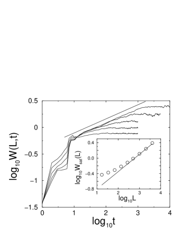
Figure 2: Time evolution of the global surface width in the Mackey-Glass model for different system sizes $L=272,5\times 10^{2},10^{3},2\times 10^{3},4\times 10^{3}$ (time delays). The straight line is a guide to the eye and has a slope $\beta=0.25$. Inset shows a log-log plot of the stationary $W_{sat}(L)$ vs. $L$ (flat late regime of the main panel data). The line is a guide to the eye with slope $\alpha=0.5$.

In Figure 1 (inset) we show a typical run of the simulation for the Mackey-Glass system with a time delay $\tau=500$ . The intermittent behavior of $\zeta$ is already apparent in the form of large peaks in the inset plot. We recorded the values taken by $v$ and collected statistics from long runs in order to obtain the PDF of the noise $\zeta=1/v$. In Fig. 1 we show our results for two instances of the time delay $\tau=500,\,2000$. We obtain a power-law distribution $P_{\zeta}(\zeta)\sim|\zeta|^{-2.42}$ that is independent of the time delay used and corresponds to an exponent $\nu=0.42\pm 0.02$. The power spectrum of $\zeta$ (not shown) is flat indicating that $\zeta$ lacks long-range temporal correlations. We then expect the noise in the effective surface growth model (4) to be power-law distributed with $\mu=2\,(1+\nu)=2.84\pm 0.04$. This value of the noise index $\mu>2$ implies, according to the mean-field prediction for the linear Zhang model, that the roughness and growth exponent should be $\alpha=1/2$ and $\beta=1/4$, respectively. Very interestingly, it also implies that one should observe multiscaling behavior, since $\mu\in(1,3]$.

Figure 3: Multiscaling behavior of the stationary $q$th correlation function of the surface in the Mackey-Glass model (dashed lines) with a delay $L=10^{3}$ for $q=1,2,3,4,5$ (from bottom to top). Linear mean least-square fits (solid lines) give an estimation of the multiscaling roughness exponents as $\alpha_{1}=0.786(6)$, $\alpha_{2}=0.496(2)$, $\alpha_{3}=0.328(1)$, $\alpha_{4}=0.257(1)$, $\alpha_{5}=0.210(1)$.

In Figure 2 we plot the time behavior of the surface width for different system sizes $L$ (i.e. time delays $\tau$) for the Mackey-Glass system. From that figure we obtain an estimation of the growth exponent $\beta=0.25\pm 0.03$ in the intermediate times regime, before a stationary state is reached. The scaling regime appears after an earlier short transient regime (of about one decade), and becomes longer for larger system sizes. For the largest system we used $L=4\times 10^{3}$ the scaling regime lasts for about two decades. After saturation, which occurs at times $t_{sat}\sim L^{z}$, the surface height becomes scale-invariant and the width grows as $W(t\gg t_{sat},L)\sim L^{\alpha}$, with a roughness exponent $\alpha=0.50\pm 0.05$. From the inset of Fig. 2, it becomes clear that our estimation of the roughness exponent fits better in the limit of large system size, showing that long delays are required to reach the true scaling regime. These exponent values agree with the theoretical values predicted for the Zhang model for a noise index $\mu=2.84>2$.

Finally, we have also studied numerically the existence of multiscaling phenomena. In Figure 3, we plot the $q$th height-height correlation function for the Mackey-Glass system with time delay $\tau=10^{3}$. Multiscaling behavior is obtained for any time delay larger than $\tau\approx 17$, which is the lower bound for chaos to appear in the system. However, multiscaling becomes clearer in larger systems (longer time delays), since the multiscaling region has a larger expand. As predicted by our theoretical arguments, multiscaling behavior is to be expected whenever $\mu<3$. Crossover to self-affine scaling is observed on large scales as generically expected for surface roughening driven by rare events (see baraba&stanley ; baraba for details).

Conclusions.–

Symmetry and scaling considerations have led us to conclude that the linear Zhang model for surface roughening driven by power-law noise describes the dynamics of the Lyapunov vector for long enough time delays. We then argue that DDSs generically display multiscaling of fluctuations due to the power-law nature of the driving noise.

The interpretation of DDSs as spatial systems has also been used in practical applications, in particular for the analysis of experimental data of $CO_{2}$ lasers with optical feedback arecchi2 . The technique allowed to identify many spacelike properties in experiments, including defects formation, transitions between weak and fully developed turbulence, etc. However, we have established a precise difference between high-dimensional chaos in delayed systems and in truly extended systems (like coupled-map lattices, partial differential equations, etc). Our results also suggest that different high-dimensional chaotic systems could be divided into a few universality classes based upon basic symmetries and conservation laws, akin to what occurs in scale-invariant surface growth.

- (1) H. G. Schuster, Deterministic Chaos, An Introduction, VCH-Verlag, Meinheim, (1988).
- (2) T. Bohr, et al., Dynamical Systems Approach to Turbulence, Cambridge U. P. Cambridge (1998).
- (3) A. Pikovsky and J. Kurths, Phys. Rev. E 49, 898 (1994).
- (4) A. Pikovsky and A. Politi, Nonlinearity 11, 1049 (1998).
- (5) M. Kardar, G. Parisi, and Y. C. Zhang, Phys. Rev. Lett. 56, 889 (1986).
- (6) A. Pikovsky and A. Politi, Phys. Rev. E 63, 036207 (2001).
- (7) A. -L. Barabási and H. E. Stanley, Fractal Concepts in Surface Growth, Cambridge U. P., Cambridge, (1995).
- (8) M. C. Mackey and L. Glass, Science 197, 287 (1977).
- (9) K. Ikeda, Opt. Commun. 30, 257 (1979).
- (10) F. T. Arecchi, W. Gadomski and R. Meucci, Phys. Rev. A 34, 1617 (1986).
- (11) G. D. van Wiggeren and R. Roy, Science 279, 1198 (1998).
- (12) V. S. Udaltsov et al., Phys. Rev. Lett. 86, 1892 (2001).
- (13) Y. -C. Zhang, J. Phys. France 51, 2129 (1990).
- (14) J. Krug, J. Phys. I 1, 9 (1992).
- (15) A. -L. Barabási, et al., Phys. Rev. A 45, R6951 (1992).
- (16) J. M. López, Mod. Phys. Lett. B 13, 423 (1999).
- (17) J. D. Farmer, Physica D 4, 366 (1982).
- (18) F. T. Arecchi et al., Phys. Rev. A 45, R4225 (1992); G. Giacomelli et al., Phys. Rev. Lett. 73, 1099 (1994).
- (19) G. Giacomelli and A. Politi, Phys. Rev. Lett. 76, 2686 (1996).
- (20) J. García–Ojalvo and J. M. Sancho, Noise in Spatially Extended Systems, Springer-Verlag, New York z (1999).
- (21) E. A. Novikov, Sov. Phys. JETP 20, 1290 (1965).
- (22) J. M. López (unpublished).
- (23) U. Frisch, Turbulence, Cambridge U. P. Cambridge (1995).
- (24) J. Krug, Phys. Rev. Lett. 72, 2907 (1994).
- (25) W. H. Press et al., Numerical Recipes, Cambridge U. P. Cambridge (1992).