Fluctuation and localization of acoustic waves in bubbly water

Abstract

Here the fluctuation properties of acoustic localization in bubbly water is explored. We show that the strong localization can occur in such a system for a certain frequency range and sufficient filling fractions of air-bubbles. Two fluctuating quantities are considered, that is, the fluctuation of transmission and the fluctuation of the phase of acoustic wave fields. When localization occurs, these fluctuations tend to vanish, a feature able to uniquely identify the phenomenon of wave localization.

Among many unsolved problems in condensed matter physicsRama , the phenomenon of Anderson localization is perhaps most intriguing. The concept of localization was first proposed about 50 years ago for possible disorder-induced metal-insulator transitionAnderson . That is, the electronic mobility in a conducting solid could completely come to a halt when the solid is implanted with a sufficient amount of randomness or impurities, in the absence of the electron-electron interaction. As a result, the electrons tend to stay around the initial site of release, i. e. localized, and the envelop of their wave functions decays exponentially from this site Lee . The physical mechanism behind is suggested to be the multiple scattering of electronic waves by the disorders.

Ever since the inception of this concept, considerable efforts have been devoted to observing localization or phenomena possibly related to localization, as reviewed in, for instance, Ref. Lee ; Thouless ; loc . By analogy with electronic waves, the concept of localization has also been extended to classical systems ranging from acoustic and electromagnetic waves to seismological waves in randomly scattering media, yielding a vast body of literature (Refer to the reviews and textbooks Refs. John ; Sheng ; Lagen ; Seis ). In spite of these efforts, the phenomenon of localization has remained as a conceptual conjecture rather than a reality that has been observed conclusively.

The difficulty in observing electronic localization may be obvious. In actual measurements, the Coulomb interaction between electrons is hard to be excluded. With this in mind, it has been suggested that localization might be easier to observe for classical waves as wave-wave interactions are often negligible in these systems. However, classical wave localization may yet suffer from effects of absorption, leading to uncertainties in data interpretation. Indeed, up to date, a definite experimental evidence of localization is still lacking. Significant debates on reported experimental results remain McCall ; Meade ; Wiersma . How to unambiguously isolate localization effects from other effects therefore stays on the task list of top priority, and poses an compelling issue to our concern.

In this Letter, we wish to continue previous efforts in exploring acoustic localization in water having many air-filled bubbles, i. e. bubbly water Alberto ; APL . We attempt to identify some unique features associated with localization. In particular, we will study the behavior of the phase of the acoustic wave fields in bubbly water. The fluctuation of the phase and the acoustic transmission will be studied. The method is based upon the standard multiple scattering theory which has been detailed in Ken .

Consider the acoustic emission from a bubble cloud in water. For simplicity, the shape of the cloud is taken as spherical. Such a model eliminates irrelevant edge effects, and is useful to separate phenomena pertinent to discussion. Total $N$ bubbles of the same radius $a$ are randomly distributed within the cloud. The volume fraction, the space occupied by bubbles per unit volume, is taken as $\beta$; thus the numerical density of bubbles is $n=3\beta/(4\pi a^{3})$, and the radius of the bubble cloud is $R=(N/\beta)^{1/3}a$. A monochromatic acoustic source is located at the center of the cloud. Adaptation of such a model for other geometries and situations is straightforward. The wave transmitted from the source propagates through the bubble layer, where multiple scattering incurs, and then it reaches a receiver located at some distance from the cloud. The multiple scattering in the bubbly layer is described by a set of self-consistent equations. The energy transmission and the acoustic wave field can be solved numerically in a rigorous fashion Alberto ; Ken .

Denoting the total acoustic wave at a spatial point as $p(\vec{r})$, which includes the contributions from the wave directed from the source ($p_{0}$) and the scattered waves from all bubbles. To eliminate the unnecessary geometrical spreading factor, we normalize the wave field as $T=p/p_{0}$; therefore $T$ is dimensionless. The total transmission is defined as $I=|T|^{2}$. The average is $\langle I\rangle$ and its coherent portion $I_{c}=\langle|T|\rangle^{2}$; here $\langle\cdot\rangle$ denotes the ensemble average over the random configuration of bubble clouds.

For the acoustic wave field, we write $p=|p|\exp(i\theta)$ with $i=\sqrt{-1}$ here; the modulus $|p|$ represents the strength, whereas $\theta_{i}$ the phase of the secondary source. We assign a two dimensional unit vector $\vec{u}_{i}$, hereafter termed phase vector, to each phase $\theta_{i}$, and these vectors are represented on a phase diagram parallel to the $x-y$ plane. That is, the starting point of each phase vector is positioned at the center of individual scatterers with an angle with respect to the positive $x$-axis equal to the phase, $\vec{u}_{i}=\cos\theta_{i}\hat{x}+\sin\theta_{i}\hat{y}$. Letting the phase of the initiative emitting source be zero, i. e. the phase vector of the source is pointing to the positive $x$-direction, numerical experiments are carried out to study the behavior of the phases of the bubbles and the spatial distribution of the acoustic wave modulus.

A general aspect of localization is as follows. The acoustic energy flow is conventionally $\vec{J}\sim\mbox{Re}[p^{\star}(-i\nabla)p].$ Taking the field as $|p|e^{i\theta}$, the current becomes $|p|^{2}\nabla\theta$. Therefore when $\theta$ is constant while $|p|\neq 0$, the flow stops and energy will be localized or stored in space. This general picture is absent from previous considerations.

A set of numerical experiments has been carried out. In the simulation, we parameterize the relevant physical quantities as follows. The frequency is scaled by the radius of bubbles, i. e. $ka$. In this way, it turns out that all the simulation is dimensionless when no absorption is included Alberto . The fluctuation of the phase of the acoustic field at the bubble sites is defined as $\delta\theta^{2}=\left(\frac{1}{N}\sum_{i}^{N}\theta_{i}^{2}-(\frac{1}{N}\sum_{i}^{N}\theta_{i})^{2}\right)$. It is conceivable that this fluctuation actually reflects the fluctuation of the acoustic wave fields in general. Similarly, the fluctuation of the transmission is $\delta I^{2}=\langle I^{2}\rangle-\langle I\rangle^{2}$. The volume fraction is taken as $\beta=0.001$.

First we identify the regimes of localization. Following Alberto , we plot the averaged transmissions ($\langle I\rangle$ and $I_{c}$) versus frequency $ka$ in Fig. 1. Here $N=800$ and totally 100 averages haven used. The receiver is located at the distance $2R$ from the source. It is clearly suggested in the figure that there is a region in which the transmission is virtually forbidden. This ranges from about $ka=0.014$ to 0.060. And for most frequencies, the coherent transmission is the major portion in the transmission.

To examine the fluctuation behavior of the phase $\theta$ and the transmission and for the convenience of the reader, in Fig. 2, we purposely repeat the earlier effortAPL to plot the phase diagrams of the phase vectors (left column) and the averaged wave transmission as a function of distance from the source (right column). Here it is clearly shown that the exponential decay of the transmission, i. e. the phenomenon of localization, is indeed associated with an in-phase coherence or ‘ordering’ among the phase vectors, i. e. nearly all the phase vectors point to the same direction, in the complete agreement with the general prescription of localization stated above.

In actual experiments such as acoustic scintillation in turbulent media, it is the variability of signal that is often easier to analysis. As such, we wish to investigate the fluctuation behavior of wave transmission. In Fig. 3, we plot the fluctuation of the phase of the acoustic wave fields at the bubble sites in terms of per scatterer. Two sizes of bubble clouds are taken, corresponding to $N=800$ and $1600$ respectively. Here we see that within the localization range, the fluctuation tends to zero and is insensitive to the sample size. At around the localization transition edges, significant peaks in the fluctuation appear. The peak position at the low frequency end does not depend on the sample size whereas at the high frequency side, the peak position moves as the sample size increases. These results imply that there are perhaps two types of transition mechanisms at the low and high frequency edges respectively.

In the present model we may also be able to include dissipation effects either manually or through calculation of thermal exchange and viscosity effects Ken . It can be shown that the dissipation will not be able to give rise to the picture depicted by Fig. 3. Therefore these fluctuation behaviors may help in discerning localization. We also note here that we have carried out two types of averaging. One has been defined above. The second is to look at the phase fluctuation of the wave field at a fixed spatial point, likely being the case in experiments, we found that the two approaches nearly produce the same results.

The corresponding fluctuation of wave transmission per scatterer $\delta I^{2}/N$ and the relative fluctuation $\delta I^{2}/\langle I\rangle^{2}$ are plotted against frequency in Fig. 4. Again two sample sizes are considered. Fig. 4(a) shows that the fluctuation per scatterer behaves similarly as the phase fluctuation, thereby providing a further check point in discerning localization effects. However, the relative fluctuation in Fig. 4(b) behaves rather differently. There is no significant reduction within the localization regime, compared to the outside. Except near the transition edges, the magnitude of the relative fluctuation is nearly the same for all frequencies within or outside the localization range and for different sample sizes, a result in contrast to the discussion for one dimensional systems JPC . We note that at the zero frequency limit, all the fluctuation approaches zero. This is because at this limit, the scattering effect is nearly zero, and therefore the bubbles give no effects.

In short, some fluctuation behaviors in acoustic localization in bubbly water have been studied. The results suggest that proper analysis of these behaviors may help discern the phenomenon of localization in a unique manner.

We thank NSC and NCU for supports.

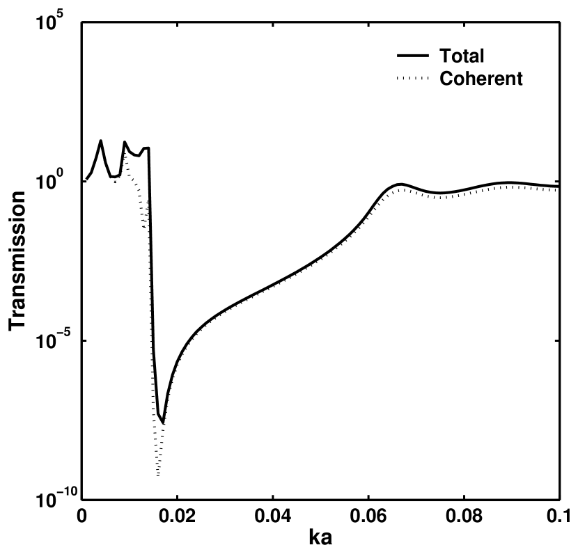
Figure 1: Transmissions as a function of $ka$.

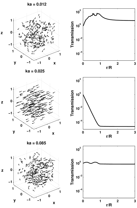
Figure 2: Left column: The phase diagram for the two dimensional phase vectors defined in the text for an arbitrary random distribution of bubbles. Right column: The acoustic energy distribution or transmission, averaged for all directions, as a function of distance away from the source; the distance is scaled by the sample size $R$. The three frequencies are selected from within and outside of the localization regime, referring to Fig. 1.

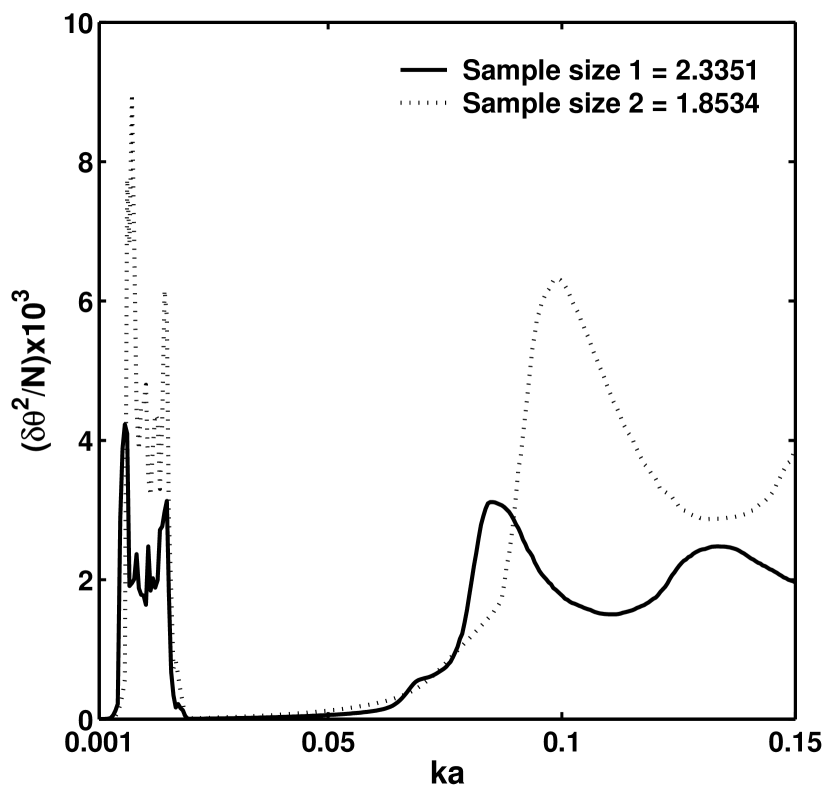
Figure 3: Fluctuation of the phase as a function of $ka$ for two sizes of bubble clouds. In both cases, the volume fraction is kept at 0.001.

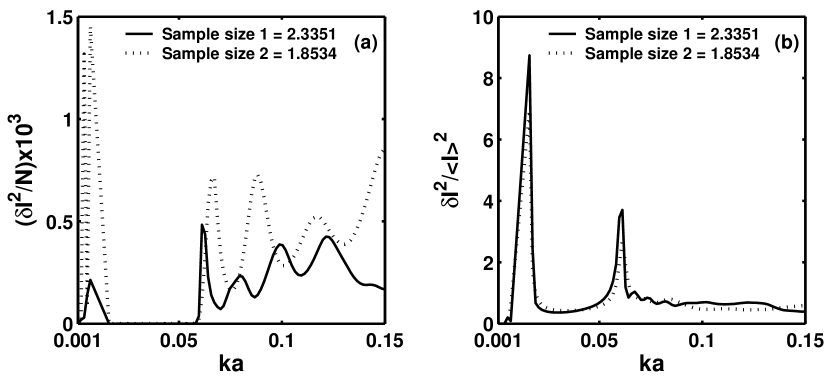
Figure 4: The fluctuation of transmission as a function of $ka$.

References

- (1) T. V. Ramakrishnan, Pramana - J. Phys. 56, No. 2, 149 (2002).
- (2) P. W. Anderson, Phys. Rev. 109, 1492 (1958).
- (3) P. A. Lee and Ramakrishnan, Rev. Mod. Phys. 57, 287 (1985).
- (4) D. J. Thouless, Phys. Rep. 13, 93 (1974).
- (5) M. Janssen, Fluctuations and localization (World Scientific, Singapore, 2001); and references therein.
- (6) S. John, Phys. Today, 44, 52 (1991).
- (7) P. Sheng, Introduction to Wave Scattering, Localization, and Mesoscopic Phenomena (Academic Press, New York, 1995).
- (8) A. Lagendijk and B. A. van Tiggelen, Phys. Rep. 270, 143 (1996).
- (9) R. Hennino, et. al., Phys. Rev. Lett. 86, 3447 (2001).
- (10) S. L. McCall, P. M. Platzman, R. Dalichaouch, D. Smith, and S. Schultz, Phys. Rev. Lett. 67, 2017 (1991).
- (11) R. D. Meade, A. M. Rapper, K. D. Brommer, J. D. Joannopoulos, and O. L. Alerhand, Phys. Rev. B 48, 8434 (1993).
- (12) D. S. Wiersma, P. Bartolini, A. Lagendijk, and R. Roghini, Nature 390, 671 (1997); F. Scheffold, R. Lenke, R. Tweer, and G. Maret, Nature 398, 206 (1999); D. S. Wiersma, J. Gomez Rivas, P. Bartolini, A. Lagendijk, and R. Roghini, Nature 398, 207 (1999).
- (13) Z. Ye and A. Alvarez, Phys. Rev. Lett. 80, 3503 (1998).
- (14) Z. Ye and H. Hsu, Appl. Phys. Lett. 79, 1724 (2001)
- (15) K. X. Wang and Z. Ye, Phys. Rev. E. 64, 056607 (2001).
- (16) E. Abraham and M. J. Stephen, J. Phys. C: Solid St. Phys. 13, L377 (1980).