Simulation and theory of vibrational phase relaxation in the critical and supercritical nitrogen: Origin of observed anomalies

Abstract

We present results of extensive computer simulations and theoretical analysis of vibrational phase relaxation of a nitrogen molecule along the critical isochore and also along the gas-liquid coexistence. The simulation includes all the different contributions [atom-atom (AA), vibration-rotation (VR) and resonant transfer] and their cross-correlations. Following Everitt and Skinner, we have included the vibrational coordinate ($q$) dependence of the interatomic potential. It is found that the latter makes an important contribution. The simulated results are in good agreement with the experiments. Dephasing time ($\tau_{\it v}$) and the root mean square frequency fluctuation ($\Delta$) in the supercritical region are calculated. The principal important results are: (a) a crossover from a Lorentzian-type to a Gaussian line shape is observed as the critical point is approached along the isochore (from above), (b) the root mean square frequency fluctuation shows nonmonotonic dependence on the temperature along critical isochore, (c) along the coexistence line and the critical isochore the temperature dependent linewidth shows a divergence-like $\lambda$-shape behavior, and (d) the value of the critical exponents along the coexistence and along the isochore are obtained by fitting. It is found that the linewidths (directly proportional to the rate of vibrational phase relaxation) calculated from the time integral of the normal coordinate time correlation function [$C_{Q}(t)$] are in good agreement with the known experimental results. The origin of the anomalous temperature dependence of linewidth can be traced to simultaneous occurrence of several factors, (i) the enhancement of negative cross-correlations between AA and VR contributions and (ii) the large density fluctuations as the critical point (CP) is approached. The former makes the decay faster so that local density fluctuations are probed on a femtosecond time scale. The reason for the negative cross-correlation between AA and VR is explored in detail. A mode coupling theory (MCT) analysis shows the slow decay of the enhanced density fluctuations near critical point. The MCT analysis demonstrates that the large enhancement of VR coupling near CP arises from the non-Gaussian behavior of density fluctuation and this enters through a nonzero value of the triplet direct correlation function.

I Introduction

The study of vibrational phase relaxation (VPR) has been an important endeavor of a physical chemist/chemical physicist in the attempt to understand and quantify the interaction of a chemical bond with the surrounding solvent molecules oxrev1 ; oxsim . As the phase relaxation of a bond is sensitive to the details of intermolecular interaction, it is a useful tool in understanding various aspects of solute-solvent interactions. The study of VPR has been driven by the sensitive experimental measurements of the vibrational linewidth. Thus the theoretical results can be verified with experiments directly. Simple models such as the isolated binary collisions model fish and hydrodynamic model oxrev1 were employed initially to explain the experimental results. These models led to simple expressions of temperature, density, and viscosity dependence of the rate. However, the agreement with experiments was at most tentative. It was soon realized that a major difficulty was that dephasing derives contributions from many sources and there may not be any unique mechanism of dephasing. Not only the estimation of these contributions are nontrivial, even the cross-correlations between different pure terms are non-negligible. Thus the Kubo theory of dephasing kubo was straightforward to apply in this case and the calculations of the frequency modulation time correlation function turned out to be extremely difficult, even for simple diatoms like nitrogen (N₂).

Uniqueness of vibrational dephasing near the critical point is that the value of mean square frequency fluctuation $\large<\Delta\omega^{2}(0)\large>$ becomes large, leading to rapid decay of $\large<Q(t)Q(0)\large>$. Many factors which are responsible for this behavior are very difficult to understand. Near high temperature vibration-rotational (VR) coupling shows large enhancement to $\large<\Delta\omega(t)\Delta\omega(0)\large>$ including negative cross-correlation between atom-atom and VR coupling terms.

Many experimental studies have been carried out on N₂ using vibrational Raman spectroscopy as a probe. Experimental studies of Clouter et al. clouter1 ; clouter2 showed that the isotropic Raman line shape of simple fluid like $N_{2}$ may exhibit a remarkable additional broadening near liquid-gas critical points ($\rho_{c},T_{c}$). They measured the Raman spectra along the triple point to the critical point and behavior of the line shape as the critical point is approached from above at a constant density. Recently Musso et al. musso calculated the important cross-correlations between resonant and nonresonant dephasing mechanisms in dense liquid. They observed an interesting temperature dependence $\lambda$ shaped linewidth ($\Gamma$) along the coexistence and along the critical isochore.

In their pioneering study, Oxtoby et al. oxrev1 ; oxsim ; oxrev2 showed that direct simulation of the vibrating molecules could be avoided for most cases of interest. A quantum mechanical perturbation theory for the vibrational motion can be used to express the dephasing rate in terms of auto- and cross-correlation functions of bond-force terms and its derivatives. The latter ones can then be calculated by molecular dynamics (MD) simulations. Oxtoby et al. calculated the linewidth and the motionally narrowed line shape of nitrogen near boiling point (77 K) fish ; oxrev2 . They considered several contributions from (i) solvent-solute interaction force in the liquid, (ii) their derivatives, and (iii) resonant molecular vibrational interactions to the frequency fluctuation of molecules.

Recently Gayathri et al. gay1 ; gay3 calculated the vibrational phase relaxation of the fundamental and the overtones tom1 ; tom2 of the N-N stretch of nitrogen in pure nitrogen by molecular dynamics (MD) simulations. They reproduced the experimental data semiquantitatively (within 40% in most cases). They have also applied the mode coupling theory (MCT) sarika1 ; swapan to compare with the simulation results. In their calculations they have not include the vibrational coordinate ($q$) dependence of the interatomic potential and also ignored the cross-terms among the vibration-rotation coupling term, the atom-atom term, and the resonance term. More recently Everitt and Skinner studied the Raman line shape of nitrogen in a systematic way by including the bond length dependence of the dispersion and repulsive force parameters eve . They have also included the cross-correlation terms which were neglected earlier and the results for the line shift and the linewidth along the liquid-gas coexistence of N₂ were observed to be in very good agreement with experiments. But calculations along the critical isochore have not been reported in their study. As mentioned earlier, there exists a profound experimental results in this region.

In this work, we report results of extensive MD simulations of vibrational dephasing along critical isochore. We have calculated the linewidth, the line shape, and the dephasing time of N₂ along the critical isochore and along the coexistence line. The normal coordinate time correlation function [$C_{Q}(t)$] is calculated from the frequency fluctuation time correlation function for different state points along the coexistence line as well as along the isochore of N₂.

We have incorporated the vibrational coordinate ($q$) dependency of the intermolecular potential and also the cross-terms. The linear expansion of the Lennard-Jones potential parameters on vibrational coordinate is very important to get the correct sign of line shift. The time integral of the diagonal and cross-terms of frequency fluctuation time correlation function [$C_{\omega}(t)$] gives the contribution to the linewidth. These cross-terms have a large effect on the linewidth to get a good agreement with experiment.

The line shape calculated from the normal coordinate time correlation function shows the Gaussian behavior close to the critical point. Experimentally musso , it has been proved that the line shape remains Lorentzian for the liquid near its normal boiling point (BP). The increase in density fluctuations near the critical point increases the mean square frequency fluctuation $\large<\Delta\omega^{2}_{i}\large>$, transferring the line shape from its fast modulation, i.e., Lorentzian shape limit outside the critical region to a slower modulated Gaussian shape. The root mean square (rms) frequency fluctuation of N₂ calculated along the isochore shows nonmonotonic behavior. However, the dephasing time ($\tau_{v}$) did not show any nonmonotonicity.

II Basic Expressions

The theories of the vibrational dephasing are all based on Kubo’s stochastic theory of the line shape. This gives a simple expression for the isotropic Raman line shape $[\it I(\omega)]$ in terms of Fourier transform of the normal coordinate time correlation function [$C_{Q}(t)$] through the polarizability time-correlation function as given by kubo ; kubo1 ,

$$I(\omega)=\int_{0}^{\infty}dt\exp(i\omega t)\left[\large<Q(t)Q(0)\large>\right].$$ (1)

A cumulant expansion of Eq. (1) followed by truncation after second order gives the following well known expression for $C_{Q}(t)$ (Ref kubo ):

$$C_{Q}(t) = \large<Q(t)Q(0)\large>$$ (2)

$$= Re\exp(i\omega_{0}t+i\large<\Delta\omega\large>t)$$

$$\times \exp\left[-\int_{0}^{t}dt^{\prime}(t-t^{\prime})\large<\Delta\omega(t^{\prime})\Delta\omega(0)\large>\right],$$

where $\Delta\omega_{i}(t)=\omega_{i}(t)-\large<\omega_{i}\large>$ is the fluctuation of the vibrational frequency from average vibrational frequency. $\large<\Delta\omega(t)\Delta\omega(0)\large>$ is the frequency fluctuation time correlation [$C_{\omega}(t)$] function and $\omega_{0}$ is the fundamental vibrational frequency of nitrogen.

The fluctuation in energy between the ground state and the $n$th quantum level of overtone transitions is given by

$$\hbar\Delta\omega_{n0}^{i}(t)=V_{nn}^{i}(t)-V_{00}^{i}(0)+\sum_{j}V_{ij}(t)~{}.$$ (3)

$V_{nn}^{i}$ is the Hamiltonian matrix element of the coupling of the vibrational mode to the solvent bath and $\sum_{j}V_{ij}(t)$ represents the contribution from resonant energy transfer between two molecules $i$ and $j$.

The Hamiltonian for the normal mode ($Q$) is assumed to be of the following anharmonic form:

$${\it H}_{vib}=\frac{1}{2}\mu\omega_{0}^{2}Q^{2}+\frac{1}{6}{\it f}Q^{3},$$ (4)

where $\mu$ is the reduced mass and $f$ is the anharmonic force constant. The value of $f$ is $17.8\times 10^{4}$ gm/cm s². Note that $Q$ in Eq. (4) is not in the mass-weighted form.

If $V$ is the oscillator-medium interaction potential, then one finds the following expression for the fluctuation in overtone frequency (by using perturbation theory) $\Delta\omega_{n0}(t)$ Ref (oxsim ):

$$\hbar\Delta\omega^{i}_{n0}(t) = (Q_{nn}-Q_{00})\left(\frac{\partial V}{\partial Q}\right)_{Q=0}(t)+\frac{1}{2}[(Q^{2})_{nn}-(Q^{2})_{00}]\left(\frac{\partial^{2}V}{\partial^{2}Q}\right)_{Q=0}(t)$$ (5)

$$+ Q^{2}_{n0}\sum_{j\neq i}\left(\frac{\partial^{2}V}{\partial Q_{i}Q_{j}}\right)_{Q=0}(t)+\ldots$$

$$= \left(\frac{{\it n}\hbar(-{\it f})}{2\mu^{2}\omega^{3}_{0}}\right){\it F}^{i}_{1Q}+\left(\frac{{\it n}\hbar}{2\mu\omega_{0}}\right){\it F}^{i}_{2Q}+\delta_{n1}\left(\frac{\hbar}{2\mu\omega_{0}}\right)^{\frac{1}{2}}\sum_{i\neq j}{\it F}^{\it i\it j}_{3Q}~{}.$$

The first two terms in the right-hand side of Eq. (5) are the atom-atom contributions and the third term is the resonance term.

The vibration-rotation (VR) contribution to the broadening of the line shape is given by $\Delta\omega_{n0,VR}=\Delta R_{n0}/\hbar{\it I}_{m}{\it r}_{e}.\Delta{\it J}^{2}$ schandler ; brueck ; where $\Delta{\it J}^{2}(t)={\it J}^{2}(t)-\large<{\it J}^{2}(0)\large>$. However, the time correlation function of VR coupling term is given by

$$C^{VR}_{\omega}(t) = \large<\Delta\omega(t)\Delta\omega(0)\large>_{n0,VR}$$ (6)

$$= \left(\frac{\Delta R_{n0}}{\hbar{\it I}_{m}{\it r}_{e}}\right)^{2}\times(\large<{\it J}^{2}(t){\it J}^{2}(0)\large>$$

$$-\large<{\it J}^{2}\large>^{2})~{}.$$

${\it J}$ is the angular momentum and ${\it I}_{m}$ is the moment of inertia value at the equilibrium bond length(${\it r}_{e}$).

Auto- and cross-correlations between atom-atom forces, VR coupling and resonance terms have been considered in our model. The final expression for $C^{total}_{\omega}(t)$ can thus be written as

$$C^{total}_{\omega}(t) = \large<\Delta\omega(t)\Delta\omega(0)\large>$$ (7)

$$= <\Delta\omega_{AA}(t)\Delta\omega_{AA}(0)\large>$$

$$+ \large<\Delta\omega_{VR}(t)\Delta\omega_{VR}(0)\large>$$

$$+ \large<\Delta\omega_{Rs}(t)\Delta\omega_{Rs}(0)\large>$$

$$+ \large<\Delta\omega_{AA}(t)\Delta\omega_{VR}(0)\large>$$

$$+ \large<\Delta\omega_{VR}(t)\Delta\omega_{Rs}(0)\large>$$

$$+ \large<\Delta\omega_{Rs}(t)\Delta\omega_{AA}(0)\large>~{}.$$

The line shape is obtained from the frequency fluctuation correlation function. ${\it F}^{i}_{1Q},{\it F}^{i}_{2Q}$ and ${\it F}^{i}_{3Q}$ in Eq. (5) and the VR coupling from Eq. (6) are calculated separately. The main difference from a previous calculation gay4 is that all the terms are vibrational coordinate dependent. This dependency comes through the bond length of the (r = r($q$)) molecule.

The Hamiltonian of homonuclear diatomic molecules can be expressed as the sum of three terms,

$${\rm H}={\rm H}_{\it v}+{\rm T}(\bf q)+{\rm U}(\bf q),$$ (8)

${\rm H}_{\it v}$ is the vibrational Hamiltonian. ${\rm T}(\bf q)$ is the total translational and rotational kinetic energy. ${\rm U}(\bf q)$ is the inter-molecular potential energy. ${\bf q}$ represents the collection of vibration coordinates $\{q_{\it i}\}$. The vibration Hamiltonian for the isolated (gas-phase) molecules is given by

$${\rm H}_{\it v}=\sum_{\it i}\left(\frac{{\it p}^{\rm 2}_{\it i}}{2\mu}+{\it u}(q_{\it i})\right).$$ (9)

Here $\sum$ represents the sum of all anharmonic oscillators for the vibrational modes of gas molecules. The conjugate momentum of $q_{\it i}$ is $p_{\it i}$ for the ${\it i}$th molecule of the oscillator. The translational and rotational kinetic energy term of the oscillator can be written as

$${\rm\vec{T}}(\bf q)=\sum_{\it i}\left(\frac{{\it\bf P}^{\rm 2}_{\it i}}{2M}+\frac{{\it\bf L}^{\rm 2}_{\it i}}{2{\rm I}(q_{\it i})}\right),$$ (10)

where ${\rm\bf P_{\it i}}$ and ${\rm\bf L_{\it i}}$ are the center of mass momentum and the angular momentum for molecule ${\it i}$, respectively and ${\rm I}(q)=\mu({\rm r}_{\it e}+q)^{2}$ is the moments of inertia. We can express ${\rm H}={\rm T}(0)+{\rm U}(0)$ as a bath Hamiltonian and the perturbation Hamiltonian V is given by, ${\rm V}={\rm T}(\bf q)+{\rm U}(\bf q)-{\rm T}(0)-{\rm U}(0)$. The total Hamiltonian

$${\rm H}={\rm H}_{\it v}+{\rm H}_{\it b}+{\rm V}.$$ (11)

The intermolecular potential energy can be written as

$${\rm U}(\bf{\rm q})=\frac{1}{2}\sum_{{\it i}\neq{\it j}}\sum_{\alpha\beta}{\it v}\\ (\epsilon_{\it ij},\sigma_{\it ij},{\bf{\rm r}}_{{\it i}\alpha{\it j}\beta}),$$ (12)

with

$${\bf r}_{i\alpha j\beta}={\bf{r^{\prime}}}_{j\beta}-{\bf r}_{i\alpha}\\ ={\bf r}_{j\beta}+\frac{q}{2}{\hat{\rm r}}_{j\beta}-{\bf r}_{i\alpha},$$ (13)

and

$${\vec{r^{\prime}}}_{j\beta}(\vec{q}_{\it j})={\vec{r}}_{j\beta}(0)+\frac{q}{2}{\hat{\rm r}}_{j\beta}.$$ (14)

Here ${\hat{\bf r}}_{j\beta}$ is the unit vector along $\beta$ atom of the vibrating molecule ($i$th molecule) from the center of mass (see Fig. 1).

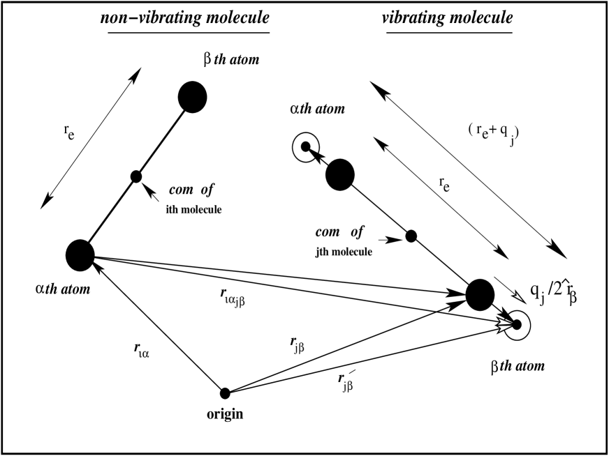
Figure 1: The schematic diagram illustrating molecular interactions between the nonvibrating ($i$th molecule) and vibrating ($j$th molecule) homonuclear diatomic (N₂).

III Simulation details

We have performed a microcanonical (NVE) ensemble molecular-dynamics (MD) simulation allen ; graphite at different state points of N₂ ranging from the melting point (also the triple point of N₂) through the boiling point and along the critical isochore (see Fig. 2) using the leap-frog algorithm fincham . The parameters used are given in  1 herz . A system of 256 $N_{2}$ diatomic molecules were enclosed in a cubic box and periodic boundary conditions were used.

Table 1: Parameters for $N_{2}$.

Potential parameters	$r_{o}/\AA$	1.094
	$\epsilon/kK$	37.3
	$\sigma/\AA$	3.31
Spectroscopic Constants	M/amu	28.0
	$\omega_{o}/cm^{-1}$	2358.57
Polarizability parameters	$\gamma/\AA^{-1}$	0.62
	$\delta/\AA^{-1}$	-0.063

Figure 2: Phase diagram of a typical substance, showing boundaries between solid (S), liquid (L) and vapor (G) or fluid (F) phases. This is only the projection of the $\rho^{*}-T^{*}$ plane. The parameters ($T^{*}_{c}$, $T^{*}_{t}$, $\rho^{*}_{c}$, and $\rho^{*}_{t}$) are given for nitrogen. We did the simulation along the critical isochore of nitrogen which is indicated by an arrow.

The thermodynamic state of the system is expressed in terms of the reduced number density of $\rho^{*}=\rho\sigma^{3}$ (Ref. allen ) and a reduced temperature of $T^{*}=k_{B}T/\epsilon$. $\sigma$ is the diameter of the molecule and $\epsilon$ is the interaction parameter (see 1). The unit of temperature is $\epsilon/k_{B}$ (K), where $k_{B}$ is the Boltzmann constant. Cheung and Powels cheung had earlier studied liquid N₂ at different state points using MD simulations. Most of the thermodynamic state points chosen for the work presented here have been taken from their study. We have done few simulations with a system of 512 nitrogen molecules to check the system size dependency.

Fig. 2 gives a schematic view of the phase diagram balzop . The arrowed line points out that along the critical isochore, $T_{c}$ is approached from above. For nitrogen the triple point corresponds to that given by ($T^{*}_{t},\rho^{*}_{t})=(1.7212,0.6964$) and the critical point, $(T^{*}_{c},\rho^{*}_{c})=(3.3592,0.35)$.

For intermolecular potential-energy (${\it V}_{\it ij}$) between two molecules i and j, the following site-site Lennard-Jones type is employed as given below,

$${\rm V}_{\it ij}=\sum_{\alpha,\beta}^{\it 1,2}{\rm V}({\rm r}_{i\alpha j\beta}).$$ (15)

Here ${\rm V}({\rm r}_{i\alpha j\beta})$ is the Lennard-Jones atom-atom potential defined as

$${\rm V}({\rm r}_{i\alpha j\beta})=4{\epsilon}_{i\alpha j\beta}[(\frac{{\it\sigma}_{i\alpha j\beta}}{{\rm r}_{i\alpha j\beta}})^{12}-(\frac{{\sigma}_{i\alpha j\beta}}{{\rm r}_{i\alpha j\beta}})^{6}].$$ (16)

Vibrational coordinate dependence of $\epsilon$ and $\sigma$ has been incorporated following Everitt and Skinner eve ,

$$\epsilon(q) = \epsilon[1+2\gamma q];$$

$$\sigma(q) = \sigma[1+2\delta q].$$ (17)

For homonuclear diatomic-like nitrogen,

$$\epsilon_{i\alpha j\beta} = \sqrt{\epsilon_{i\alpha}\epsilon_{j\beta}}$$ (18)

$$= \epsilon_{ij},$$

$$\sigma_{i\alpha j\beta} = \frac{\sigma_{\alpha\alpha}+\sigma_{\beta\beta}}{2}$$ (19)

$$= \sigma_{ij},$$

and

$$\epsilon_{ij}\simeq\epsilon(1+\gamma q_{i}+\gamma q_{j}+2\gamma^{2}q_{i}q_{j}),$$ (20)

$$\sigma_{ij}=\sigma(1+\delta q_{i}+\delta q_{j}).$$ (21)

Now the LJ potential takes the form as below,

$${\rm V}_{ij} = \sum_{\alpha,\beta=1}^{2}\large[4\epsilon\{1+\gamma(q_{i}+q_{j})+2\gamma^{2}q_{i}q_{j}\}$$ (22)

$$\times\large\{\large(\frac{\sigma}{\rm r_{i\alpha j\beta}}\large)^{12}(1+\delta q_{i}+\delta q_{j})^{12}$$

$$-\large(\frac{\sigma}{\rm r_{i\alpha j\beta}}\large)^{6}(1+\delta q_{i}+\delta q_{j})^{6}\large\}\large].$$

IV Simulation Results, Comparison with Experiment and Discussion

IV.1 Along the coexistence line

The frequency-modulation time correlation function [$C_{\omega}(t)$], the dephasing linewidth, and the line shift amot are all obtained for several thermodynamic state points ranging from triple point to critical point.

We have calculated the line shift $\Delta\nu^{~{}}=(\left<\omega_{i}\right>-\omega_{0})/2\pi c$ as a function of density for nitrogen. The magnitude of the line shift increases with density as clearly seen in Fig. 3(a) and the results are in good agreement with the experiment. The vibrational coordinate dependence is important to get the correct sign of the line shift.

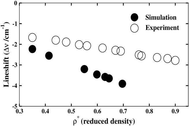
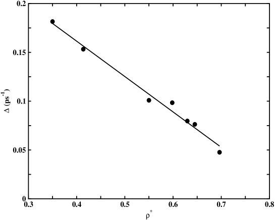
Figure 3: The Raman line shift ($\Delta\nu$) is plotted against density ($\rho^{*}$) ($a$) along the coexistence line for N₂. The critical density is indicated by the arrow. The rms frequency fluctuation $\Delta$ is plotted against reduced density ($b$) along the coexistence line for N₂. Simulation results have been fitted with the formula $y=ax+b$ with $a=-0.3624$ and $b=0.3064$.

Along the coexistence line the root mean square frequency fluctuation ($\Delta$) increases as the critical point is approached. Fig. 3(b) shows that $\Delta$ decreases linearly with density with a slope of -0.3624.

IV.2 Along the critical isochore

We have plotted $C_{\omega}(t)$ against time for three different temperatures along the critical isochore in Fig. 4. The lines with open circles show $C_{\omega}(t)$ which decays faster than $C_{\omega}(t)$ represented by the simple line.

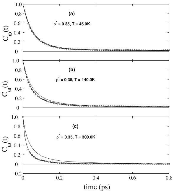
Figure 4: The frequency fluctuation time correlation functions [$C_{\omega}(t)$] are plotted against time (t) at different temperatures (a) T = 45.0 K, (b) T = 140.0 K, and (c) T = 300.0 K along the critical isochore. In all the figures above, circles with a simple line show $C_{\omega}(t)$ for $q$ dependent interaction potential, whereas the simple solid line shows the $q$ independent interaction potential.

The temperature dependence of the dephasing time ($\tau_{v}$) calculated by integration of $C_{\omega}(t)$ [Eq. 7] is comparable with experimental results (see 2).

Table 2: Simulated values of Dephasing time at different temperatures.

	$\tau_{v}$(ps)
Temperature(K)	Simulation	Expt
125.3	12.40	14.5
140.0	19.06	23.3
149.3	25.13	27.8
170.0	26.62	28.6
186.5	26.75	26.7

In Fig. 5, a simple line represents the normal coordinate time correlation function without including $q$ dependency of LJ parameters whereas the dashed line represents the same results with $q$ dependent LJ parameters. The former one has a larger correlation time than the latter one. The $C_{Q}(t)$ clearly shows the importance of $q$ dependence.

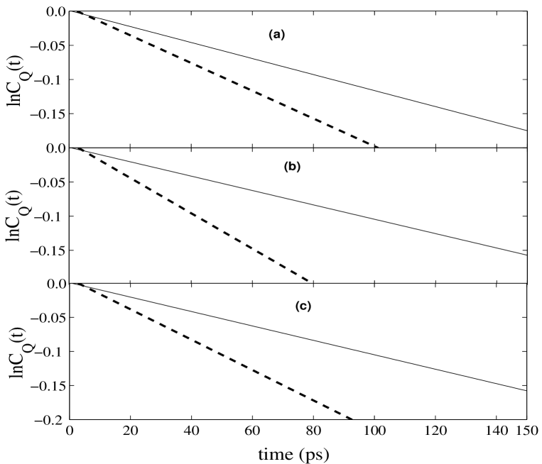
Figure 5: The normal coordinate time correlation functions [$C_{Q}(t)$] are plotted against time ($t$) at three temperatures along the critical isochore (a) T = 110.8 K, (b) T = 125.3 K, and (c) T = 140.0 K.

Fig. 6 displays the root mean square frequency fluctuation $\Delta$ [$=\sqrt{\Delta\omega^{2}(0)}$] calculated from unnormalized $C_{\omega}(0)$ at different temperatures along the isochore. The calculated $\Delta$ shows a nonmonotonic behavior with temperature. $\Delta$ initially increases with temperature and shows a maximum near critical temperature indicated by an arrow. A sharp decrease is observed for the temperature greater than $T_{c}$. The increase in density fluctuation near the critical point is responsible for this nonmonotonic behavior of rms frequency fluctuations.

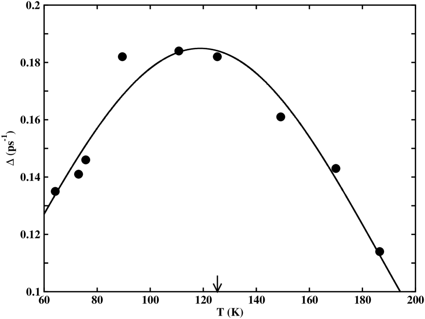
Figure 6: The rms frequency fluctuation $\Delta$ vs temperature (T) along the critical isochore for N₂. We fitted all simulation points with Gaussian. The fitting formula is $y=a[e^{-b(x-c)^{2}}]$, where $a=0.184904,b=0.00010813,andc=118.874.$

Table 3: Temperature dependence $\lambda$ shaped linewidth along the coexistence and critical isochore.

Temperature(K)	Linewidth(Ghz)
64.2	2.764
71.6	2.802
75.7	2.809
89.5	2.812
110.8	2.812
120.0	6.965
125.3	16.12
135.0	12.38
140.0	10.49
149.2	7.96
170.0	7.51
186.5	7.47

Linewidth shows an interesting $\lambda$-shaped feature when it is plotted against temperature (see 3) for the two different branches of calculation for N₂ as shown in Fig. 7. This figure is very similar to the one observed in experiment (see Fig. 4 of Ref musso ). It is interesting to note the sharp rise in the dephasing rate as the critical point is approached. There are six main contributions, (a) density [$C^{\rho}_{\omega}(t)$], (b) VR coupling [$C^{VR}_{\omega}(t)$ ], (c) resonance [$C^{Rs}_{\omega}(t)$], (d) density-VR coupling [$C^{\rho-VR}_{\omega}(t)$], (e) density-resonance [$C^{VR-Rs}_{\omega}(t)$], and (f) VR-resonance [$C^{\rho-Rs}_{\omega}(t)$] which are responsible for the sharp rise in total linewidth near the critical point. These are the time integrals of diagonal and cross-terms in the frequency fluctuation time correlation function. We shall come back to this point a bit later.

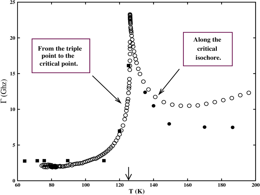
Figure 7: The lambda ($\lambda$) shaped linewidth ($\Gamma$) of nitrogen along the coexistence line (closed square) and the critical isochore (closed circle). The experimental results for linewidth along the coexistence line and the critical isochore (open circle) reported by Musso et al. in Ref. musso are also shown. The critical point is indicated by an arrow on the abscissa.

A crossover from Lorentzian-type line shape to Gaussian line shape is found to take place when there is a large separation in the time scales of decay of $C_{\omega}(t)$ and $C_{Q}(t)$ musso ; oxrev2 cease to exist and the two time correlation functions begin to overlap. We have calculated $C_{\omega}(t)$ and $C_{Q}(t)$ at three temperatures near the critical point (see Fig. 8). The decay of $C_{\omega}(t)$ becomes significantly faster, reducing the gap of decay between the two correlation functions. Indeed, the computed line shape becomes Gaussian near the critical point but otherwise remains Lorentzian-type both above and below the critical temperature. Note that the frequency modulation time correlation function decays fully in about 200 fs.

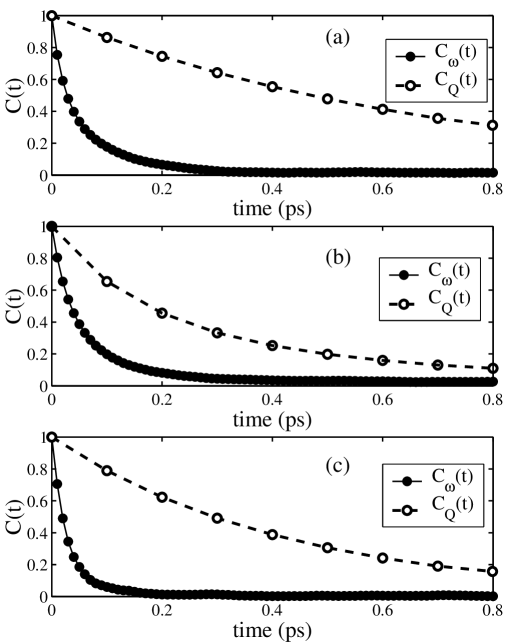
Figure 8: The frequency fluctuation time correlation function, $C_{\omega}(t)$, and the normal coordinate time correlation function, $C_{Q}(t)$, are plotted at (a) 186.5 K, and (b) 140.0 K (along critical isochore), and (c) the $C_{\omega}(t)$ and $C_{Q}(t)$ are plotted along the coexistence line at temperature 75.7 K.

To understand the origin of this critical behavior, we have carefully analyzed each one of the six terms which consist of three autocorrelations and three cross-terms between density, vibration-rotation coupling, and resonance terms which have been mentioned earlier.

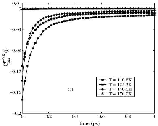
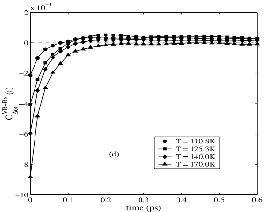
Figure 9: The decopositions of unnormalized frequency fluctuation time correlation functions for N₂ into (a) density-density, (b) VR-VR coupling, (c) density-VR and (d) VR-resonance at four temperatures along the critical isochore. The density-resonance and resonance-resonance terms are relatively small and are not shown here.

Fig. 9 shows the time dependence of the four dominating terms , the two autocorrelations [Fig. 9(a) and Fig. 9(b)] and two cross-correlations (Fig. 9(c) and Fig. 9(d)). The decompositions of line shift, linewidth, and the temperature dependent quantities are fully dependent on the contributions which come from all six terms. As we approach the critical point along the critical isochore, the magnitude of contributions from different terms are increased. Results for only four different temperatures including the critical point are shown in Fig. 9. All the remaining terms, resonance-resonance and density-resonance, are found to be unimportant in comparison with these four terms.

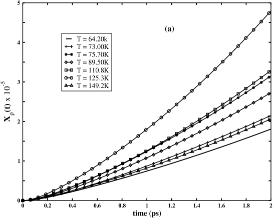
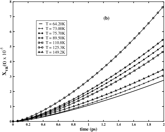
Figure 10: The time dependence of the relative contributions of the (a) density-density, $X_{den}(t)$, and (b) VR coupling, $X_{VR}(t)$, terms at different temperatures along the critical isochore.

The time dependence relative contribution $X_{ij}(t)=\int_{0}^{t}dt^{\prime}(t-t^{\prime})C_{\omega}^{ij}(t^{\prime})$ of the density [Fig. 10a] and vibration-rotation coupling term (Fig. 10b) are plotted for seven state points along the critical isochore, which are found to be dominant near the critical point. The sharp rise in the value of the integrand as the critical temperature is approached and the fall when it is crossed. We have found that both these contributions at the critical point are distinct compared to the other state points. Thus the rise and fall of the dephasing rate arise partly from the rise and fall in the density and the vibration-rotation terms. We have calculated the slopes of the relative contributions by the linear fitting in the long time at a particular temperature $T$ = 125.3 K. The values of the slope are $5.4\times 10^{-5}$, $9.5\times 10^{-5}$ and $-6.8\times 10^{-5}$ for density-density, VR-VR coupling, and density-VR terms, respectively. The major contribution comes from the VR coupling term among the four dominating terms.

V Dynamical heterogeneities near the critical point.

We have investigated the presence of dynamical heterogeneities in the fluid to further explore the origin of these anomalous critical temperature effects stanley ; ma . This can be quantified by the well-known non-Gaussian parameter $\alpha(t)$. It is defined as ara

$$\alpha(t)=\left(\frac{3}{5}\right)\frac{<r^{4}(t)>}{<r^{2}(t)>^{2}}-1,$$ (23)

where $\large<\Delta r(t)^{2}\large>$ is the mean squared displacement and $\large<\Delta r(t)^{4}\large>$ the mean quartic displacement of the center of mass of the nitrogen molecule. It can only approach zero (and hence Gaussian behavior) at a time scale larger than the time scale required for individual particles to sample their complete kinetic environments. The function $\alpha$(t) is large near the critical point at times 0.5-5 ps as observed in Fig. 11 which indicates the presence of long lived heterogeneities near $T_{c}$.

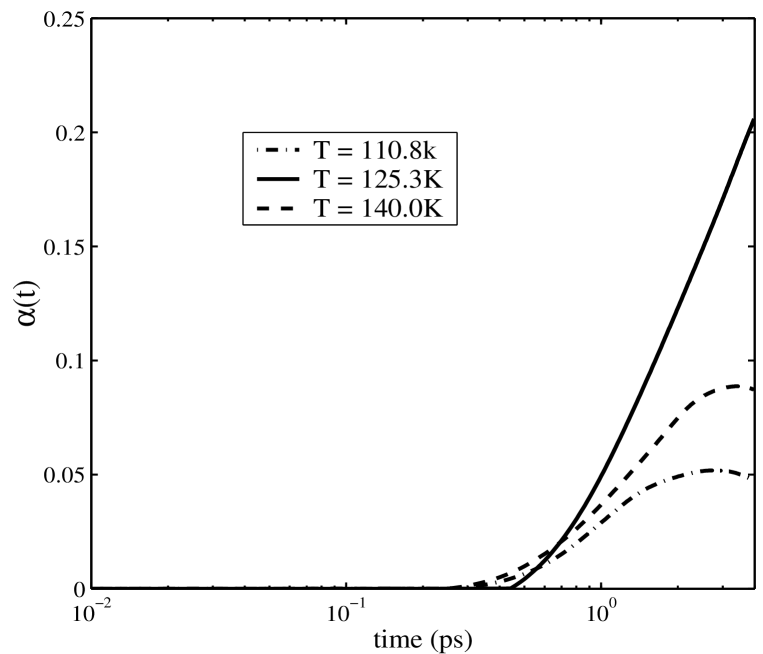
Figure 11: The non Gaussian parmeter $\alpha(t)$ is plotted against time ($t$) at three different temperatures along the critical isochore.

VI Negative cross-correlation between the density and VR coupling term

The role of cross-terms (which can be negative) are extremely important for the decay of $C_{\omega}(t)$ which occurs in the femtosecond time scale along the critical isochore. We have calculated the cross-terms among density, VR coupling, and resonance term. The cross-terms of VR coupling with density and resonance are found to be negative [see Figs. 9(c) and 9(d)]. As mentioned earlier the major contributions to the frequency fluctuation come from the density as well as from the VR coupling term. One of the main reasons for ultrafast decay of $C_{\omega}$ is the cancellations of negative cross-terms from the total contribution.

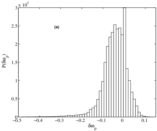
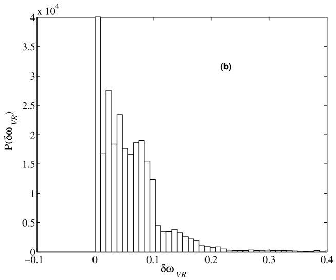
Figure 12: The distribution of fluctuation in (a) the density term, and (b) the VR coupling contribution to total fluctuation in the frequency at the temperature 110.8 K.

Now the question is why are these cross-terms are negative? The distribution of density dependent and the VR coupling dependent part of the total frequency fluctuation along the isochore are shown in Figs. 12(a) and 12(b), respectively. The peak of those distributions is near zero $\delta\omega_{VR}$ which proves that the homogeneity condition is satisfied along the isochore. It is evident that the distribution of $\delta\omega_{VR}$ is always positive while the distribution of $\delta\omega_{\rho}$ showed the long negative tail. The distribution of the product of density and VR coupling terms are plotted for different temperatures in Fig. 13. It is clearly seen that this distribution is negative. A detailed analysis of the origin of the negative sign of the cross-correlation between AA and VR coupling terms is given in Appendix B. On the other hand $\Delta\omega_{\rho}$ is directly proportional to the force acting on the bond of the diatoms. If force $F$ is large, the velocity will be large and it reflects that the $J^{2}$ will be decreased when $F$ is increased and vice versa. This is the origin of anticorrelation between the density and VR coupling terms in $C_{\omega}(t)$.

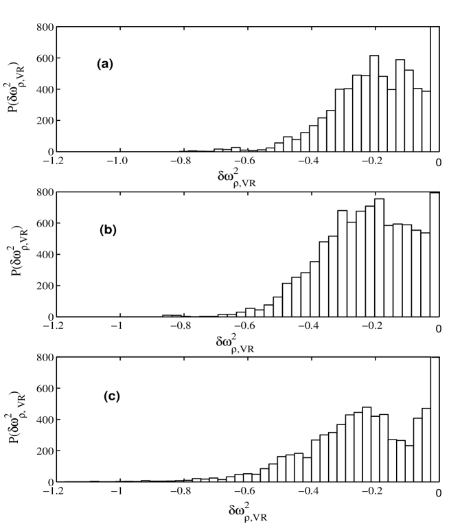
Figure 13: The distribution of correlation between density-VR coupling at three temperatures, (a) 110.8 K, (b) 125.3 K and (c) 140.0 K, respectively. Note that this figure is entirely different from Fig. 14.

The distribution of correlation between the density-density term and the VR-VR coupling term in the frequency fluctuation time correlation function are shown in Figs. 14(a) and 14(b), respectively. Both distributions are positive and the homogeneity condition of frequency fluctuations is satisfied in both cases.

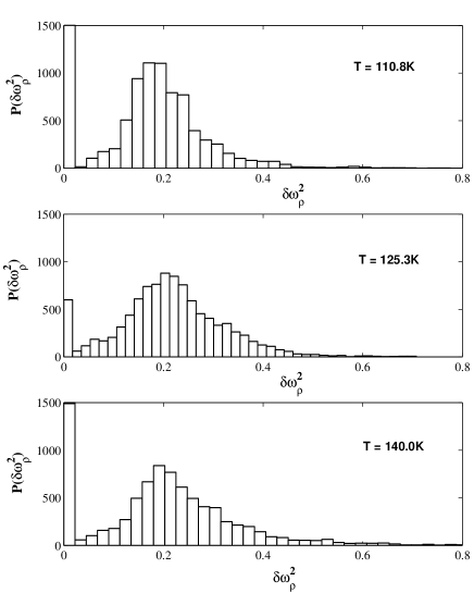
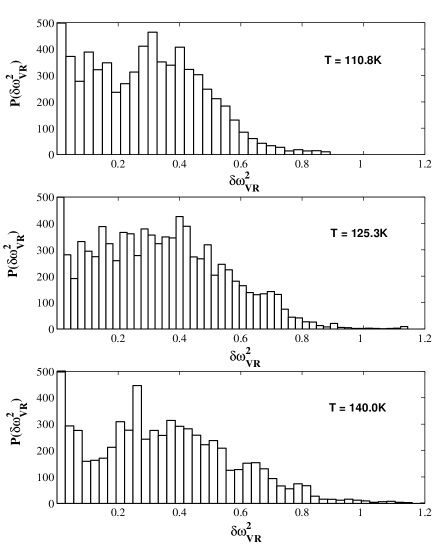
Figure 14: The distribution of (a) the density-density term and (b) the VR-VR coupling at term three temperatures 110.8 K, 125.3 K and 140.0 K respectively.

VII Mode Coupling Theory Analysis.

We can use mode coupling theory to obtain an expression for the atom-atom contribution to the frequency modulation time correlation function. The main steps have already been discussed by Gayathri et al. gay3 and need not be repeated here. In brief, MCT gives the following expression for the density dependent frequency modulation time correlation function sarika considering that the number density is the only relevant slow variable in dephasing,

$$\left<\Delta\omega_{\rho}(0)\Delta\omega_{\rho}(t)\right>=\frac{(k_{B}T)^{2}}{6\pi^{2}\hbar^{2}\rho}\int_{0}^{\infty}k^{2}dkF_{s}(k,t)c^{2}(k)F(k,t).$$ (24)

Where $c(k)$ is the Fourier transform of the two particle direct correlation function. The main contribution is derived from the long wavelength (that is small $k$) region near the critical point (CP). In the small $k$ limit the hydrodynamic expressions for two-point correlation functions are given by

$$F_{s}(k,t)=e^{-D_{s}k^{2}t},$$ (25a)

$$F(k,t)=S(k)e^{-D_{T}k^{2}t},$$ (25b)

where $F_{s}(k,t)$ is the self-intermediate scattering function and $F(k,t)$ is the intermediate scattering function. Here $D_{s}$ is the self-diffusion coefficient, $S(k)$ is the static structure factor, and $D_{T}$ is the thermal diffusivity. Thus $\left<\Delta\omega_{\rho}(0)\Delta\omega_{\rho}(t)\right>\simeq S(k\rightarrow 0)e^{-(D_{s}+D_{T})k^{2}t}$. Near the CP, $S(k\rightarrow 0)$ becomes very large ( as compressibility diverges at $T=T_{c}$ ), leading towards a Gaussian behavior for line shape. $D_{T}$ also undergoes a slowdown near $T_{c}$. However, a limitation of the above analysis is the absence of the VR term which contributes significantly and may mask some of the critical effects.

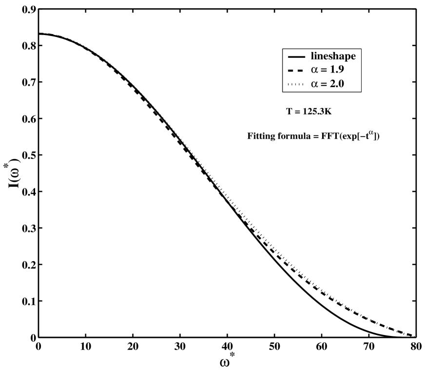
Figure 15: The behavior of line shape at the temperature 123.5 K.

All these lead to a large value of $\large<\Delta\omega^{2}(0)\large>$, which may lead to a Levy distribution from time dependence of $\left<Q(0)Q(t)\right>$ as discussed earlier by Mukamel et al. muk . At high temperature, the latter dominates over the density term. We have calculated the line shape and fitted with the Fourier transform of Levy distribution ( see Fig. 15). Clearly as $T_{c}$ is approached, the low $k$ fluctuations become more important and, if the high $k$ contributions are sufficiently small, they will dominate the line shape. We would like to mention that the line shape becomes Gaussian (see the Fig. 15) instead of the Fourier transform of Levy distribution near the critical point. The small $k$ picture described here is quite from the usual collisional broadening picture of dephasing. A complete Lorentzian behavior is predicted only in the low temperature liquid phase. Interestingly, the predicted divergence of $\large<\Delta\omega^{2}(0)\large>$ very close to $T_{c}$ enhances the rate of dephasing and this shifts the decay of $\large<Q(t)Q(0)\large>$ to short times, which gives rise to the Gaussian behavior.

We next use MCT to analyze the cross-correlation between VR coupling and the atom-atom ($\Delta\omega_{\rho}$) term. According to density functional theory (DFT) the effective potential energy ($V_{eff}$) of the mean field force $\left[{\bf F}=-{\bf\nabla}V_{eff}({\bf r},t)\right]$ can be written in terms of the two-particle correlation function $c({\bf r})$ without including orientation(${\bf\Omega}$) as

$$\beta V_{eff}({\bf r},t)=-\int d{\bf r^{\prime}}c({\bf r}-{\bf r^{\prime}})\delta\rho({\bf r^{\prime}},t).$$ (26)

Assuming that the density term is approximated by the isotropic limit, we can therefore write the atom-atom terms as

$$\Delta\omega_{\rho}({\bf r},t)=-k_{B}T/\hbar\int d{\bf r^{\prime}}c({\bf r}-{\bf r^{\prime}},t)\delta\rho({\bf r^{\prime}},t).$$ (27)

The calculation of the VR term is a bit more complicated. The angular momentum ${\bf J}(t)$ at time $t$ can be expressed in terms of torque ${\bf N}(t^{\prime})$ at earlier times ($t^{\prime}>t$),

$${\bf J}(t)={\bf J}(0)+\int dt^{\prime}{\bf N}(t^{\prime}).$$ (28a)

From Eq. 38 of the Appendix B, the VR coupling can be written as

$$\Delta\omega_{VR}({\bf r},{\bf\Omega},t)=A{\bf J}({\bf r},{\bf\Omega},t)\cdot{\bf J}({\bf r},{\bf\Omega},t)=A\large[J^{2}({\bf r},{\bf\Omega},0)+2\int dt^{\prime}{\bf J}({\bf r},{\bf\Omega},0)\cdot{\bf N}({\bf r},{\bf\Omega},t^{\prime})$$

$$+\int dt^{\prime}\int dt^{\prime\prime}{\bf N}({\bf r},{\bf\Omega},t^{\prime})\cdot{\bf N}({\bf r},{\bf\Omega},t^{\prime\prime})\large].$$ (28b)

Here $A$ is a constant (see Appendix B) and $\delta\rho({\bf r^{\prime}},{\bf\Omega^{\prime}},t^{\prime})$ is the fluctuation in the number density.

The expression for the cross-correlation can be expressed as

$$\left<\Delta\omega_{VR}({\bf r},{\bf\Omega},t)\Delta\omega_{\rho}({\bf r},0)\right>=-A(k_{B}T/\hbar)\large[\int d{\bf r^{\prime}}c({\bf r}-{\bf r^{\prime}})\left<J^{2}({\bf r},{\bf\Omega},0)\delta\rho({\bf r^{\prime}},0)\right>$$

$$+2\int dt^{\prime}\int d{\bf r^{\prime}}c({\bf r}-{\bf r^{\prime}})\left<{\bf J}({\bf r},{\bf\Omega},0)\cdot{\bf N}({\bf\Omega},t^{\prime})\delta\rho({\bf r^{\prime}},0)\right>$$

$$+\int dt^{\prime}\int dt^{\prime\prime}\int d{\bf r^{\prime}}c({\bf r}-{\bf r^{\prime}})\left<{\bf N}({\bf\Omega},t^{\prime})\cdot{\bf N}({\bf\Omega},t^{\prime\prime})\delta\rho({\bf r^{\prime}},0)\right>\large].$$ (29)

By using DFT again, the torque (${\bf N}$) can expressed in terms of density functions as

$${\bf N}({\bf r},{\bf\Omega},t)={\bf\nabla}_{\bf\Omega}\int d{\bf r^{\prime}}d{\bf\Omega^{\prime}}c({\bf r}-{\bf r^{\prime}},{\bf\Omega},{\bf\Omega^{\prime}})\delta\rho({\bf r^{\prime}},{\bf\Omega^{\prime}},t).$$ (30)

Combining the above equations, the final expression cross-correlation can be written as,

$$<\Delta\omega_{VR}({\bf r},{\bf\Omega},t)\Delta\omega_{\rho}({\bf r},0)>=-A(k_{B}T/\hbar)\Large[\int d{\bf r^{\prime}}c({\bf r}-{\bf r^{\prime}})\left<J^{2}({\bf r},{\bf\Omega},0)\delta\rho({\bf r^{\prime}},0)\right>$$

$$+2\int dt^{\prime}\int d{\bf r^{\prime}}\int d{\bf r^{\prime\prime}}d{\bf\Omega^{\prime}}c({\bf r}-{\bf r^{\prime}}){\bf\nabla_{\Omega^{\prime}}}\cdot c({\bf r}-{\bf r^{\prime\prime}},{\bf\Omega},{\bf\Omega^{\prime}})\left<{\bf J}({\bf r},{\bf\Omega},0)\delta\rho({\bf r^{\prime\prime}},{\bf\Omega^{\prime}},t^{\prime})\delta\rho({\bf r^{\prime}},0)\right>$$

$$+\int dt^{\prime}\int dt^{\prime\prime}\int d{\bf r^{\prime\prime}}d{\bf\Omega^{\prime}}\int d{\bf r^{\prime\prime\prime}}d{\bf\Omega^{\prime\prime}}\int d{\bf r^{\prime}}c({\bf r}-{\bf r^{\prime}}){\bf\nabla_{\Omega^{\prime}}}\cdot{\bf\nabla_{\Omega^{\prime\prime}}}c({\bf r}-{\bf r^{\prime\prime}},{\bf\Omega},{\bf\Omega^{\prime}})c({\bf r}-{\bf r^{\prime\prime\prime}},{\bf\Omega},{\bf\Omega^{\prime\prime}})$$

$$\times\left<\delta\rho({\bf r^{\prime\prime}},{\bf\Omega^{\prime}},t^{\prime})\delta\rho({\bf r^{\prime\prime\prime}},{\bf\Omega^{\prime\prime}},t^{\prime\prime})\delta\rho({\bf r^{\prime}},0)\right>\Large]$$

$$\equiv{\bf I+II+III}.$$ (31)

We now analyze Eq. (31) term by term. Since both $J$ and $\delta\rho$ are uncoupled at the same time, the contribution of I is zero. The second term II in Eq. (31) consists of two density terms with an angular momentum term. Using cumulant expansion we can show that the contribution of II is also equal to zero.

To evaluate the third term (III), we factorize the translational and angular variables in the two-particle direct correlation function (DCF) and we can write

$$c({\bf r}-{\bf r^{\prime}},{\bf\Omega},{\bf\Omega^{\prime}})=c_{\theta}({\bf\Omega},{\bf\Omega^{\prime}})c_{0}(|{\bf r}-{\bf r^{\prime}}|).$$ (32)

Where $c_{0}(|{\bf r}-{\bf r^{\prime}}|)$ is the isotropic part of the direct correlation function. When the temperature $T\rightarrow T_{c}$, $c_{0}\rightarrow\rho_{0}^{-1}$, which is finite. The angular part of the direct correlation function $c_{\theta}({\bf\Omega},{\bf\Omega^{\prime}})$ can be expanded in terms of the spherical harmonics.

$$c_{\theta}({\bf\Omega},{\bf\Omega^{\prime}})=\sum_{l_{1},l_{2},m}a_{l_{1}l_{2}m}{\bf Y}_{l_{1},m}({\bf\Omega}){\bf Y}_{l_{2},m}({\bf\Omega^{\prime}}).$$ (33)

If we assume that the density effects are included in the spatial part $c_{0}(|{\bf r}-{\bf r^{\prime}}|)$ then the final expression of the angular part of the direct correlation function will be finite and nonzero. If one assumes that the $\delta\rho$ are Gaussian random variables, then the value of the triplet correlation function in III is zero, by cumulant expansion. However, the distribution of the fluctuation in number density clearly shows a non-Gaussian behavior, arising from the long lived heterogeneity near critical point (see Fig. $11$). We, therefore, expect a nonzero value of the cross-correlation between VR coupling and atom-atom terms from the triplet correlation function in Eq. (31). Moreover, the amplitude of the cross-correlation is predicted to be small at all temperatures away from $T_{c}$ but it is predicted to become significant as $T_{c}$ is approached, where the density fluctuation becomes non-Gaussian.

We have calculated the term $\Delta R$ in Eq. 38 (see Appendix B) and found it to be always positive. It is obvious that $J^{2}>0$. So we can conclude that $\delta\omega_{VR}>0$ [see Fig. $12b$]. Figure $12(a)$ shows that most of the distribution of fluctuation in $\delta\omega_{\rho}$ are in the negative direction. On the other hand the distribution of fluctuation in $\delta\omega_{VR}$ is in the positive direction [see Fig. $12b$]. Here, $\Delta\omega_{\rho}=\left({\it n}\hbar(-{\it f})/2\mu^{2}\omega^{3}_{0}\right){\it F}^{i}_{1Q}+\left({\it n}\hbar/{2\mu\omega_{0}}\right){\it F}^{i}_{2Q}.$ So the distribution of cross-correlation between density and VR coupling terms must be negative (see Fig. $13$).

The above analysis MCT demonstrates that the large enhancement of vibration-rotation coupling near the gas-liquid critical point arises from the non-Gaussian behavior of density fluctuation and this enters through a nonzero value of the triplet direct correlation function [Eq. (31)].

VIII Divergence of Raman linewidth near the CP

Along the coexistence line and the critical isochore, we have found that the temperature dependence of the linewidth ($\Gamma$) is singular near the critical point. The divergence-like rise near $T_{c}$ is fitted to a form $(T-T_{c})^{-\beta^{\prime}}$. From the fitting with both experimental and theoretical data we have found $\beta^{\prime}=0.386$ along the coexistence line and $\beta^{\prime}=0.207$ along the critical isochore.

Above $T_{c}$, the fluctuations swapan are small which cause the resonance lines to be homogeneously broadened and the line shape is Lorentzian. On approaching $T_{c}$, the fluctuations md1 ; md2 become large and their correlation time also increases, as a consequence the line shape becomes Gaussian.

The order parameter for the liquid-gas critical point is $(\rho_{L}-\rho_{G})$. This goes to zero as $(T_{c}-T)^{-\beta}$ where $\beta\simeq\frac{1}{3}$. Mukamel et al. muk have studied the broadening of spectral lines by using mode-coupling theory ks ; fixman near a liquid-gas critical point. They assumed Lorentzian form of the line and found that the linewidth increases with $\epsilon^{-s}$, where $\epsilon=|(T-T_{c})/T_{c}|$. They have also found that the value of critical exponent (s) changes from 0.607 for large $\epsilon$ to $0$ for small $\epsilon$. That is, the singularity becomes weaker as $T_{c}$ is approached. It is likely that simulations are not sufficiently close to $T_{c}$ because simulations are finite sized.

The reason for the relative success of a small system in reproducing experimental behavior is that dephasing probes only local static fluctuations. Thus long range static and dynamic correlations important in specific heat, compressibility, or light scattering are not relevant in vibrational dephasing. Second, while our simulated system can certainly capture the increase in fluctuation, it can never capture the long range fluctuations. But it captures enough to reproduce many of the features. Note that even a small system is capable of exhibiting large fluctuations near the gas-liquid coexistence/critical point. Put bluntly, truly large scale critical fluctuations are neither required nor reflected for dephasing simply because dephasing is a local process.

IX Conclusion

In this article extensive MD simulations of vibrational phase relaxation of nitrogen have been presented. The simulations reported here seem to reproduce many of the anomalies observed in experiments. It shows (a) the origin of enhanced negative cross-correlations, (b) a crossover from a Lorentzian-type to a Gaussian line shape as the critical point is approached, (c) the non-monotonic dependence of rms frequency fluctuation on temperature along the critical isochore, (d) a lambda shaped dependence of linewidth on temperature, and (e) a near divergence of linewidth near the critical point.

X Acknowledgment

One of us (S.R.) would like to thank A. Mukherjee, Prasanth. P. Jose, and R. K. Murarka for helpful discussions. S.R. acknowledges the CSIR (India) for financial support. This work was supported in part by grants from CSIR, India and DAE, India.

XI Appendix A: Derivative of Lennard-Jones potential

The derivative of the LJ potential can be calculated as

$$\frac{\partial v_{ij}}{\partial q_{i}} = 4\epsilon\sum_{\alpha,\beta=1}^{2}\Large[\Large\{1+\gamma(1+\delta_{ij})+2\gamma^{2}(q_{j}+q_{i}\delta_{ij})\}\times\{\left(\frac{\sigma}{r_{i\alpha j\beta}}\right)^{12}(1+\delta q_{i}+\delta q_{j})^{12}$$ (34)

$$- \left(\frac{\sigma}{r_{i\alpha j\beta}}\right)^{6}(1+\delta q_{i}+\delta q_{j})^{6}\}+\{1+\gamma(q_{i}+q_{j})+2\gamma^{2}q_{i}q_{j}\}$$

$$\times \{\frac{d}{dr_{i\alpha j\beta}}\left(\frac{\sigma}{r_{i\alpha j\beta}}\right)^{12}\frac{\partial r_{i\alpha j\beta}}{\partial q_{i}}(1+\delta q_{i}+\delta q_{j})^{12}$$

$$+ \left(\frac{\sigma}{r_{i\alpha j\beta}}\right)^{12}(1+\delta+\delta\delta_{ij})\times 12(1+\delta q_{i}+\delta q_{j})^{11}$$

$$- \frac{d}{dr_{i\alpha j\beta}}\left(\frac{\sigma}{r_{i\alpha j\beta}}\right)^{6}\frac{\partial r_{i\alpha j\beta}}{\partial q_{i}}(1+\delta+\delta q_{i}+\delta q_{j})^{6}$$

$$- \left(\frac{\sigma}{r_{i\alpha j\beta}}\right)^{6}\times 6(1+\delta+\delta\delta_{ij})(1+\delta+\delta q_{i}+\delta q_{j})^{5}\Large\}\Large],$$

[where $\frac{d}{dr_{i\alpha j\beta}}\left(\frac{\sigma}{r_{i\alpha j\beta}}\right)^{12}=-\frac{12}{\sigma}\left(\frac{\sigma}{r_{i\alpha j\beta}}\right)^{13}$ and $\frac{d}{dr_{i\alpha j\beta}}\left(\frac{\sigma}{r_{i\alpha j\beta}}\right)^{6}=-\frac{6}{\sigma}\left(\frac{\sigma}{r_{i\alpha j\beta}}\right)^{7}]$.

$$\frac{\partial v_{ij}}{\partial q_{j}} = 4\epsilon\sum_{\alpha,\beta=1}^{2}\Large[\Large\{1+\gamma(1+\delta_{ij})+2\gamma^{2}(q_{i}+q_{j}\delta_{ij})\}\times\{\left(\frac{\sigma}{r_{i\alpha j\beta}}\right)^{12}(1+\delta q_{i}+\delta q_{j})^{12}$$ (35)

$$- \left(\frac{\sigma}{r_{i\alpha j\beta}}\right)^{6}(1+\delta q_{i}+\delta q_{j})^{6}\}+\{1+\gamma(q_{i}+q_{j})+2\gamma^{2}q_{i}q_{j}\}$$

$$\times \{\frac{d}{dr_{i\alpha j\beta}}\left(\frac{\sigma}{r_{i\alpha j\beta}}\right)^{12}\frac{\partial r_{i\alpha j\beta}}{\partial q_{j}}(1+\delta q_{i}+\delta q_{j})^{12}$$

$$+ \left(\frac{\sigma}{r_{i\alpha j\beta}}\right)^{12}(1+\delta+\delta\delta_{ij})\times 12(1+\delta q_{i}+\delta q_{j})^{11}$$

$$- \frac{d}{dr_{i\alpha j\beta}}\left(\frac{\sigma}{r_{i\alpha j\beta}}\right)^{6}\frac{\partial r_{i\alpha j\beta}}{\partial q_{j}}(1+\delta+\delta q_{i}+\delta q_{j})^{6}$$

$$- \left(\frac{\sigma}{r_{i\alpha j\beta}}\right)^{6}\times 6(1+\delta+\delta\delta_{ij})\times(1+\delta+\delta q_{i}+\delta q_{j})^{5}\Large\}\Large].$$

XII Appendix B: Frequency modulation from vibration-rotation coupling

The vibration-rotation centrifugal coupling term is $E_{vib-rot}=\frac{J^{2}}{2I}$, where $I(=2\mu r^{2})$ is the moment of inertia and $\mu$ is the reduced mass of a diatomic molecule. This VR term is important only when $I$ depends on vibrational coordinate $(q)$ through the bond length, i.e., $r(q)=r_{0}+\Delta r(q)$. Expanding this as a Taylor series about the equilibrium bond length $r_{0}$, the $E_{vib-rot}$ can be rewritten as

$$E_{vib-rot} = \frac{J^{2}}{2\mu(r_{0}+\Delta r)^{2}}$$ (36)

$$= \frac{J^{2}}{2\mu r_{0}^{2}}\left(1+\frac{\Delta r}{r_{0}}\right)^{-2}$$

$$= \frac{J^{2}}{2I_{0}}\left[1-\frac{2\Delta r}{r_{0}}+3\left(\frac{\Delta r}{r_{0}}\right)^{2}-\ldots\right].$$

The contribution of VR coupling to the total $C_{\omega}(t)$ is given by $C^{VR}_{\omega}$ as

$$C^{VR}_{\omega}(t)=\left<\Delta\omega_{VR}(t)\Delta\omega_{VR}(0)\right>$$ (37)

where

$$\Delta\omega_{VR}(t) = \left[E_{11}(t)-E_{00}(t)\right]/\hbar$$ (38)

$$= \left(\frac{\Delta R}{\hbar I_{0}r_{0}}\right)\Delta J^{2}(t),$$

where $\Delta R=\left(Q_{11}-Q_{00}\right)-\frac{3\left(Q^{2}_{11}-Q^{2}_{00}\right)}{2r_{0}}$, $Q_{nn}=<n|\Delta r|n>$ and $Q^{2}_{nn}=\left<n|(\Delta r)^{2}|n\right>$ are the expectation values of bond length displacement and its square and $\Delta J^{2}(t)=J^{2}(t)-\left<J^{2}(0)\right>$. We used $\left<J^{2}\right>=2I_{0}k_{B}T$.

References

- (1) D. W. Oxtoby, Adv. Chem. Phys. 40, 1 (1979).
- (2) D. W. Oxtoby, D. Levesque and J. J. Weis, J. Chem. Phys. 72, 2744 (1980); D. W. Oxtoby, ibid. 70, 2605 (1979).
- (3) S. F. Fischer and A. Laubereau, Chem. Phys. Lett. 35, 6 (1975).
- (4) R. Kubo, J. Math. Phys. 4, 174 (1963).
- (5) M. J. Clouter and H. Kiefte, J. Chem. Phys. 66, 1736 (1977).
- (6) M. J. Clouter, H. Kiefte, and C. G. Deacon, Phys. Rev. A. 33, 2749 (1986).
- (7) M. Musso, F. Mathai, D. Keutel, and K. L. Oehme, J. Chem. Phys. 116, 8015 (2002).
- (8) D. W. Oxtoby, Annu. Rev. Phys. Chem. 32, 77 (1981).
- (9) N. Gayathri and B. Bagchi, Phys. Rev. Lett. 82, 4851 (1999).
- (10) N. Gayathri, S. Bhattacharyya, and B. Bagchi, J. Chem. Phys. 107, 10381 (1997).
- (11) K. Tominaga and K. Yoshihara, Phys. Rev. Lett. 74, 3061(1995).
- (12) K. Tominaga and K. Yoshihara, J. Chem. Phys. 104, 1159 (1996).
- (13) S. Bhattacharya and B. Bagchi, J. Chem. Phys. 106, 1757 (1997).
- (14) S. Bhattacharyya and B. Bagchi, J. Chem. Phys. 106, 7262 (1997).
- (15) L. Sjogren and A. Sjolander, J. Chem. Phys. 12, 4369 (1979).
- (16) S. Roychowdhury and B. Bagchi, Phys. Rev. Lett. 90, 075701 (2003).
- (17) K. F. Everitt and J. L. Skinner, J. Chem. Phys. 115, 8531 (2001).
- (18) R. Kubo, Adv. Chem. Phys. 15, 101 (1969).
- (19) K. S. Schweizer and D. Chandler, J. Chem. Phys. 76, 2296 (1982).
- (20) A. Myers and F. Markel, Chem. Phys. 149, 21 (1990).
- (21) S. R. J. Brueck, Chem. Phys. Lett. 50, 516 (1977).
- (22) N. Gayathri and B. Bagchi, J. Chem. Phys. 110, 539 (1999).
- (23) M. P. Allen and D. J. Tildesly, computer simulation of Liquids, (Clarendon, Oxford, 1991).
- (24) J. Talbot, D. J. Tildesley, and W. A. Steele, Mol. Phys. 51, 1331 (1984).
- (25) D. Fincham, CCP5 Quarterly 12, 47 (1984).
- (26) K. P. Huber and G. Herzberg, Molecular Spectra and Molecular Structure. IV. Constants of Diatomics Molecules (Prentice Hall, New York 1999).
- (27) P. S. Y. Cheung and J. G. Poweles, Mol. Phys. 30, 921 (1975).
- (28) U. Balucani and M. Zoppi, Dynamics of the Liquid State (Clarendon, Oxford, 1994), and references therein.
- (29) D. B. Amotz and D. R. Herschbach, J. Phys. Chem. 94, 1038 (1990).
- (30) H. E. Stanley, Introduction to Phase Transitions And Critical Phenomena (Oxford University Press, New York, 1971)
- (31) S. K. Ma, Modern Theory of critical phenomena (Benjamin, New York, 1976).
- (32) A. Rahman, Phys. Rev. 136, A405 (1964).
- (33) B. Bagchi and S. Bhattacharyya, Adv. Chem. Phys. 116, 67 (2001).
- (34) S. Mukamel, P. S. Stern, and D. Ronis, Phys. Rev. Lett. 50, 590 (1983).
- (35) B. J. Cherayil, and M. D. Fayer, J. Chem. Phys. 107, 7642 (1997).
- (36) R. S. Urdahl, D. J. Myers, K. D. Rector, P. H. Davis, B. J. Cherayil and M. D. Fayer, J. Chem. Phys. 107, 3747 (1997).
- (37) L. P. Kadanoff and J. Swift, Phys. Rev. 165, 310 (1968); 166, 89 (1968).
- (38) M. Fixman, J. Chem. Phys. 36, 310 (1962); J. Chem. Phys. 36, 1961 (1962).