Anomalously Localized States in the Anderson Model

Abstract

In a diffusive conductor the eigenstates are spread over the entire sample. However, with certain probability, an anomalously localized state (ALS) can occur, i.e. the wave function assumes anomalously large values in some region of space. Existing analytical theories of ALS are based on models described by a continuous (Gaussian) random potential. In the present paper we study ALS in a lattice (Anderson) model. We demonstrate that close to the center of the band, $E=0$, a new type of ALS exist and calculate analytically their likelihood. These ALS are lattice-specific and have no analog in the continuum. Our findings are relevant to numerical simulations, which are necessarily performed on a lattice. We demonstrate that inconsistencies with ”continuous” results reported in the previous numerical work on ALS can be explained within our analytical theory. Finally, we point out that, in order to compare the numerics with the ”continuous” ALS theories, simulations must be carried out not too far from the band edges, within the band, where the continuous description applies. Simulations performed for $E$ close to the band center reveal lattice-specific ALS that do not exist in continuous models.

Introduction. In a weakly disordered conductor the typical value of an eigenfunction intensity, $|\Psi_{\alpha}\left(\mathchoice{{\hbox{\boldmath$\displaystyle r$}}}{{\hbox{\boldmath$\textstyle r$}}}{{\hbox{\boldmath$\scriptstyle r$}}}{{\hbox{\boldmath$\scriptscriptstyle r$}}}\right)|^{2}$, is of order $L^{-d}$, where $L$ is the sample size, in $d$ dimensions ($d=2,3$). However, with certain probability, the intensity can assume anomalously large values. The study of such rare events in diffusive conductors was pioneered in Ref. [1] and further pursued in Refs.[2, 3, 4]. The ”prelocalized” states, studied in Refs.[1, 2, 3, 4], exhibit an anomalous buildup of intensity in some region of space, of a size larger than the mean free path, $l$. The properties of these states are universal, in the sense that the disorder enters only via the mean free path. Another type of rare events was identified and studied in [5]. The corresponding eigenstates, designated as ”almost localized states”, are confined primarily to small rings, of a sub-mean-free-path size. These states are non-universal, i.e. sensitive to the microscopic details of the system. In particular, their likelihood sharply increases with the correlation radius, $R_{c}$, of the disordered potential (for fixed value of $l$). In what follows we designate any type of an anomalously large buildup of intensity as an anomalously localized state.

The above mentioned analytical studies of the ALS were limited to models described by a continuous (Gaussian) random potential. On the other hand, numerical studies of disordered electronic systems are necessarily performed on the lattice, most often within the Anderson model[6], with the tight-binding Hamiltonian

$$\hat{H}=\sum_{\mathchoice{{\hbox{\boldmath$\displaystyle r$}}}{{\hbox{\boldmath$\textstyle r$}}}{{\hbox{\boldmath$\scriptstyle r$}}}{{\hbox{\boldmath$\scriptscriptstyle r$}}},\mathchoice{{\hbox{\boldmath$\displaystyle r$}}}{{\hbox{\boldmath$\textstyle r$}}}{{\hbox{\boldmath$\scriptstyle r$}}}{{\hbox{\boldmath$\scriptscriptstyle r$}}}^{\prime}}c^{\dagger}_{\mathchoice{{\hbox{\boldmath$\displaystyle r$}}}{{\hbox{\boldmath$\textstyle r$}}}{{\hbox{\boldmath$\scriptstyle r$}}}{{\hbox{\boldmath$\scriptscriptstyle r$}}}}c_{\mathchoice{{\hbox{\boldmath$\displaystyle r$}}}{{\hbox{\boldmath$\textstyle r$}}}{{\hbox{\boldmath$\scriptstyle r$}}}{{\hbox{\boldmath$\scriptscriptstyle r$}}}^{\prime}}+\sum_{\mathchoice{{\hbox{\boldmath$\displaystyle r$}}}{{\hbox{\boldmath$\textstyle r$}}}{{\hbox{\boldmath$\scriptstyle r$}}}{{\hbox{\boldmath$\scriptscriptstyle r$}}}}V_{\mathchoice{{\hbox{\boldmath$\displaystyle r$}}}{{\hbox{\boldmath$\textstyle r$}}}{{\hbox{\boldmath$\scriptstyle r$}}}{{\hbox{\boldmath$\scriptscriptstyle r$}}}}c^{\dagger}_{\mathchoice{{\hbox{\boldmath$\displaystyle r$}}}{{\hbox{\boldmath$\textstyle r$}}}{{\hbox{\boldmath$\scriptstyle r$}}}{{\hbox{\boldmath$\scriptscriptstyle r$}}}}c_{\mathchoice{{\hbox{\boldmath$\displaystyle r$}}}{{\hbox{\boldmath$\textstyle r$}}}{{\hbox{\boldmath$\scriptstyle r$}}}{{\hbox{\boldmath$\scriptscriptstyle r$}}}},$$ (1)

where $c^{\dagger}_{\mathchoice{{\hbox{\boldmath$\displaystyle r$}}}{{\hbox{\boldmath$\textstyle r$}}}{{\hbox{\boldmath$\scriptstyle r$}}}{{\hbox{\boldmath$\scriptscriptstyle r$}}}}$ is the creation operator of an electron at site $\textstyle r$ of a $d$-dimensional hypercubic lattice with lattice constant equal to 1, and $V_{\mathchoice{{\hbox{\boldmath$\displaystyle r$}}}{{\hbox{\boldmath$\textstyle r$}}}{{\hbox{\boldmath$\scriptstyle r$}}}{{\hbox{\boldmath$\scriptscriptstyle r$}}}}$ is a random on-site energy with r.m.s. $\Delta_{d}=\langle V_{\mathchoice{{\hbox{\boldmath$\displaystyle r$}}}{{\hbox{\boldmath$\textstyle r$}}}{{\hbox{\boldmath$\scriptstyle r$}}}{{\hbox{\boldmath$\scriptscriptstyle r$}}}}^{2}\rangle^{1/2}$. The Anderson model has become a powerful tool for numerical study of various disorder-related phenomena. As the computing capabilities constantly grow, allowing diagonalization of large-size matrices, more and more accurate information can be inferred from the simulations. As a result, the early success[7] in confirmation of the scaling theory [8] was followed by recent numerical studies that have successfully addressed more delicate issues such as (a) critical exponents[9] and critical behavior of the eigenfunctions in 3d [10], (b) quantitative characteristics of the quantum Hall transition[11], (c) different aspects of the level statistics at the Anderson transition [12, 13], (d) Anderson transition in 2d [14] possible with spin-orbit coupling[15], (e) the critical conductance distribution at the transition [16, 17], (f) verifying scaling for the full conductance distribution [18].

This successes have encouraged a number of authors [19, 20, 21, 22, 23, 24, 25] to employ the Anderson Hamiltonian for numerical study of the ALS in disordered conductors. In particular, the subject of interest is the function $f_{d}(E,t)$ defined as

$$f_{d}(E,t)\!=\!\frac{1}{\nu L^{d}}\!\left\langle\sum_{\alpha}\delta\left(t\!-\!|\Psi_{\alpha}\left(0\right)|^{2}L^{d}\right)\delta\left(E\!-\!E_{\alpha}\right)\right\rangle,$$ (2)

where $\Psi_{\alpha}$ and $E_{\alpha}$ are the eigenfunctions and eigenenergies of the Hamiltonian (1), respectively, and $\nu(E)$ is the density of states. ALS are responsible for the large–$t$ tail of the disorder-averaged distribution (2) of the eigenfunction intensity at a given energy, $E$. They correspond to the anomalous buildup of certain eigenfunctions inside the volume $L^{d}$ [1, 2, 3, 4]. Simulations performed have revealed a number of unexpected peculiarities in the likelihood of the almost localized states: (i) in 2d, the behavior $f_{2}(E,t)\propto\exp\left(-C_{E}\ln^{2}t\right)$ which is in accord with theoretical prediction of Refs. [1, 2, 3, 4] was obtained[19]. However, upon changing the disorder magnitude, $\Delta_{2}$, the constant $C_{E}$ did not scale with the conductance $g\sim\Delta_{2}^{-2}$; (ii) the magnetic field dependence of $C_{E}$ in Ref. [19] turned out to be very weak. This is in contrast to the simulations[26] of the eigenfuctions intensity distribution, in which the model of the kicked rotator rather than the Anderson model was studied. While the simulations[26] have also revealed $\exp\left(-C\ln^{2}t\right)$ behavior, the coefficient $C$ in the presence of the time-reversal symmetry was almost two times smaller than in the limit when this symmetry was completely broken; (iii) Simulations of Ref. [25] suggest that the likelihood of the almost localized states is non-universal. Namely, $f_{d}(E,t)$ depends on the correlation radius of the random on-site energies, $V_{\mathchoice{{\hbox{\boldmath$\displaystyle r$}}}{{\hbox{\boldmath$\textstyle r$}}}{{\hbox{\boldmath$\scriptstyle r$}}}{{\hbox{\boldmath$\scriptscriptstyle r$}}}}$, for a given conductance, $g$, which is, again, in conflict with theory; (iv) Simulations in 3d[22, 23] indicate that the wave function intensities, $|\Psi(m_{x},m_{y},m_{z})|^{2}$, of ALS in a cube with a side $L$, plotted in the lexicographic order $m\rightarrow L^{2}(m_{x}-1)+L(m_{y}-1)+m_{z}$, are structured; a typical wave function represents a system of well defined and almost even-spaced spikes, each spike extending over a certain narrow interval of $m$. In contrast, diffusive wave functions $|\Psi(m)|^{2}$, plotted in the same way, do not exhibit any structure[22, 23].

In the present paper we demonstrate that the above peculiarities stem from the fundamental difference between the ALS in continuum and on the lattice. This difference is most pronounced for energies close to the band center, $E=0$, where all the simulations [19, 20, 21, 22, 23, 24, 25] were performed.

One should realize that the point $E=0$ is rather special and that ”continuous” theories can break down in the vicinity of this point, even if the mean free path is much larger than the lattice spacing. For instance, in the 1d case, it has been recently explained in Ref. [27] why the single parameter scaling, well established for weakly disordered continuous models, is violated near $E=0$. Consider the Schrödinger equation $\left(E(\mathchoice{{\hbox{\boldmath$\displaystyle k$}}}{{\hbox{\boldmath$\textstyle k$}}}{{\hbox{\boldmath$\scriptstyle k$}}}{{\hbox{\boldmath$\scriptscriptstyle k$}}})-E\right)A_{\mathchoice{{\hbox{\boldmath$\displaystyle k$}}}{{\hbox{\boldmath$\textstyle k$}}}{{\hbox{\boldmath$\scriptstyle k$}}}{{\hbox{\boldmath$\scriptscriptstyle k$}}}}+\sum_{\mathchoice{{\hbox{\boldmath$\displaystyle k$}}}{{\hbox{\boldmath$\textstyle k$}}}{{\hbox{\boldmath$\scriptstyle k$}}}{{\hbox{\boldmath$\scriptscriptstyle k$}}}^{\prime}}U_{\mathchoice{{\hbox{\boldmath$\displaystyle k$}}}{{\hbox{\boldmath$\textstyle k$}}}{{\hbox{\boldmath$\scriptstyle k$}}}{{\hbox{\boldmath$\scriptscriptstyle k$}}}-\mathchoice{{\hbox{\boldmath$\displaystyle k$}}}{{\hbox{\boldmath$\textstyle k$}}}{{\hbox{\boldmath$\scriptstyle k$}}}{{\hbox{\boldmath$\scriptscriptstyle k$}}}^{\prime}}A_{\mathchoice{{\hbox{\boldmath$\displaystyle k$}}}{{\hbox{\boldmath$\textstyle k$}}}{{\hbox{\boldmath$\scriptstyle k$}}}{{\hbox{\boldmath$\scriptscriptstyle k$}}}^{\prime}}=0$ for the Fourier components, $A_{\mathchoice{{\hbox{\boldmath$\displaystyle k$}}}{{\hbox{\boldmath$\textstyle k$}}}{{\hbox{\boldmath$\scriptstyle k$}}}{{\hbox{\boldmath$\scriptscriptstyle k$}}}}$, of wave function, $\Psi$, where $E(\mathchoice{{\hbox{\boldmath$\displaystyle k$}}}{{\hbox{\boldmath$\textstyle k$}}}{{\hbox{\boldmath$\scriptstyle k$}}}{{\hbox{\boldmath$\scriptscriptstyle k$}}})=2\left(\cos k_{x}+\cos k_{y}\right)$ is the bare spectrum in 2d; the Fourier components, $U_{\mathchoice{{\hbox{\boldmath$\displaystyle p$}}}{{\hbox{\boldmath$\textstyle p$}}}{{\hbox{\boldmath$\scriptstyle p$}}}{{\hbox{\boldmath$\scriptscriptstyle p$}}}}$, of the on-site disorder, $V_{\mathchoice{{\hbox{\boldmath$\displaystyle r$}}}{{\hbox{\boldmath$\textstyle r$}}}{{\hbox{\boldmath$\scriptstyle r$}}}{{\hbox{\boldmath$\scriptscriptstyle r$}}}}$, are described by the following correlator $\left\langle U_{\mathchoice{{\hbox{\boldmath$\displaystyle p$}}}{{\hbox{\boldmath$\textstyle p$}}}{{\hbox{\boldmath$\scriptstyle p$}}}{{\hbox{\boldmath$\scriptscriptstyle p$}}}}U_{\mathchoice{{\hbox{\boldmath$\displaystyle q$}}}{{\hbox{\boldmath$\textstyle q$}}}{{\hbox{\boldmath$\scriptstyle q$}}}{{\hbox{\boldmath$\scriptscriptstyle q$}}}}\right\rangle=\Delta_{2}\sum_{\mathchoice{{\hbox{\boldmath$\displaystyle G$}}}{{\hbox{\boldmath$\textstyle G$}}}{{\hbox{\boldmath$\scriptstyle G$}}}{{\hbox{\boldmath$\scriptscriptstyle G$}}}}\delta_{\mathchoice{{\hbox{\boldmath$\displaystyle p$}}}{{\hbox{\boldmath$\textstyle p$}}}{{\hbox{\boldmath$\scriptstyle p$}}}{{\hbox{\boldmath$\scriptscriptstyle p$}}},\mathchoice{{\hbox{\boldmath$\displaystyle q$}}}{{\hbox{\boldmath$\textstyle q$}}}{{\hbox{\boldmath$\scriptstyle q$}}}{{\hbox{\boldmath$\scriptscriptstyle q$}}}+\mathchoice{{\hbox{\boldmath$\displaystyle G$}}}{{\hbox{\boldmath$\textstyle G$}}}{{\hbox{\boldmath$\scriptstyle G$}}}{{\hbox{\boldmath$\scriptscriptstyle G$}}}}$, where $\textstyle G$ are the vectors of the reciprocal lattice. The terms with $\mathchoice{{\hbox{\boldmath$\displaystyle G$}}}{{\hbox{\boldmath$\textstyle G$}}}{{\hbox{\boldmath$\scriptstyle G$}}}{{\hbox{\boldmath$\scriptscriptstyle G$}}}\neq 0$ are responsible for the difference between the lattice and continuum. Indeed, as it was demonstrated in Ref. [27], with regard to these terms, the bare spectrum $E(k)=2\cos k$ in 1d must be considered as a two-band spectrum $E=\pm 2\cos k$ within the reduced Brillouin zone $|k|<\pi/2$. In other words, the umklapp processes, resulting from the terms $\mathchoice{{\hbox{\boldmath$\displaystyle G$}}}{{\hbox{\boldmath$\textstyle G$}}}{{\hbox{\boldmath$\scriptstyle G$}}}{{\hbox{\boldmath$\scriptscriptstyle G$}}}\neq 0$, are small in parameter $1/l$, which does not have an analog in continuum. Away from $E=0$ this parameter is diminished by a factor $\left(|E|l\right)^{-1}$ for $|E|\gg l^{-1}$. Similar ”non-universal” phenomena near $E=0$ should persist also in lattice models in higher dimension. In 2d, the center of the band corresponds to the four lines $k_{x}\pm k_{y}=\pm\pi$, which constitute a square (see Fig. 1). Due to umklapp processes at $\left(0,\pm\pi\right)$ and $\left(\pm\pi,0\right)$, this square is the “right” Brillouin zone, which accommodates the “upper” $\left(E>0\right)$ and the “lower” $\left(E<0\right)$ bands. The umklapp related processes are now small in parameter $1/l^{2}$, which is, again, specific to the lattice.

Below we identify a new type of ALS, specific for the lattice, and calculate analytically their density. The analytical theory allows to account for all the peculiarities (i)-(iv) uncovered in the numerics. The main idea is that the intrinsic periodicity of the Anderson model offers a possibility to localize the electronic states by the periodic fluctuations, $V_{\mathchoice{{\hbox{\boldmath$\displaystyle r$}}}{{\hbox{\boldmath$\textstyle r$}}}{{\hbox{\boldmath$\scriptstyle r$}}}{{\hbox{\boldmath$\scriptscriptstyle r$}}}}$, with a period 2, which cause a “dimerization” of the underlying lattice. In 1d, such Peierls-like fluctuations[28] create a gap in the spectrum of the tight-binding Hamiltonian (1). In order to “pin” the center of localization of the in-gap state to a certain lattice site, a $\pi$ phase shift in the periodicity should occur at this site, by analogy to the topological solitons[29]. Our prime observation is that similar fluctuations (period-doubling along each axis accompanied by a $\pi$ phase shift) are capable to localize tight-binding electron in higher dimensions, without formation of a gap. It is still convenient pedagogically to start from the 1d case, and then generalize the theory to higher dimensions.

1d case. In the absence of disorder, the bare density of states is $\nu(E)=\pi^{-1}\left(4-E^{2}\right)^{-1/2}$. As was explained above, the period-doubling fluctuation $V^{(0)}(n\neq 0)=V_{0}\mbox{sign}\left(n\right)\exp\left(i\pi n\right)$ with $\pi$ phase shift at $n=0$ creates a localized state with energy, $E\in\left[-V_{0},V_{0}\right]$. Indeed, upon introducing a vector $\mbox{$\chi$}_{n}=\Bigl{\{}\Psi\left(2n\right),\Psi\left(2n-1\right)\Bigr{\}}$ the Schrödinger equation $\hat{H}\Psi=E\Psi$ with on-site energies $V(n)$ takes the form

$$\left(E-V_{0}\sigma_{3}-\sigma_{1}\right)\mbox{$\chi$}_{n}=\sigma_{-}\mbox{$\chi$}_{n+1}+\sigma_{+}\mbox{$\chi$}_{n-1},$$ (3)

where $\sigma_{i}$ are the Pauli matrices. The corresponding eigenvector $\mbox{$\chi$}_{n}\propto\exp\left(i\pi n-2\gamma_{1}|n|\right)$ decays both to the left and to the right from the site $n=0$[29] with a decrement $\gamma_{1}(V_{0})=\mbox{arcsinh}\sqrt{\frac{1}{4}\left(V_{0}^{2}-E^{2}\right)}$. The actual position of the localized state within the gap $\left[-V_{0},V_{0}\right]$ is governed by the on-site energy at the origin, $V(n=0)$. Namely, $V(n=0)$ and $E$ are related as $V(n=0)=E\left[1+e^{-\gamma_{1}}/\sinh\gamma_{1}\right]$.

For a 1d interval of a length, ${\cal L}$, the fluctuation $V^{(0)}(n)$ with $V^{(0)}(0)=V(n=0)$ results in the buildup, $\tau=|\Psi(0)|^{2}/|\Psi({\cal L}/2)|^{2}=\exp\left[2\gamma_{1}(V_{0}){\cal L}\right]$, of the eigenfunction at $n=0$. However, the statistical weight of the fluctuation $V^{(0)}(n)$ is zero. Random deviations of the on-site energies, $V(n)$, from $\pm V_{0}$ give rise to a certain distribution, ${\cal P}_{1,{\cal L}}(E,\tau)$, of buildups, $\tau$. To find this distribution, we note that deviations of $V^{(0)}(n)$ from $\pm V_{0}$ result in the fluctuations of the local decrement, $\gamma_{1}$. Then the expression for ${\cal P}_{1,{\cal L}}$ can be written as

$${\cal P}_{1,{\cal L}}(E,\tau)=\int_{0}^{\infty}dV_{1}\int_{-\infty}^{0}dV_{2}\ldots P(V_{1})\ldots P(V_{{\cal L}/2})~{}\!$$ (4)

$$~{}~{}\times\delta\left(\tau-e^{S}\right)=\left\langle\delta\left(\tau-e^{S}\right)\right\rangle_{V_{n}}=\frac{1}{\tau}\tilde{\cal P}_{1,{\cal L}}\left(E,\ln\tau\right),$$ (5)

where $S=2\sum_{n}\gamma_{1}(V_{n})=2\sum_{n}\mbox{arcsinh}\sqrt{\frac{1}{4}\left(V_{n}^{2}-E^{2}\right)}$, and $P(V_{i})$ is the distribution function of energy of the site $i$. To proceed further, we notice that the function $\tilde{\cal P}_{1,{\cal L}}$ satisfies the following recurrent relation

$$\tilde{\cal P}_{1,{\cal L}}(\ln\tau)=\int dV_{1}P(V_{1})~{}\!\tilde{\cal P}_{1,{\cal L}-1}\Bigl{(}\ln\tau-2\gamma_{1}\left(V_{1}\right)~{}\!\Bigr{)}.$$ (6)

It is easy to express the solution of Eq. (6) in terms of auxiliary function

$$I_{1}(\kappa,E)=\int_{E}^{\infty}dVP(V)\exp\left[-2i\kappa\gamma_{1}(V)\right].$$ (7)

Then we have

$$\tilde{\cal P}_{1,{\cal L}}(\ln\tau)\!=\!\!\int d\kappa~{}e^{i\kappa\ln\tau}~{}\left[I_{1}(\kappa)\right]^{\mbox{${\cal L}$/2}}=e^{-{\cal F}_{1,{\cal L}}(E,\tau)}.$$ (8)

The analytical expression for log-probability of the buildup, ${\cal F}_{1,{\cal L}}(E,\tau)$, can be obtained in the domain of ${\cal L}$ where the the main contribution to the integral (7) comes from small $\kappa$. Then we can use the expansion $I_{1}(\kappa)=I_{1}(0)-i\left\langle\gamma_{1}\right\rangle\kappa-\left\langle\gamma_{1}^{2}\right\rangle\kappa^{2}$, where $\left\langle\gamma_{1}(E)\right\rangle$ and $\left\langle\gamma_{1}^{2}(E)\right\rangle$ are the average decrement $\gamma_{1}$ and $\gamma_{1}^{2}$, respectively. Substituting this expansion into (8), we readily obtain

$${\cal F}_{1,{\cal L}}=\frac{\ln^{2}(\tau/{\cal T}_{1})I_{1}^{2}(0)}{{\cal L}\left[2I_{1}(0)\left\langle\gamma_{1}^{2}\right\rangle-\left\langle\gamma_{1}\right\rangle^{2}\right]}+\frac{{\cal L}}{2}\mbox{$|$}\!\ln\left\{I_{1}(0,E)\right\}\!\mbox{$|$},$$ (9)

where $\ln{\cal T}_{1}=\frac{1}{2}\left\langle\gamma_{1}\right\rangle{\cal L}/I_{1}(0)$. The domain of applicability of Eq. (9) is $\Delta_{1}{\cal L}\gtrsim\ln(\tau/{\cal T}_{1})\gg\Delta_{1}{\cal L}^{1/2}$. The origin of ${\cal T}_{1}$ and of the second term in Eq. (9) is the “prefactor” in the functional integral (5).

2d case. Our main finding is that, in 2d, with the bare density of states $\nu(E)=\pi^{-2}\left(1+\frac{\left|E\right|}{4}\right)^{-1}\mbox{\bf K}\left(\frac{4-\left|E\right|}{4+\left|E\right|}\right),$ where K is the elliptic function of the first kind, so that $\nu(E)\propto\ln|E|^{-1}$ at $E\!\!\rightarrow\!\!0$, a straightforward extension of the 1d approach applies. Namely, the period-doubling fluctuation $V(n_{x},n_{y})=V_{0}[\mbox{ sign}(n_{x})\exp\left(i\pi n_{x}\right)+\mbox{sign}(n_{y})\exp\left(i\pi n_{y}\right)]$ creates an ALS without opening a gap in $\nu(E)$. Indeed, with $V(n_{x},n_{y})=V(n_{x})+V(n_{y})$ being additive, the solution of the 2d tight-binding equation is multiplicative, i.e. $\Psi(n_{x},n_{y})\propto\exp\left[\left(i\pi/2-\gamma_{2}\right)\left(n_{x}+n_{y}\right)\right]$. The decrement $\gamma_{2}(V_{0})=\mbox{arcsinh}\sqrt{\frac{1}{16}\left(4V_{0}^{2}-E^{2}\right)}$ differs from $\gamma_{1}$ due to the fact that, in 2d, the energy $E$ is the sum of energies of motion along $x$ and $y$. Now, analogously to the 1d case, we consider a square with a side, ${\cal L}/\sqrt{2}$, as shown in Fig. 1, and introduce a distribution, ${\cal P}_{2,{\cal L}}(E,\tau)$, of the probability that the buildup from the perimeter to the center along each path exceeds $\tau$. The reasoning leading to recurrent relation between $\tilde{{\cal P}}_{2,{\cal L}}(E,\ln\tau)=\tau^{{\cal L}}{\cal P}_{2,{\cal L}}(E,\tau)$ and $\tilde{{\cal P}}_{2,{\cal L}-1}$ goes as follows. The perimeter site, $i$, of the square, ${\cal L}$, is connected to perimeter sites of the square, ${\cal L}-1$, with one horizontal and one vertical link, as illustrated in Fig. 1. Denote with $\tau_{i}^{({\cal L}-1)}$ and $\tau_{i-1}^{({\cal L}-1)}$ the values of buildup from these two perimeter sites to the center. The evolution of $\tau$ along the horizontal and vertical links can be expressed as $\ln\tau_{h,i}^{(\cal L)}=\ln\tau_{i}^{({\cal L}-1)}+2\gamma_{2}^{(h,i)}$, and $\ln\tau_{v,i}^{(\cal L)}=\ln\tau_{i-1}^{({\cal L}-1)}+2\gamma_{2}^{(v,i)}$, respectively. This leads to the following relation

$$\tilde{\cal P}_{2,{\cal L}}\left(\left\{\ln\tau_{h,i},\ln\tau_{v,i}\right\}\right)=\int\ldots\int\left\{dV_{i}P(V_{i})\right\}\times$$ (10)

$$~{}~{}~{}\tilde{\cal P}_{2,{\cal L}-1}\left(\left\{\ln\tau_{i}-2\gamma_{2}^{(h,i)},\ln\tau_{i-1}-2\gamma_{2}^{(v,i)}\right\}\right).$$ (11)

To make Eq. (10) closed, we recall that the actual buildup, $\tau_{i}$ is the minimal of the horizontal and vertical values, i.e. $\tau_{i}=\min\{\tau_{h,i},\tau_{v,i}\}$. Taking this fact into account, the solution for $\tilde{\cal P}_{2,{\cal L}}$ has the form similar to Eq. (8) for the 1d case

$$\tilde{\cal P}_{2,{\cal L}}(\ln\tau)\!=\!\left(\int\!d\kappa e^{i\kappa\ln\tau}\left[I_{2}(\kappa)\right]^{\mbox{${\cal L}$/2}}\right)^{\mbox{${\cal L}/2$}}\!\!\!\!=\!e^{-{\cal F}_{2,{\cal L}}(E,\tau)},$$ (12)

where the function $I_{2}(\kappa)$ is defined by Eq. (7) with $\gamma_{1}(V)$ replaced by $\gamma_{2}(V)$. Using the small–$\kappa$ expansion $I_{2}(\kappa)=I_{2}(0)-i\left\langle\gamma_{2}\right\rangle\kappa-\left\langle\gamma_{2}^{2}\right\rangle\kappa^{2}$, we arrive at the following 2d generalization of Eq. (9)

$${\cal F}_{2,{\cal L}}=\frac{\ln^{2}(\tau/{\cal T}_{2})I_{2}^{2}(0)}{2\left[2I_{2}(0)\left\langle\gamma_{2}^{2}\right\rangle-\left\langle\gamma_{2}\right\rangle^{2}\right]}+\frac{{\cal L}^{2}}{4}\mbox{$|$}\!\ln\left\{I_{2}(0,E)\right\}\!\mbox{$|$},$$ (13)

where $\ln{\cal T}_{2}=\frac{1}{2}\left\langle\gamma_{2}\right\rangle{\cal L}\sim\Delta_{2}{\cal L}/I_{2}(0)$. The remaining task is to express the intensity distribution (2) through the distribution of buildups, $\tau$. We consider only the 2d case. For a given sample size, $L$, and the fluctuation size, $\cal L$, the values $t$ and $\tau$ are related via the normalization condition for $\Psi(n)$, which can be presented as $tL^{-2}\left[(2\gamma_{2})^{-2}+\tau^{-1}(L^{2}-{\cal L}^{2})\right]=1$. Taking into account that $2\gamma_{2}{\cal L}=\ln\tau$, we obtain

$$\frac{\tau}{t}=1-\left(\frac{{\cal L}}{L}\right)^{2}+\left(\frac{{\cal L}}{L}\right)^{2}\frac{\tau}{\ln^{2}\tau}\approx 1+\left(\frac{{\cal L}}{L}\right)^{2}\frac{\tau}{\ln^{2}t}.$$ (14)

Expressing $\tau$ from Eq. (14) and substituting into Eq. (13), we get

$${\cal F}_{2,{\cal L}}=\frac{C_{E}}{4}\left[\ln t-\ln\left(1-\left(\frac{{\cal L}\sqrt{t}}{L\ln t}\right)^{2}\right)-\frac{1}{2}\left\langle\gamma_{2}\right\rangle{\cal L}\right]^{2}+\frac{{\cal L}^{2}}{4}\mbox{$|$}\!\ln\left\{I_{2}(0,E)\right\}\!\mbox{$|$},$$ (15)

where

$$C_{E}=\frac{I_{2}^{2}(0)}{2\left[2I_{2}(0)\left\langle\gamma_{2}^{2}\right\rangle-\left\langle\gamma_{2}\right\rangle^{2}\right]}.$$ (16)

Further steps depend on the relation between $L$ and $t$. For $L\gg\sqrt{t}/\left\langle\gamma_{2}\right\rangle\sim\sqrt{tg}$ the second logarithm in Eq. (15) containing $\frac{{\cal L}\sqrt{t}}{L\ln t}$ can be neglected. Then we get $f_{2}(E,t)=4\min_{{\cal L}}{\cal F}_{2,{\cal L}}$, where the factor 4 accounts for the four quadrants. Performing minimization, we obtain $f_{2}(E,t)=\eta C_{E}\ln^{2}t$, where $\eta<1$ is a numerical factor. For the Gaussian distribution $P(V)$ this factor is equal to $\eta=\left[1+\frac{1}{4(\pi-2)\ln 2}\right]^{-1}\approx 0.76$. Optimal value of ${\cal L}$ satisfies the condition ${\cal L}\ll L\ln t/\sqrt{t}$, so that the above assumption is justified. This assumption implies that the normalization of $\Psi(n)$ is determined by the region $L-{\cal L}$, i.e. outside the fluctuation. In the opposite case, $L\ll\sqrt{tg}$, both terms in Eq. (14) have the same order. In this case, the smallest possible fluctuation size ${\cal L}\sim L\ln t/\sqrt{t}$ should be substituted into Eq. (15). This yields

$$f_{2}=\left[C_{E}\left(1-\frac{\left\langle\gamma_{2}\right\rangle L}{2\sqrt{t}}\right)^{2}+\left(\frac{2L}{\sqrt{t}}\right)^{2}\mbox{$|$}\!\ln\left\{I_{2}(0,E)\right\}\!\mbox{$|$}\right]\ln^{2}t.$$ (17)

Since $C_{E}\sim g$ and $\left\langle\gamma_{2}\right\rangle\sim g^{-1/2}$, it is easy to see that both $L$-dependent terms in Eq. (17) are small compared to $1$. Thus, we again arrive at $f_{2}=C_{E}\ln^{2}t$ with $C_{E}$ given by Eq. (16).

We now return to the peculiarities in the numerical results listed in the Introduction, and discuss them in light of the picture of ALS based on the period-doubling fluctuations. (i) The dependence of $C_{E}$ on the disorder strength, calculated from Eq. (13) for Gaussian distribution with a standard notation for the r.m.s., $\Delta_{2}=\left\langle V^{2}\right\rangle^{1/2}=12^{-1/2}W$, is shown in Fig. 2(a). For the range of $2<W<4$, studied in Ref.[19], the slope of $\ln C_{E}$ versus $\ln W^{-2}\sim\ln g$ varies within the range $0.67$–$0.83$ for the energy interval $|E|<2$. As seen in the inset, the scaling $C_{E}\propto g$ is recovered from (13) at $W\lesssim 0.5$. (ii) Insensitivity of $C_{E}$ to the magnetic field: for the period-doubling fluctuation along both axes, $V(n_{x},n_{y})$, considered above, this insensitivity is an immediate consequence of the fact, that the magnetic phases in hopping matrix elements can be formally “absorbed” into the phase factors in the on-site values of the eigenfunction $\Psi(n_{x},n_{y})$. The underlying reason for such gauging out is that the fluctuation $V(n_{x},n_{y})$ is separable. (iii) Sensitivity of $f_{d}(E,t)$ to the correlation of the disorder for a given conductance: it is obvious qualitatively that for the correlation radius, $R_{c}$, exceeding the lattice constant, the likelihood of the period-doubling fluctuation, with $\sim{\cal L}^{2}$ sign changes of on-site energies at neighboring sites, is drastically suppressed. On the quantitative level, depletion of the large–$t$ tail in $f_{2}(E,t)$, observed numerically in Ref. [25] can be estimated as $\left[\exp\left(-\frac{\gamma_{2}^{2}}{W^{2}}\right)\right]^{{\cal L}^{2}R_{c}^{2}}\sim\left[f_{2}(E,t)\right]^{R_{c}^{2}}$, so that for $R_{c}\gg 1$ the effect is indeed dramatic. The meaning of the power $({\cal L}R_{c})^{2}$ is that maintaining the period-doubling order requires for each site to “pay the price” to all its $\sim R_{c}^{2}$ neighbors. (iv) In 3d, the corresponding period-doubing fluctuation has the form $V(n_{x},n_{y},n_{z})=V(n_{x})+V(n_{y})+V(n_{z})$, with $V(n)=V_{0}\mbox{sign}(n)\exp(i\pi n)$, so that, $|\Psi(n)|^{2}\propto\exp\left[-2\gamma_{3}(|n_{x}|+|n_{y}|+|n_{z}|)\right]$. In lexicographic presentation[22, 23] this decay manifests itself as a system of prominent quasi-periodic peaks with a period close to $2L^{2}$. In simulations[22, 23] the side of the cube was small, $L_{3}=12$. Then the ALS extends over the entire system. In Fig. 2(b) we present the lexicographic plot of the analytical solution $|\Psi(n)|^{2}$ for $L_{3}=12$ and $\gamma_{3}=0.8$. We find that the shape of $|\Psi(n)|^{2}$ is remarkably close to that in numerics of Ref. [22, 23].

The main message of the present paper is that, in order to test numerically, within the Anderson model, the predictions concerning the ALS of ”continuous” theories, simulations must be carried out not too far from the band edges ($E=\pm 4$ in 2d and $E=\pm 6$ in 3d) where the continuous description applies. Simulations performed for $E$ close to the band center reveal lattice-specific ALS that do not exist in continuous models.

We acknowledge the support of the National Science Foundation under Grant No. DMR-0202790 and of the Petroleum Research Fund under Grant No. 37890-AC6.

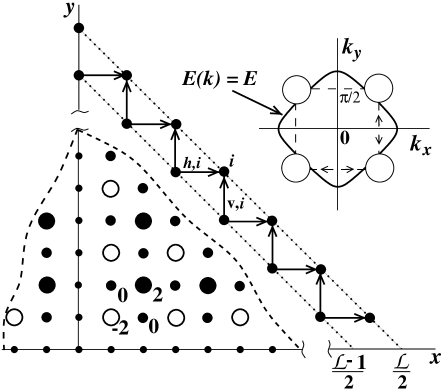
FIG. 1.: Shown is one quadrant of square with a side ${\cal L}/\sqrt{2}$. On-site energies in the presence of a period-doubling fluctuation are shown in the units of $V_{0}$; $\pi$-phase slip is shown only in the $x$-direction. Inset: solid line is a surface $E(\mathchoice{{\hbox{\boldmath$\displaystyle k$}}}{{\hbox{\boldmath$\textstyle k$}}}{{\hbox{\boldmath$\scriptstyle k$}}}{{\hbox{\boldmath$\scriptscriptstyle k$}}})=E$. Dotted lines are regions in $\textstyle k$-space perturbed by the fluctuation.

FIG. 2.: (a) Numerical coefficient $C_{E}$ in the dependence $|\ln f_{2}(E,t)|=C_{E}\ln^{2}(t/{\cal T}_{2})$ is plotted from Eq. (13) versus the disorder strength, $W$, at different energies. Dotted line is a weak-disorder asymptotics, $C_{E}\propto W^{-2}$. Inset: $C_{E}(W)$ at $E=2$ is shown in the domain of the weak disorder. (b) Wave function of an ALS with a decrement $\gamma_{3}=0.7$ in a cube with a side $L=12$ is shown in lexicographic order $m\rightarrow L^{2}(m_{x}-1)+L(m_{y}-1)+m_{z}$.

REFERENCES

[1] B. L. Altshuler, V. E. Kravtsov, I. V. Lerner,
in Mesoscopic Phenomena in Solids, eds. B. L. Altshuler,
P. A. Lee, and R. A. Webb (North Holland, Amsterdam, 1991).
[2] B. A. Muzykantskii and D. E. Khmelnitskii,
Phys. Rev. B 51, 5480 (1995).
[3] V. I. Fal’ko and K. B. Efetov,
Phys. Rev. B 52, 17413 (1995).
[4] A. D. Mirlin, Phys. Rep. 326, 259 (2000).
[5] V. G. Karpov, Phys. Rev. B 48, 4325 (1993);
V. M. Apalkov, M. E. Raikh, and B. Shapiro,
Phys. Rev. Lett. 89, 126601 (2002).
[6]P. W. Anderson, Phys. Rev. 109, 1492 (1958).
[7]A. MacKinnon and B. Kramer,
Phys. Rev. Lett. 47, 1546 (1981).
[8] E. Abrahams, P. W. Anderson, D. C. Licciardello,
and T. V. Ramakrishnan, Phys. Rev. Lett. 42, 673 (1979) .
[9] K. Slevin and T. Ohtsuki, Phys. Rev. Lett.
82, 382 (1999).
[10] H. Grussbach and M. Schreiber,
Phys. Rev. B 51, 663 (1995), and references therein.
[11] B. Huckestein and L. Schweitzer,
Phys. Rev. Lett. 72, 713 (1994).
[12]I. Kh. Zharekeshev and B. Kramer,
Phys. Rev. Lett. 79, 717 (1997).
[13]M. L. Ndawana, R. A. Römer,
and M. Schreiber, Eur. Phys. J. B 27, 399 (2002), and
references therein.
[14]Y. Asada, K. Slevin, and T. Ohtsuki,
Phys. Rev. Lett. 89, 256601 (2002), and references therein.
[15] S. Hikami, A. I. Larkin, and
Y. Nagaoka, Prog. Theor. Phys. 63, 707 (1980).
[16]K. Slevin and T. Ohtsuki, Phys. Rev. Lett.
78, 4083 (1997), and references therein.
[17]P. Markoš, Phys. Rev. B 65, 104207 (2002),
and references therein.
[18]K. Slevin, P. Markoš, and T. Ohtsuki,
Phys. Rev. Lett. 86, 3594 (2001); Phys. Rev. B 67,
155106 (2003).
[19] V. Uski, B. Mehlig, R. A. Römer,
and M. Schreiber, Phys. Rev. B 62, R7699 (2000).
[20]V. Uski, B. Mehlig,
and M. Schreiber, Phys. Rev. B 63, 241101(R) (2001).
[21]V. Uski, B. Mehlig, and M. Schreiber,
Phys. Rev. B 66, 233104 (2002).
[22]B. K. Nikolić, Phys. Rev. B 64,
014203 (2001).
[23]B. K. Nikolić, Phys. Rev. B 65,
012201 (2002).
[24]B. K. Nikolić, V. Z. Cerovski,
Eur. Phys. J. B 30, 227 (2002).
[25] M. Patra, Phys. Rev. E 67, 065603(R) (2003).
[26] A. Ossipov, T. Kottos, and T. Geisel,
Phys. Rev. E 65, R055209 (2002).
[27] L. I. Deych, M. V. Erementchouk, A. A. Lisyansky,
and B. L. Altshuler, preprint cond-mat/0304440.
[28]R. E. Peierls, Quantum Theory of Solids
(Clarendon, Oxford, 1955), p. 108.
[29] W. P. Su, J. R. Schrieffer, and A. J. Heeger,
Phys. Rev. Lett. 42, 1698 (1979).